Abstract
The invasive morning glory, Ipomoea purpurea (Convolvulaceae), poses a mounting challenge in vineyards by hindering grape harvest and as a secondary host of disease pathogens, necessitating advanced detection and control strategies. This study introduces a novel automated image analysis framework using aerial images obtained from a small fixed-wing unmanned aircraft system (UAS) and an RGB camera for the large-scale detection of I. purpurea flowers. This study aimed to assess the sampling fidelity of aerial detection in comparison with the actual infestation measured by ground validation surveys. The UAS was systematically operated over 16 vineyard plots infested with I. purpurea and another 16 plots without I. purpurea infestation. We used a semi-supervised segmentation model incorporating a Gaussian Mixture Model (GMM) with the Expectation-Maximization algorithm to detect and count I. purpurea flowers. The flower detectability of the GMM was compared with that of conventional K-means methods. The results of this study showed that the GMM detected the presence of I. purpurea flowers in all 16 infested plots with 0% for both type I and type II errors, while the K-means method had 0% and 6.3% for type I and type II errors, respectively. The GMM and K-means methods detected 76% and 65% of the flowers, respectively. These results underscore the effectiveness of the GMM-based segmentation model in accurately detecting and quantifying I. purpurea flowers compared with a conventional approach. This study demonstrated the efficiency of a fixed-wing UAS coupled with automated image analysis for I. purpurea flower detection in vineyards, achieving success without relying on data-driven deep-learning models.
1. Introduction
Tall morning glory Ipomoea purpurea (L.) Roth is an annual climbing vine and a troublesome weed in many annual and perennial crop fields. With over 500 species, Ipomoea is the largest genus in the family Convolvulaceae [1,2]. While some species within the genus are considered invasive weeds, not all species exhibit invasive behavior. I. purpurea is a highly sought-after ornamental plant that graces many cultivated gardens. They feature vibrant, purple-hued, trumpet-shaped blossoms, and their rapid growth and climbing nature underscore their aesthetic allure. I. purpurea has distinctive, heart-shaped, alternating leaves with inflorescences consisting of axillary clusters that are either solitary to a few or in groups of three to five. The flowers are funnel form with purple corollas (2–6 mm in length), which can possess a blue to white hue with a white center [3]. I. purpurea can produce 5000–26,000 seeds per plant [4], and thus, it is vital to apply control methods before the production and distribution of seeds to prevent the spread of this weed. While pre-planting, pre-emergence, and post-emergence applications of herbicides are commonly used to control I. purpurea in agronomic crops, it still can be difficult to control with herbicides when both the weed and crop share physiological similarities or when both exhibit vining growth and become entangled, compromising select control measures [4,5]. If I. purpurea is not controlled, it can reduce yield by 25% to 90% in various crops [4].
To manage I. purpurea in vineyards, a weed cutter or weed knife is commonly used to reduce the weed population in the orchard [6]. Although the shading effect of plants can keep I. purpurea under control in general, the weed becomes a greater nuisance in vineyards due to the lack of shade and the difficulty in the use of the weed knife [6]. Although growers can also apply salt, kerosene, lime, and other substances to control I. purpurea in vineyards, the applications must be spread all over the infested area because of the habits of the roots and rootstocks, which makes the cost so high that these materials can be used profitably in only a limited number of cases [6]. I. purpurea is sometimes found growing in patches, but it is more common to find patches distributed throughout a field [6]. I. purpurea has become an increasingly problematic species because of the increased use of glyphosate [7,8]. In addition to the weedy nature of I. purpurea, Wistrom and Purcell [9] detected Xylella fastidiosa, a causative bacterial agent of Pierce’s disease of grapevine, in I. purpurea. Therefore, the need for weed control in and near vineyards has become more important, especially in regions with chronic Pierce’s disease and established populations of sharpshooters, a major insect vector of the disease. Various chemical and cultural weed control methods have been developed [6,10], but they still can be problematic when the detection of I. purpurea is needed in large areas.
Pest detection over large areas can assist in understanding the ecology or epidemiology of pests such as insects, plant diseases, and weeds [11]. When the pattern of pest distribution is described with accurate detection methods, logical hypotheses about factors driving the distribution can be explored and used to develop new pest management strategies [12] including site-specific or spatially targeted pest management. While remote sensing to acquire aerial imagery by using manned aircraft is well established, it carries with it an inherent risk of crashes and loss of life and property. Therefore, the current unmanned aircraft system (UAS) technology has become an attractive tool for safe aerial surveys of crop stress and pests such as weeds. The UAS can be classified into fixed-wing and rotary-wing UASs. Each type of UAS has its advantages and drawbacks in the context of applications in agriculture. A rotary-wing UAS does not need forward motion to stay aloft, and instead leverages the vertical thrust generated by the propulsion system. It can hover and fly very slowly, which provides the potential for acquiring high-resolution aerial imagery. However, the major disadvantages of a rotary-wing UAS are its limited range and flight duration, mainly due to the capacity of the onboard battery. In contrast to a rotary-wing UAS, a fixed-wing UAS leverages the forward thrust generated by an engine to stay aloft. This has the advantage of long endurance flights, which are desirable when it comes to surveying large areas. However, a disadvantage of a fixed-wing UAS for this application is its need for a clear runway for takeoffs and landings and its inability to precisely hover at a location. Therefore, using a fixed-wing UAS for detecting weeds is recommended at landscape scales [13].
Previous studies presented a small UAS as a promising tool in agriculture [13,14,15,16,17,18,19], although the studies generally concentrated on mechanical configurations of the UAS [20,21]. For aerial detection of weed species, most of the previous studies utilized rotary-wing UASs. These studies include Rasmussen et al. [22], who used a rotary-wing UAS to test practical applications of UAS imagery and reported that one image at a 50 m altitude covered a 0.2 ha area without losing information about the cultivation impacts on vegetation. Torres-Sanchez et al. [23] also used a rotary-wing UAS to capture aerial images for early season weed management by using the image spatial and spectral properties required for weed seedling discrimination. Hameed and Amin [24] detected weeds in a wheat field by using image segmentation and classification based on images acquired with a rotary-wing UAS. The UAS also has been used for site-specific weed management. Example studies include the use of two separate UASs for weed mapping and site-specific spraying in sod fields [25] and the development of a computer vision algorithm for mapping the spatial distribution of weeds and creating a prescription map to perform site-specific weed control in a cornfield [26]. Shahi et al. [27] developed deep learning-based segmentation models for weed detection using an RGB image dataset acquired with a UAS. All of these studies indicated that a small rotary-wing UAS could be a potential tool for site-specific weed management. However, when a large landscape is the subject of the aerial survey, a fixed-wing UAS is more suitable as a main platform because it can cover large areas in a short period [13].
This study introduces a novel automated image analysis framework using aerial images obtained with a small fixed-wing UAS for the large-scale detection of I. purpurea flowers in vineyards. The objective of this study was to develop an automated image analysis protocol and determine the sampling fidelity of the aerial detection of I. purpurea flowers to actual infestation measured by ground survey. In addition, this study tested a fixed-wing UAS as part of a search for an inexpensive, user-friendly, and reliable aircraft for practical applications of a UAS for the large-scale aerial detection of I. purpurea infestation in vineyards. The new methods developed in this study will enhance the identification and detection of I. purpurea and contribute to species-specific and site-specific weed management in horticultural and perennial crops.
2. Materials and Methods
2.1. Study Site and Ground Truthing
This study was conducted in a vineyard located near Arvin, CA, USA (Figure 1a). The vineyard was planted with the grape (Vitis vinifera) variety Flame and suffered from I. purpurea infestation (Figure 1b). A total of 32 plots were established within the vineyard: 16 plots infested with I. purpurea and 16 plots without infestation. The size of each plot was 3 m by 6 m, which included two grapevines in the same row. The geocoordinates of each grapevine were recorded with a handheld GPS with <1 m resolution (GeoXT, Trimble, Sunnyvale, CA, USA). The UAS was flown over the 32 plots at two altitudes: 44 ± 2.5 m and 96 ± 8.2 m above the vineyard to capture aerial images.
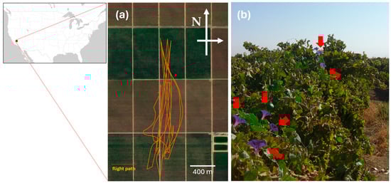
Figure 1.
Study site in a vineyard located in Arvin, CA, USA. The area of vineyard blocks surveyed for this study was ca. 65.5 ha (1560 m by 420 m). (a) GPS ground track of the UAS flight and (b) a ground view of I. purpurea infestation. The red dot on the map indicates the location of the study site, orange lines in (a) indicate the flight path of the UAS, and red arrows in (b) indicate I. purpurea flowers.
2.2. Unmanned Aircraft System (UAS) and Imaging System
A remotely controlled fixed-wing UAS (a.k.a., Foamy) was used to capture aerial images (Figure 2). The UAS is typically used as a disposable one; however, for this study, it was modified to include a rudder for directional control and an internal structure to house the imaging payload and the onboard flight data acquisition system (Table 1).
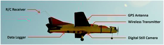
Figure 2.
The fixed-wing UAS model (MiG-27 Foamy) used in this study. Please see Table 1 for detailed specifications of the UAS.

Table 1.
Specifications of the UAS model (MiG-27 Foamy) used in the study.
A digital camera, Canon EOS Rebel XTi (Canon Inc., Tokyo, Japan), was used as the onboard imaging device. A small subset of its specifications is listed in Table 2. The camera captured digital images in continuous and remote trigger mode. Additionally, the camera was equipped with a standard EF-S 18–55 mm lens. To trigger the image capture from the ground, the onboard camera was interfaced with a remote trigger (Remote Switch RS-60E3, Canon Inc., Tokyo, Japan). The remote trigger was mechanically activated by the ground pilot using a mechanical servo connected to one of the RC channels. When a two-position switch on the transmitter was toggled, an arm attached to the servo activated the remote switch, which then activated the camera shutter. The camera was set up in a continuous burst mode, which captured up to 27 frames of images per activation.
Table 2.
Onboard imaging payload specifications.
The UAS was integrated with an onboard data acquisition system (Eagle Tree Seagull Wireless Data Acquisition, Eagle Tree Systems LLC, Bellevue, WA, USA). The data acquisition system recorded the GPS flight path of the UAS, as well as the inputs from the remote-control (RC) receiver (i.e., flight time stamps, flight altitude, flight speed, flight path, and camera shutter trigger) at a user-selected frequency. During the field operation of the UAS, the data rate was set at 10 Hz. Once aerial images were downloaded from the UAS, a composite image was generated using the software Pix4Dmapper (Pix4D, Prilly, Switzerland, https://www.pix4d.com/product/pix4dmapper-photogrammetry-software/, accessed on 11 February 2024) and Photoshop CS4 (Adobe Inc., San Jose, CA, USA). The composite image was georeferenced to confer spatial attributes to the map coordinate system, i.e., ortho-mosaicking with ArcInfo® 10 (ESRI, Redland, CA, USA). Both individual and composite images were used for the detection of I. purpurea flowers in this study.
2.3. Machine Learning
Aerial images were cropped into the 32 plots (16 plots with I. purpurea and 16 plots without I. purpurea) to extract information about I. purpurea flowers. One of the 16 images with I. purpurea served as the representative image to teach the features to the model. The framework was organized into three segments: the Image-Driven Feature Extraction Block (supervised block), the Gaussian Mixture Model (GMM; unsupervised block), and the flower counter (Figure 3).
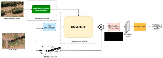
Figure 3.
Overall enhanced Gaussian Mixture Model (GMM) framework for the detection and counting of I. purpurea flowers on aerial images with unsupervised and supervised modules.
2.3.1. Image-Driven Feature Extraction Block
The representative image was initially converted into a grayscale image to eliminate the shadows from the grapevine rows. The average intensity of the grayscale image was evaluated, and a binary mask with a threshold of 0.7 was applied to remove shadows. This threshold was adjusted based on lighting conditions. The thresholded mask was then applied to the original representative image, separating the regions of interest (RoIs), i.e., the vineyard blocks from the shadow regions. The segmented image was then converted into an HSV (hue, saturation, and value) color space to accurately identify the purple I. purpurea flowers [28]. Such shadow removal was crucial for this framework to avoid false positives in the shadow regions during segmentation. Following the HSV transformation, we selected two I. purpurea flower regions within the segmented HSV image. As the RoIs were selected only from one image to train our GMM (i.e., the unsupervised block), we used data augmentation [29] to provide information about the various lighting conditions and camera angles. Each manually selected RoI was subjected to three different data augmentations (i.e., cropping, scaling, and brightness adjuster), thereby creating four new RoIs (one original and three augmented) to train the unsupervised block. We used two manually selected RoIs in this work, yielding eight RoI images. These images were converted into a 2-D array containing the flower pixel values. This entire block was the supervised aspect in our framework as this 2-D array with flower pixel values was used to teach the color distribution of I. purpurea flowers to the GMM. The overall architecture of the Image-Driven Feature Extraction Block is shown in Figure 4, and a single NVIDIA GeForce RTX 3090 GPU was used for machine learning.

Figure 4.
Overview of the Image-Driven Feature Extraction Block (supervised module).
2.3.2. Gaussian Mixture Model (GMM) Initialization
The RGB image of a plot containing I. purpurea flowers was transformed into an HSV color space to separate color (hue and saturation) from brightness (value). This separation was necessary when dealing with varying lighting conditions, as it decoupled color variations from changes in brightness, enhancing the accuracy and adaptability of segmentation and thereby providing a more robust segmentation model. The HSV image was then fed to the GMM block for predicting the presence of I. purpurea flowers. The GMM was trained using the information from flower pixels learned in the Image-Driven Feature Extraction Block (Figure 3). The trained GMM was then applied to the HSV image to determine which pixels in the image were likely to belong to I. purpurea flower regions. This prediction was based on how closely the color of each pixel in the image matched the color distribution learned from flower pixels.
The GMM is a statistical framework that characterizes the image’s underlying distribution of pixel values using the Expectation-Maximization (EM) algorithm [30]. The GMM comprises Gaussian components, each representing a potential cluster of pixel values in the image. In our study, the critical parameters of the GMM were the mean vector (µ), covariance matrix (Σ), and mixing coefficient (π). The mean vector comprised one value for each channel (H, S, and V). These values were used to obtain the average H, S, and V values of the pixels potentially belonging to a particular cluster. The covariance matrix captured the spread and interdependencies among the H, S, and V values within the cluster, signifying how the pixel values within the cluster vary relative to each other. Finally, the mixing coefficient represented the weight or proportion of the cluster in the overall mixture. It determined the significance of the cluster in modeling the pixel distribution, thereby giving the prior probability. We initialized the model and then used the EM algorithm to refine the parameters. The mean values of the Gaussian components were initialized using K-means clustering to select initial means for the Gaussian components. These means were positioned based on cluster centers in the data. The covariance matrices were initialized as spherical covariance matrices, where each covariance matrix was initialized with the same scalar value computed as the average of the variances in the data dimensions. This initialization assumed independence between dimensions. Finally, the mixing coefficients were initialized with equal weights, considering that each Gaussian component was assumed to be equally likely at the beginning of the EM algorithm’s iterations. During the EM process, these coefficients were adjusted to reflect the actual data distribution. The GMM was initialized by setting the number of Gaussian components/clusters to K (K = 2 in our study).
The Expectation-Maximization (EM) Algorithm
We used a 2-step EM algorithm, an iterative optimization technique, to estimate the parameters of the GMM. In the expectation step (E-step), we evaluated the probability of each pixel’s membership in each Gaussian component. This probability provided us with the likelihood of a pixel’s H, S, and V values belonging to a specific Gaussian component. The calculation used the Gaussian Probability Density Function (PDF) [31], which characterized the probability distribution of pixel values. The following equation (Equation (1)) was used for the Gaussian PDF:
where x represents the vector of H, S, and V values of the pixel under consideration, µk is the mean vector for the Gaussian component (cluster) k containing the average H, S, and V values for the pixels that may belong to this cluster, and Σk is the covariance matrix for the Gaussian component k that captures the spread and relationships between the H, S, and V values within the cluster.
Within the E-step, we evaluated the probability of each pixel’s membership in each Gaussian component, determining their respective responsibilities (posterior probabilities). These posterior probabilities represented the likelihood that a pixel belonged to each Gaussian component, and they played a vital role in the subsequent steps of the algorithm. Mathematically, the posterior probability P(zik = 1|xi) for data point xi and component k represents the probability that data point xi belongs to component k, given the observed data point xi and the current model parameters. For each pixel in the image, we calculated the posterior probabilities (responsibilities) of belonging to each Gaussian component (k) using the following formula (Equation (2)):
where xi is the vector of H, S, and V values of the ith pixel, f (xi | µk, Σk) is the likelihood of a single Gaussian component calculated using the Gaussian PDF (Equation (1)), πk is the mixing coefficient that gives the prior probability for component k, and zik represents the cluster assignment of data point xi to cluster k. The latent variable zik is binary and takes on one of two values (i.e., 1 or 0). When zik is equal to 1, it indicates that data point xi belongs to cluster k, and when it is equal to 0, it suggests that data point xi does not belong to cluster k. This E-step operation iterated over all pixels in the image, effectively assessing their associations with the Gaussian components. In essence, the Gaussian PDF quantified how well a pixel’s color and intensity align with the characteristics of a given cluster. Smaller distances between the pixel’s values (x) and the mean (µ), adjusted by the covariance (Σ), indicate higher likelihoods. The resulting γ(zik) values provided the algorithm with a probabilistic understanding of the pixel–cluster relationships, serving as a critical foundation for the subsequent maximization (M-step), where the Gaussian component parameters (µ, Σ, and π) were updated to optimize the model.
In the maximization step (M-step), the parameters of the Gaussian components (mean vectors, covariance matrices, and mixing coefficients) were updated to maximize the likelihood of the observed data based on the posterior probabilities computed in the E-step. The updated mean vector for each component (cluster) k provided a new mean vector () for component k calculated as the weighted average of all data points xi, where the weights were the posterior probabilities P(zik = 1|xi), indicating the likelihood that data point xi belonged to component k, which is given by (Equation (3)).
where N is the total number of data points. The new mean vector reflected a weighted average of the data points, with each data point’s weight determined by its likelihood of belonging to component k. Similarly, the covariance matrices for each component k were updated by computing the new covariance matrix (Equation (4)). The new covariance matrix () for component k was calculated as the weighted summation of the outer products of the differences between data points (xi) and the new mean vector () with the weights being the posterior probabilities P(zik = 1|xi).
The weighted sum of the outer products generated more weight to data points that were more likely to belong to component k, thereby representing how the data points were spread out within the component. Finally, the mixing coefficients (Equation (5)) were updated, depicting the proportions of data points assigned to each component. The new mixing coefficient () for component k was calculated as the average of the posterior probabilities for all data points assigned to the component, and was used to normalize the sum, ensuring that the mixing coefficients summed up to 1, representing proportions.
After updating the parameters in the M-step, the EM algorithm proceeded to the E-step again. This iterative process continued until the convergence criteria were met, typically when the changes in parameters became small or when the log-likelihood of the data stabilized. The convergence of the EM algorithm relies on three key elements: the maximum number of iterations, log-likelihood change and tolerance, and parameter change. Firstly, to avert indefinite execution, a predefined maximum number of iterations was set to 100 to ensure computational efficiency and prevent the algorithm from running excessively. Secondly, the EM algorithm continuously monitored the change in the log-likelihood of the observed data between consecutive iterations. A tolerance level, usually set to e−3, acted as a convergence threshold. When the change in log-likelihood dropped below this threshold, further iterations did not yield substantial improvements. Consequently, the algorithm concluded that the model had converged. Finally, the algorithm assessed changes in the GMM’s parameters, encompassing means, covariances, and mixing coefficients. Convergence was indicated when these parameter changes became smaller than the specified tolerance. This change reflected the stabilization of model parameters, culminating in convergence.
2.3.3. Gaussian Clustering and Segmentation
To predict the segmentation labels for each pixel in the original HSV image, we determined which Gaussian component (cluster) a pixel was most likely to belong to given its color and brightness attributes. To achieve this, we calculated the probability of a pixel belonging to each cluster using the Gaussian PDF (Equation (1)), which measured how well a pixel’s color aligns with the characteristics of a particular cluster. Each pixel was assigned to the cluster with the highest probability, resulting in segmentation labels for the entire image. These labels partitioned the image into regions, with each region potentially representing a different object or area of interest based on color and intensity characteristics. Thus, the preliminary boundaries that separated the I. purpurea flowers from the background within the HSV image were created.
The segmentation labels produced were initially organized in a format that matched the flattened image. When this format did not align with the spatial layout of the original image, we reshaped the labels to match the spatial arrangement of the original image. This transformation ensured that each pixel’s assigned cluster corresponded to its correct location in the image. The result was a label map that mirrors the image’s dimensions, allowing us to understand where each segment was located within the image.
A binary map was generated to distinguish the segmented regions clearly. In this map, each pixel was assigned a binary value, usually 1 or 0, indicating whether the pixel belonged to a particular cluster or not. We chose one of the clusters, often the one representing I. purpurea flowers, and assigned it a binary value of 1, while the other clusters (background) received a value of 0. This binary map outlined the segmented regions within the image, making it easier to visualize and analyze the results. These binary flower map pixel values were normalized to the 0–255 range to ensure these maps could be processed, displayed, and analyzed consistently and effectively. The overall workflow is shown in Figure 5.
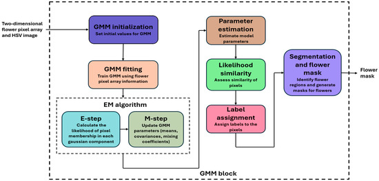
Figure 5.
Gaussian Mixture Model (GMM; unsupervised module) architecture with inputs as the 2-D flower pixel array from the supervised module and the HSV image and output as a binary flower mask indicating the presence of I. purpurea.
2.3.4. Counting I. purpurea Flowers
The flower size was used to count the I. purpurea flowers in the aerial images. As the number of pixels per flower could vary with different drone flight altitudes, we tailored the minimum and maximum pixel count thresholds to each distinct flight altitude level, thus addressing the inherent variability in flower sizes that often correlated with flight altitude. The binary flower mask was loaded with white pixels as I. purpurea flowers and the rest as background (black pixels). Depending on the flight altitude, we manually selected the minimum and maximum pixel count thresholds. These thresholds determined the range of pixel counts considered as a single flower. Any connected region with a pixel count falling within this range was counted as a single flower. The connected components in the binary flower mask were identified, and a unique label was assigned to each connected region and provided statistics for each component, including its area (pixel count) and centroid. The flower counter was then initialized to keep track of the total number of flowers in the image. We checked each labeled component’s pixel count against the defined thresholds (minimum and maximum pixel thresholds). If the pixel count of a component fell within the threshold range, it was directly counted as a single flower. If the pixel count was above the threshold, an average size between the minimum and maximum pixel count thresholds was calculated to estimate the number of flowers in that region. After processing all connected components, the total count of flowers in the image was given. This approach ensures that both small and large clusters of flowers are accurately quantified. An overview of the algorithm is given below (Algorithm 1).
| Algorithm 1: I. purpurea Flower Counter |
| Input: Segmented binary flower mask of the high-altitude UAS image. Output: Total number of I. purpurea flowers in the image. Step 1: Initialize Total_Flower_Count = 0; Step 2: Load the flower mask of the high-altitude UAS image; Step 3: Prompt the user to select altitude; Step 4: Determine minimum and maximum pixel count thresholds based on altitude; Step 5: Apply Connected Component Analysis on the binary flower mask; Step 6: for Each connected component in the mask do 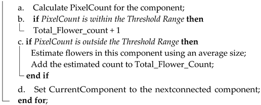 Step 7: Return Total_Flower_Count as the total number of I. purpurea flowers in the image; Step 8: End. |
2.4. Evaluation of the Gaussian Mixture Model (GMM)
We used various error metrics to evaluate and quantify the performance of both our enhanced GMM and the conventional K-means algorithm. In this study, we leveraged Root Mean Square Error (RMSE), Mean Absolute Error (MAE), and Max error to compare the models’ accuracy. RMSE (Equation (6)) serves as a robust precision measurement emphasizing the importance of accurate predictions by considering the average magnitude of differences between the predicted (Xpred) and the ground-truth values (Xtrue), thereby optimizing the predictive accuracy. On the other hand, MAE (Equation (7)) provides a measure of overall accuracy by determining the average absolute differences between predictive (Xpred) and the ground-truth values (Xtrue). Lastly, Max error (Equation (8)) identifies the maximum deviation between the predicted and ground-truth values, which was crucial for pinpointing the potential outliners.
To assess the predictive models in the specific task of I. purpurea flower counting, we used three key bias metrics: the Bias Ratio (BR), the Scaled Mean Bias Residual (SMBR), and the Fractional Bias (FB). These metrics provide a comprehensive evaluation of the models’ performance. The BR measures the average deviation between the predicted (Xpred) and true counts (Xtrue) relative to the true counts, with lower values indicating greater accuracy (Equation (9)). A negative BR indicates an underestimation, indicating that the predictive counts are lower than the true counts. Conversely, a positive BR indicates an overestimation.
The MBR (Equation (10)) calculates the average difference between the predicted and the true counts. The SMBR scales the MBR to a standardized range of −1 to 1, facilitating fair assessments and model comparisons regardless of the inherent scales or characteristics of the predictions. The Scaled Mean Bias Residual (SMBR) is a normalized indicator of bias, which underscores the efficacy of the GMM by scaling the Mean Bias Residual (MBR) to a standardized range of −1 to 1 (Equation (11)).
Finally, the Fractional Bias (FB) captures the proportional differences between the predicted and true counts (Equation (12)), affirming the superiority of the GMM in proportional prediction precision.
3. Results
The semi-supervised segmentation with an enhanced GMM framework we developed in this study successfully identified I. purpurea flowers in aerial images and was also able to count the number of flowers (Figure 6).
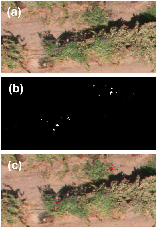
Figure 6.
Illustration of our enhanced GMM framework application to an RGB image depicting: (a) the input: original RGB image, (b) the predicted binary mask: output of our enhanced GMM highlighting I. purpurea flower regions, and (c) the segmented output: application of the binary mask to the original RGB image, emphasizing the identified flower locations and providing a total count estimate. White dots in (b) and red dots in (c) indicate I. purpurea flowers detected by the enhanced GMM.
From the ground survey of 16 plots infested with I. purpurea, we found that the average number of I. purpurea flowers was 39.1 ± 31.25 per grapevine (Table 3). The number of I. purpurea flowers detected by the GMM and K-means methods were 29.8 ± 22.54 and 25.6 ± 19.61 per grapevine, respectively. This result indicates that the GMM method detected more flowers on the aerial images than the K-means method.
Table 3.
Comparative flower count predictions between conventional K-means and enhanced GMM methods.
In our comparative analysis, our enhanced GMM consistently outperformed the conventional K-means method across all the metrics (i.e., lower RMSE, MAE, and Max error values), indicating the reliability of our model in accurately counting I. purpurea flowers (Table 4).
Table 4.
Error metrics comparison between K-means clustering and our enhanced GMM with Root Mean Square Error (RMSE), Mean Absolute Error (MAE), and Max error.
The results of our study showed that the K-means predictions diverge from the actual I. purpurea flower count, indicating potential challenges in capturing spatial distribution patterns (Figure 7a). In contrast, our enhanced GMM exhibited more consistent alignment with the ground-truth values, indicating an accurate capture of I. purpurea distribution. Our results show that K-means consistently underestimated the flower count, while our model maintained a closer alignment with the true values across all the altitudes. The K-means predictions tended to fluctuate more widely than our GMM predictions, indicating a less accurate count across various instances of I. purpurea flowers.
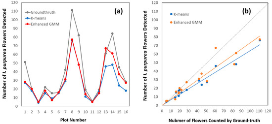
Figure 7.
Comparison between the conventional K-means and our enhanced GMM methods for detecting I. purpurea flowers using a line plot (a) and regression (b). The dotted line in (b) indicates a perfect match between ground and aerial survey results (i.e., y = x).
The regression analyses showed that the GMM (slope = 1.309; d.f. = 1, 14; F = 116.0; R2 = 0.89) and K-means (slope = 1.558; d.f. = 1, 14; F = 311.9; R2 = 0.96) methods detected 76% and 65% of the flowers, respectively (Figure 7b).
The results of this study showed that the GMM detected the presence of I. purpurea flowers in all 16 infested plots with 0% for both type I and type II errors, while the K-means method had 0% and 6.3% for type I and type II errors, respectively. The GMM and K-means methods detected 76% and 65% of the flowers, respectively.
In addition, the BR, SMBR, and FB were used for a holistic assessment of our enhanced performance of the GMM in I. purpurea flower counting from aerial imagery. The GMM demonstrated a BR value of −0.239, outperforming that of K-means (−0.345) and indicating better alignment with the actual number of I. purpurea flowers. The GMM exhibited an SMBR of −0.6944, indicating a more normalized and reduced bias, while K-means registered an SMBR of −1.0. The FB value from the GMM (−0.1986) surpassed that of K-means (−0.2989), affirming a higher accuracy was achieved by the GMM in predicting proportional variations.
The values of the BR, SMBR, and FB collectively offer insights into accuracy, bias normalization, and proportional prediction precision (Figure 8). Our results showed that both K-means and our enhanced GMM tend to underestimate the overall I. purpurea flower count, but the enhanced GMM performed better based on lower FB and more refined SMBR values, which aligned with a more conservative approach that is often favored in precision agriculture. This strategy minimizes the risk of resource misallocation and unnecessary interventions, making our model a more reliable choice.
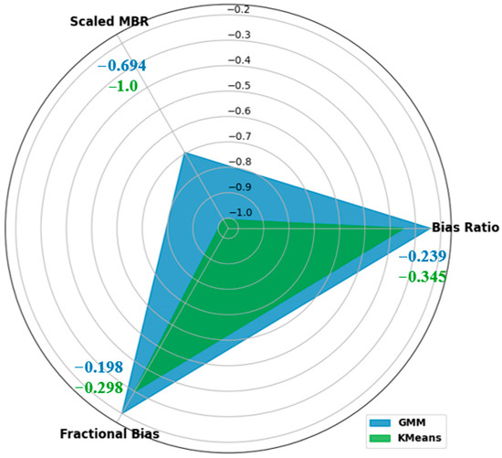
Figure 8.
Spider plot comparison of bias metrics (Bias Ratio, Scaled Mean Bias Residual, and Fractional Bias) between K-means and our enhanced GMM for I. purpurea flower detection and counting.
Overall, the results of our study showed that the enhanced GMM consistently outperformed conventional K-means. Our study also demonstrated that the detection and number of I. purpurea flowers using the enhanced GMM closely aligned with the ground-truth data, emphasizing the precision of our model in challenging visual conditions like low image resolution and offering a robust solution for the flower detection and counting problem.
4. Discussion
Traditionally, precision weed management utilizes optical sensors mounted on ground vehicles [32]. However, the ground sensing of weeds becomes very challenging at a large scale and in very dense weed populations. With recent advances in UAS and sensor technologies, aerial surveys have become a key method for precision agriculture and smart farming because UASs can cover a larger area of land in less time for the creation of weed and treatment maps. In addition, the UAS has found widespread applications in crop and soil monitoring [33,34,35], pest detection [22,36,37], aerial release of natural enemies [38,39], and pesticide application [40]. In this study, we developed an automated method for detecting I. purpurea flowers using an enhanced GMM. Because I. purpurea can be readily removed by the use of a weed knife [6] rather than applying herbicide throughout the vineyard, locating individual patches of I. purpurea flowers can guide where to visit and control the weed mechanically and site-specifically. We opted for a fixed-wing UAS as a near-real-time and cost-effective aerial survey tool in this study. While it cannot hover or hold a position over a specific location for detailed remote sensing, its extended flight endurance and longer duration, compared with a rotary-wing UAS, offer the potential for large-scale pest detection and site-specific weed management. Moreover, the flexibility of the UAS and the modularity of its onboard payload allow for easy retrofits with a variety of high-resolution imaging payloads. The implementation of an onboard control system enables tailored UAS flights to meet site-specific monitoring strategies, with the ability to program coverage of specific areas requiring additional monitoring. Recent significant advances in miniaturized flight control technology, coupled with the expanded capabilities of the UAS for autonomous flight, open the possibility of conducting these aerial surveys repeatedly and potentially even without human intervention.
In this study, we found that I. purpurea flowers were too small to be characterized by the existing region-based object detection methods; I. purpurea flowers in the image formed clusters of 5–10 pixels, suggesting that the color of the flower is a more reliable feature than shape or region for this specific application. Therefore, we compared the performance of semi-supervised machine learning algorithms, K-means, and our enhanced GMM for the detection and estimation of I. purpurea flowers in aerial images. Our enhanced GMM approach provided a comprehensive solution by combining the strengths of unsupervised and supervised learning, addressing specific challenges and enhancing the robustness of I. purpurea flower detection in aerial images compared with traditional GMM and K-means methods. In contrast to traditional GMM, our model incorporated user interaction, allowing for manual selection of I. purpurea regions and providing a semi-supervised aspect. This not only refined the GMM by utilizing specific RoIs for training but also introduced data augmentation to account for varying lighting conditions and camera angles, resulting in a more robust model. Our enhanced GMM outperformed K-means in I. purpurea flower detection due to its probabilistic nature and ability to model clusters of varying shapes and sizes. The probabilistic framework allowed the GMM to assign probabilities to data points, accommodating diverse flower characteristics. However, our model was computationally intensive and sensitive to component selection. K-means, on the other hand, while computationally efficient, fell short in capturing the granular distribution of I. purpurea flowers with its assumption of spherical clusters. Its simplicity and interpretability are advantages, but the rigid cluster shape assumption limits its applicability. The amalgamation of preprocessing, user-defined input, and data augmentation contributes to superior performance, making our approach a comprehensive and effective solution for I. purpurea flower detection in aerial imagery.
Our innovative approach to I. purpurea flower detection in aerial images diverges from data-driven deep learning models [41,42,43,44], emphasizing a combination of traditional image processing techniques and machine learning. Notably, our method distinguishes itself from conventional flower count clustering algorithms [41,45,46] by introducing a semi-supervised aspect. The semi-supervised nature of our approach significantly reduces reliance on large, annotated datasets, making it particularly advantageous in scenarios where obtaining extensive labeled data is challenging. This characteristic enhances the model’s adaptability and practicality, positioning it as a valuable solution for flower detection in aerial images while minimizing the need for extensive annotated datasets. By incorporating user interaction and semi-supervised learning into our enhanced GMM framework, we aim to generate accurate ground truths for future deep learning models [47,48]. Apart from I. purpurea flower counting, our method also provides valuable segmentation results (Figure 6). These segmentation results enable one to precisely identify the location of I. purpurea flowers by providing the spatial distribution. These insights aid in targeted interventions allowing for more efficient and resource-effective agricultural practices, contributing to improved yield and crop management. However, our model has some limitations. Uncertainties regarding adaptability may result in variable performance across real-world scenarios due to a lack of validation across diverse datasets and environmental conditions. Additionally, the subjectivity and reliance on manual input pose challenges for large-scale applications and efficiency. With the requirement of human effort for annotation in datasets with a high volume of images as well as difficulties with handling changes in lighting and camera angles, we may have scalability concerns. An alternative approach to automatic image analysis is learning-based methods, such as support vector machines (SVMs) [49] or the more recently developed convolutional neural networks (CNNs) [50]. In contrast to model-based methods like K-means and GMM clustering, learning-based methods rely on extensive training data to optimize a model for a specific analysis task. Therefore, the application of artificial intelligence and machine learning could further enhance automated image processing and weed detection capabilities in the future. We recognize the potential of few-shot learning [51] and zero-shot learning [52] in expanding the model’s capabilities, enabling it to adapt to new classes or variations in I. purpurea.
5. Conclusions
This study demonstrated that a combination of a fixed-wing UAS and automated image analysis could be used to effectively detect I. purpurea flowers in vineyards. In addition, the results of this study imply three important applications of the fixed-wing UAS along with automated image analysis for site-specific I. purpurea management in vineyards. Firstly, a low-cost fixed-wing UAS with an off-the-shelf camera can be used for a large-scale aerial survey of I. purpurea in vineyards. This overcomes the limitations of rotary-wing UASs including less flight endurance and shorter flight duration. Secondly, automated image analysis for detecting and counting I. purpurea flowers could be performed with semi-supervised segmentation with a GMM. Determining the location and number of I. purpurea flowers in vineyards is the key step for management decision-making and site-specific removal of I. purpurea by using control measures. Lastly, this system can be applied to places where a large-scale weed survey using a UAS is needed such as rangelands and open forests.
Author Contributions
Conceptualization, Y.-L.P., S.G. and X.L.; methodology, S.K.V., X.L., J.W., Y.-L.P. and S.G.; software, S.K.V. and J.W.; validation, Y.-L.P. and S.G.; formal analysis, J.W. and S.K.V.; investigation, S.K.V., X.L., J.W., Y.-L.P. and S.G.; resources, Y.-L.P.; data curation, S.K.V. and Y.-L.P.; writing—original draft preparation, S.K.V. and Y.-L.P.; writing—review and editing, X.L. and R.K.; visualization, S.K.V. and Y.-L.P.; supervision, Y.-L.P. and X.L.; project administration, Y.-L.P.; funding acquisition, Y.-L.P. All authors have read and agreed to the published version of the manuscript.
Funding
This research was supported by the USDA NIFA AFRI Foundational and Applied Sciences Grant Program (2021-67014-33757) and the Hatch Project (WVA00724) of West Virginia University.
Data Availability Statement
Data are contained within the article.
Acknowledgments
The authors appreciate the team of research collaborators from the University of California, Riverside (T. M. Perring, S. Baek, J. J. Park, and J. E. Nay), and West Virginia University (H. Straight, J. Gross and J. B. White) for their help with the field study.
Conflicts of Interest
The authors declare no conflicts of interest.
References
- Bhullar, M.S.; Walia, U.; Singh, S.; Singh, M.; Jhala, A.J. Control of morningglories (Ipomoea spp.) in sugarcane (Saccharum spp.). Weed Technol. 2012, 26, 77–82. [Google Scholar] [CrossRef]
- Singh, M.; Ramirez, A.H.; Sharma, S.D.; Jhala, A.J. Factors affecting the germination of tall morningglory (Ipomoea purpurea). Weed Sci. 2012, 60, 64–68. [Google Scholar] [CrossRef]
- Bryson, C.T.; DeFelice, M.S. Weeds of the Midwestern United States and Central Canada; University of Georgia Press: Athens, GA, USA, 2010. [Google Scholar]
- Jones, E.A.; Contreras, D.J.; Everman, W.J. Ipomoea hederacea, Ipomoea lacunosa, and Ipomoea purpurea. In Biology and Management of Problematic Crop Weed Species; Elsevier: Amsterdam, The Netherlands, 2021; pp. 241–259. [Google Scholar]
- Price, A.J.; Williams, J.P.; Duzy, L.A.; McElroy, J.S.; Guertal, E.A.; Li, S. Effects of integrated polyethylene and cover crop mulch, conservation tillage, and herbicide application on weed control, yield, and economic returns in watermelon. Weed Technol. 2018, 32, 623–632. [Google Scholar] [CrossRef]
- Cox, H.R. The Eradication of Bindweed, or Wild Morning-Glory; U.S. Department of Agriculture: Washington, DC, USA, 1909.
- Culpepper, A.S. Glyphosate-induced weed shifts. Weed Technol. 2006, 20, 277–281. [Google Scholar] [CrossRef]
- Webster, T.M.; Nichols, R.L. Changes in the prevalence of weed species in the major agronomic crops of the Southern United States: 1994/1995 to 2008/2009. Weed Sci. 2012, 60, 145–157. [Google Scholar] [CrossRef]
- Wistrom, C.; Purcell, A. The fate of Xylella fastidiosa in vineyard weeds and other alternate hosts in California. Plant Dis. 2005, 89, 994–999. [Google Scholar] [CrossRef] [PubMed]
- Lider, L.; Leonard, O. Morning glory control in vineyards with two new soil-residual herbicides: Dichlobenil and chlorthiamid. Calif. Agric. 1968, 22, 8–10. [Google Scholar]
- Park, Y.-L.; Krell, R.K.; Carroll, M. Theory, technology, and practice of site-specific insect pest management. J. Asia-Pac. Entomol. 2007, 10, 89–101. [Google Scholar] [CrossRef]
- Park, Y.-L.; Krell, R.K. Generation of prescription maps for curative and preventative site-specific management of bean leaf beetles (Coleoptera: Chrysomelidae). J. Asia-Pac. Entomol. 2005, 8, 375–380. [Google Scholar] [CrossRef]
- Hung, C.; Xu, Z.; Sukkarieh, S. Feature learning based approach for weed classification using high resolution aerial images from a digital camera mounted on a UAV. Remote Sens. 2014, 6, 12037–12054. [Google Scholar] [CrossRef]
- Schmale Iii, D.G.; Dingus, B.R.; Reinholtz, C. Development and application of an autonomous unmanned aerial vehicle for precise aerobiological sampling above agricultural fields. J. Field Robot. 2008, 25, 133–147. [Google Scholar] [CrossRef]
- Zhang, C.; Kovacs, J.M. The application of small unmanned aerial systems for precision agriculture: A review. Precis. Agric. 2012, 13, 693–712. [Google Scholar] [CrossRef]
- Garcia-Ruiz, F.; Sankaran, S.; Maja, J.M.; Lee, W.S.; Rasmussen, J.; Ehsani, R. Comparison of two aerial imaging platform for identification of Huanglongbing-infected citrus trees. Comput. Electron. Agric. 2013, 91, 106–115. [Google Scholar] [CrossRef]
- Rajeena, P.F.; Ismail, W.N.; Ali, M.A. A metaheuristic harris hawks optimization algorithm for weed detection using drone images. Appl. Sci. 2023, 13, 7083. [Google Scholar]
- Stephen, S.; Kumar, V. Detection and analysis of weed impact on sugar beet crop using drone imagery. J. Indian Soc. Remote Sens. 2023, 51, 2577–2597. [Google Scholar] [CrossRef]
- Castellano, G.; De Marinis, P.; Vessio, G. Weed mapping in multispectral drone imagery using lightweight vision transformers. Neurocomputing 2023, 562, 126914. [Google Scholar] [CrossRef]
- Xiang, H.; Tian, L. Development of a low-cost agricultural remote sensing system based on an autonomous unmanned aerial vehicle (UAV). Biosyst. Eng. 2011, 108, 174–190. [Google Scholar] [CrossRef]
- Mahony, R.; Kumar, V.; Corke, P. Multirotor aerial vehicles: Modeling, estimation, and control of quadrotor. IEEE Robot. Autom. Mag. 2012, 19, 20–32. [Google Scholar] [CrossRef]
- Rasmussen, J.; Nielsen, J.; Garcia-Ruiz, F.; Christensen, S.; Streibig, J. Potential uses of small unmanned aircraft systems (UAS) in weed research. Weed Res. 2013, 53, 242–248. [Google Scholar] [CrossRef]
- Torres-Sánchez, J.; López-Granados, F.; De Castro, A.I.; Peña-Barragán, J.M. Configuration and specifications of an unmanned aerial vehicle (UAV) for early site specific weed management. PLoS ONE 2013, 8, e58210. [Google Scholar] [CrossRef]
- Hameed, S.; Amin, I. Detection of weed and wheat using image processing. In Proceedings of the 2018 IEEE 5th International Conference on Engineering Technologies and Applied Sciences (ICETAS), Bangkok, Thailand, 22–23 November 2018; pp. 1–5. [Google Scholar]
- Hunter III, J.E.; Gannon, T.W.; Richardson, R.J.; Yelverton, F.H.; Leon, R.G. Integration of remote-weed mapping and an autonomous spraying unmanned aerial vehicle for site-specific weed management. Pest Manag. Sci. 2020, 76, 1386–1392. [Google Scholar] [CrossRef]
- Sapkota, R.; Stenger, J.; Ostlie, M.; Flores, P. Site-specific weed management in corn using UAS imagery analysis and computer vision techniques. arXiv 2022, arXiv:2301.07519. [Google Scholar]
- Shahi, T.B.; Dahal, S.; Sitaula, C.; Neupane, A.; Guo, W. Deep Learning-Based Weed Detection Using UAV Images: A Comparative Study. Drones 2023, 7, 624. [Google Scholar] [CrossRef]
- Trivedi, V.K.; Shukla, P.K.; Dutta, P.K. K-mean and HSV model based segmentation of unhealthy plant leaves and classification using machine learning approach. In Proceedings of the 3rd IET International Smart Cities Symposium, 3SCS-2020, Manama, Bahrain, 21–23 September 2020. [Google Scholar]
- Alomar, K.; Aysel, H.I.; Cai, X. Data augmentation in classification and segmentation: A survey and new strategies. J. Imaging 2023, 9, 46. [Google Scholar] [CrossRef] [PubMed]
- Dempster, A.P.; Laird, N.M.; Rubin, D.B. Maximum likelihood from incomplete data via the EM algorithm. J. R. Stat. Soc. Ser. B 1977, 39, 1–22. [Google Scholar] [CrossRef]
- Leon-Garcia, A. Probability and Random Processes for Electrical Engineering; Pearson Education Inc.: Upper Saddle River, NJ, USA, 2008. [Google Scholar]
- Singh, V.; Rana, A.; Bishop, M.; Filippi, A.M.; Cope, D.; Rajan, N.; Bagavathiannan, M. Unmanned aircraft systems for precision weed detection and management: Prospects and challenges. Adv. Agron. 2020, 159, 93–134. [Google Scholar]
- Mulla, D.J. Twenty five years of remote sensing in precision agriculture: Key advances and remaining knowledge gaps. Biosyst. Eng. 2013, 114, 358–371. [Google Scholar] [CrossRef]
- González-Jorge, H.; Martínez-Sánchez, J.; Bueno, M.; Arias, P. Unmanned aerial systems for civil applications: A review. Drones 2017, 1, 2–19. [Google Scholar] [CrossRef]
- Daponte, P.; De Vito, L.; Glielmo, L.; Iannelli, L.; Liuzza, D.; Picariello, F.; Silano, G. A review on the use of drones for precision agriculture. IOP Conf. Ser. Earth Environ. Sci. 2019, 275, 012022. [Google Scholar] [CrossRef]
- Park, Y.L.; Naharki, K.; Karimzadeh, R.; Seo, B.Y.; Lee, G.S. Rapid assessment of insect pest outbreak using drones: A case study with Spodoptera exigua (Hübner) (Lepidoptera: Noctuidae) in soybean fields. Insects 2023, 14, 555. [Google Scholar] [CrossRef]
- Naharki, K.; Huebner, C.D.; Park, Y.L. The detection of tree of heaven (Ailanthus altissima) using drones and optical sensors: Implications for the management of invasive plants and insects. Drones 2024, 8, 1. [Google Scholar] [CrossRef]
- Park, Y.L.; Gururajan, S.; Thistle, H.; Chandran, R.; Reardon, R. Aerial release of Rhinoncomimus latipes (Coleoptera: Curculionidae) to control Persicaria perfoliata (Polygonaceae) using an unmanned aerial system. Pest Manag. Sci. 2018, 74, 141–148. [Google Scholar] [CrossRef]
- Kim, J.; Huebner, C.D.; Reardon, R.; Park, Y.L. Spatially targeted biological control of mile-a-minute weed using Rhinoncomimus latipes (Coleoptera: Curculionidae) and an unmanned aircraft system. J. Econ. Entomol. 2021, 114, 1889–1895. [Google Scholar] [CrossRef]
- Garre, P.; Harish, A. Autonomous agricultural pesticide spraying uav. IOP Conf. Ser. Mater. Sci. Eng. 2018, 455, 012030. [Google Scholar] [CrossRef]
- Bhattarai, U.; Karkee, M. A weakly-supervised approach for flower/fruit counting in apple orchards. Comput. Ind. 2022, 138, 103635. [Google Scholar] [CrossRef]
- Palacios, F.; Bueno, G.; Salido, J.; Diago, M.P.; Hernández, I.; Tardaguila, J. Automated grapevine flower detection and quantification method based on computer vision and deep learning from on-the-go imaging using a mobile sensing platform under field conditions. Comput. Electron. Agric. 2020, 178, 105796. [Google Scholar] [CrossRef]
- Rahnemoonfar, M.; Sheppard, C. Deep count: Fruit counting based on deep simulated learning. Sensors 2017, 17, 905. [Google Scholar] [CrossRef] [PubMed]
- Dias, P.A.; Tabb, A.; Medeiros, H. Multispecies fruit flower detection using a refined semantic segmentation network. IEEE Robot. Autom. Lett. 2018, 3, 3003–3010. [Google Scholar] [CrossRef]
- Zhao, P.; Shin, B.C. Counting of flowers based on k-means clustering and watershed segmentation. J. Korean Soc. Ind. Appl. Math. 2023, 27, 146–159. [Google Scholar]
- Proïa, F.; Pernet, A.; Thouroude, T.; Michel, G.; Clotault, J. On the characterization of flowering curves using Gaussian mixture models. J. Theor. Biol. 2016, 402, 75–88. [Google Scholar] [CrossRef] [PubMed]
- MMSegmentation. Openmmlab Semantic Segmentation Toolbox and Benchmark. Available online: https://github.com/open-mmlab/mmsegmentation (accessed on 11 February 2024).
- Li, J.; Wang, E.; Qiao, J.; Li, Y.; Li, L.; Yao, J.; Liao, G. Automatic rape flower cluster counting method based on low-cost labelling and UAV-RGB images. Plant Methods 2023, 19, 40. [Google Scholar] [CrossRef] [PubMed]
- Guo, Z.; Yao, J.; Jiang, Y.; Zhu, X.; Tan, Z.; Wen, W. A novel distributed unit transient protection algorithm using support vector machines. Electr. Power Syst. Res. 2015, 123, 13–20. [Google Scholar] [CrossRef]
- Huang, Y.; Reddy, K.N.; Fletcher, R.S.; Pennington, D. UAV low-altitude remote sensing for precision weed management. Weed Technol. 2018, 32, 2–6. [Google Scholar] [CrossRef]
- You, Z.; Yang, K.; Luo, W.; Lu, X.; Cui, L.; Le, X. Few-shot object counting with similarity-aware feature enhancement. In Proceedings of the IEEE/CVF Winter Conference on Applications of Computer Vision, Waikoloa, HI, USA, 3–7 January 2023; pp. 6315–6324. [Google Scholar]
- Xu, J.; Le, H.; Nguyen, V.; Ranjan, V.; Samaras, D. Zero-Shot Object Counting. In Proceedings of the IEEE/CVF Conference on Computer Vision and Pattern Recognition, Vancouver, BC, Canada, 17–24 June 2023; pp. 15548–15557. [Google Scholar]
Disclaimer/Publisher’s Note: The statements, opinions and data contained in all publications are solely those of the individual author(s) and contributor(s) and not of MDPI and/or the editor(s). MDPI and/or the editor(s) disclaim responsibility for any injury to people or property resulting from any ideas, methods, instructions or products referred to in the content. |
© 2024 by the authors. Licensee MDPI, Basel, Switzerland. This article is an open access article distributed under the terms and conditions of the Creative Commons Attribution (CC BY) license (https://creativecommons.org/licenses/by/4.0/).