Evaluation of the Water Conditions in Coffee Plantations Using RPA

Abstract

The objective of this study is to evaluate the water conditions in a coffee plantation using precision agriculture (PA) techniques associated with geostatistics and high-resolution images. The study area is 1.2 ha of coffee crops of the Topázio MG 1190 cultivar. Two data collections were performed: one in the dry season and one in the rainy season. A total of 30 plants were marked and georeferenced within the study area. High-resolution images were obtained using a remotely piloted aircraft (RPA) equipped with a multispectral sensor. Leaf water potential was obtained using a Scholander pump. The spatialization and interpolation of the leaf water potential data were performed by geostatistical analysis. The vegetation indices were calculated through the images obtained by the RPA and were used for a regression and correlation analysis, together with the water potential data. The degree of spatial dependence (DSD) obtained by the geostatistical data showed strong spatial dependence for both periods evaluated. In the correlation analysis and linear regression, only the red band showed a significant correlation (39.93%) with an R² of 15.95%. The geostatistical analysis was an important tool for the spatialization of the water potential variable; conversely, the use of vegetation indexes obtained by the RPA was not as efficient in the evaluation of the water conditions of the coffee plants.

1. Introduction

Within the coffee industry, Brazil stands out as the largest producer in the world, but its productivity is negatively affected by drought [1]. According to [2], water deficit is the main environmental factor affecting agricultural production in Brazil, and short periods of water deficit may be sufficient to reduce coffee production [3].

Of the various parameters related to soil and plants, leaf water potential has been used as a strong indicator for the evaluation of water status [1] and is one of the most important factors affecting stomatal functioning.

When a plant loses water at a rate higher than its absorption and transport capacity, the leaf water potential decreases, leading to stomatal closure and a reduction in photosynthesis [4], thus reducing transpiration rates. The authors of [5] state that the stomatal closure process reduces stomatal conductance (gs), which directly contributes to the increase in or maintenance of water potential within limits that contribute to plant growth.

Leaf water potential has high heterogeneity, requiring the producer to make different decisions for the same area regarding its management. Knowing the spatial and temporal variability of this attribute is of paramount importance in quantifying the water requirements of coffee plants. The modernization of agriculture in the coffee sector is driven by precision agriculture (PA) in coffee plantations [6].

Geostatistics is a tool used in PA to analyze the factors involved in production systems [7]. It allows the identification of whether there is spatial dependence for the analyzed factors, enabling the creation of thematic maps that assist in decision making [7].

The need for a dense sampling grid is a key problem when using geostatistics in agriculture to detect the spatial behavior of these attributes. An alternative tool for geostatistics is the use of remote sensing (RS) in order to assess the spatial variability of attributes related to soil and plants. RS can be divided into two categories: orbital RS and suborbital RS. Despite its diverse applications, orbital remote sensing under field conditions, mainly for small properties, is generally limited mainly due to low spatial resolution, cloud interference and high cost of operation compared to sensors embedded in unmanned aerial vehicles [8,9].

With the emergence of new technologies within agriculture, remotely piloted aircraft (RPA) have emerged as an important suborbital platform for RS. Despite their recent application in coffee farming, RPA have numerous benefits for coffee growers, and the main benefits are a spatial resolution with a very high level of detail and high flexibility regarding temporal resolution.

Multispectral sensors can be coupled to these aircraft, and the use of the most diverse vegetation indices has been shown to be promising for the evaluation of several aspects of crops, including physical characteristics, pests and diseases, and the monitoring of the health of crops by coffee growers.

Some technologies have been tested in precision coffee farming. Emerging applications such as the capture of aerial images by means of RPA are increasingly common in coffee fields, and these include mapping pockets of invasive weeds, revealing irrigation and fertilization anomalies [10], determining the ripeness index of the crop [11,12], detecting faults in the coffee plant [13], improving geometric errors in images obtained by RPA [14], estimating vegetation volume [15], estimating indirect measures in coffee plants [16], evaluating planting quality in high-slope terrain [17], and determining biophysical parameters and measuring the height and diameter of coffee plants [18].

Leaf water potential is an important factor for evaluating the water status of coffee plantations. This factor and the various attributes related to soil and plants show high heterogeneity. However, there are no studies evaluating the spatial and temporal variability of this factor in coffee growing using high-resolution multispectral images. Thus, the objective of this study is to evaluate the spatial and temporal behavior of leaf water potential in coffee plantations through geostatistical analysis and the use of high-resolution images obtained by an RPA.

2. Materials and Methods

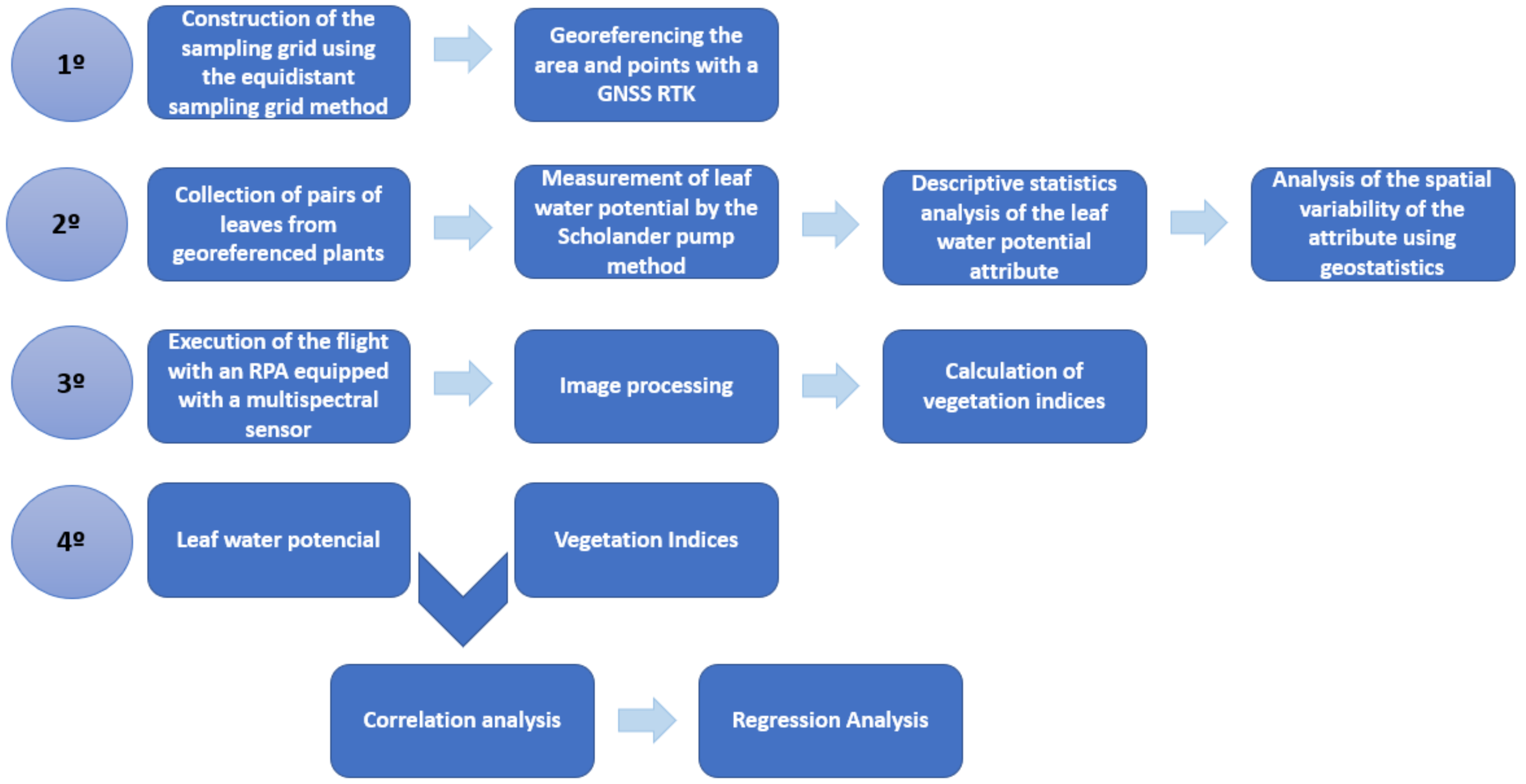
2.1. Workflow

The workflow of this research (Figure 1) was divided into four stages, the first stage being associated with the construction of the sampling mesh and georeferencing of the area and points to be collected, and the second stage being defined as the collection of leaves from the georeferenced plants to obtain the water potential. The third step was defined by the execution of the flight with a multispectral sensor coupled to the RPA, and the fourth step was the correlation analysis and linear regression between the leaf water potential and the calculated vegetation indices.

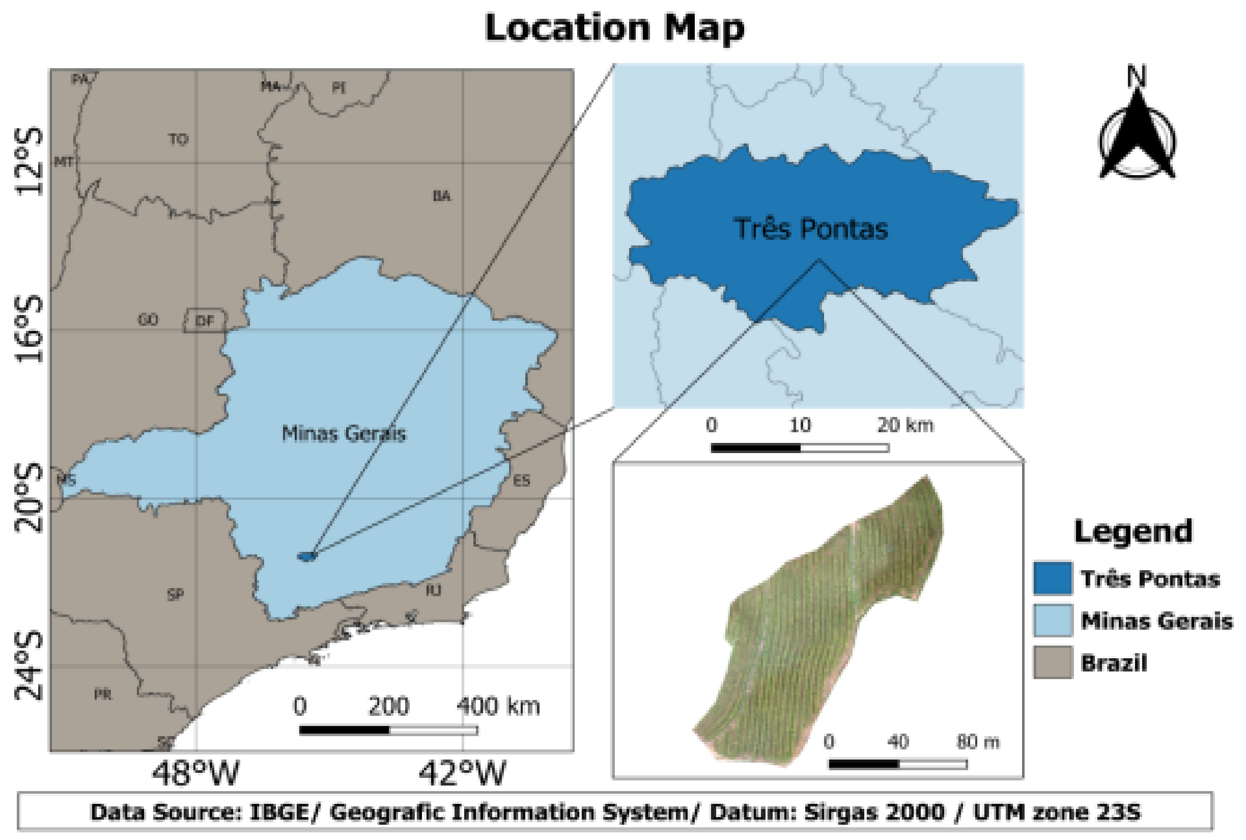
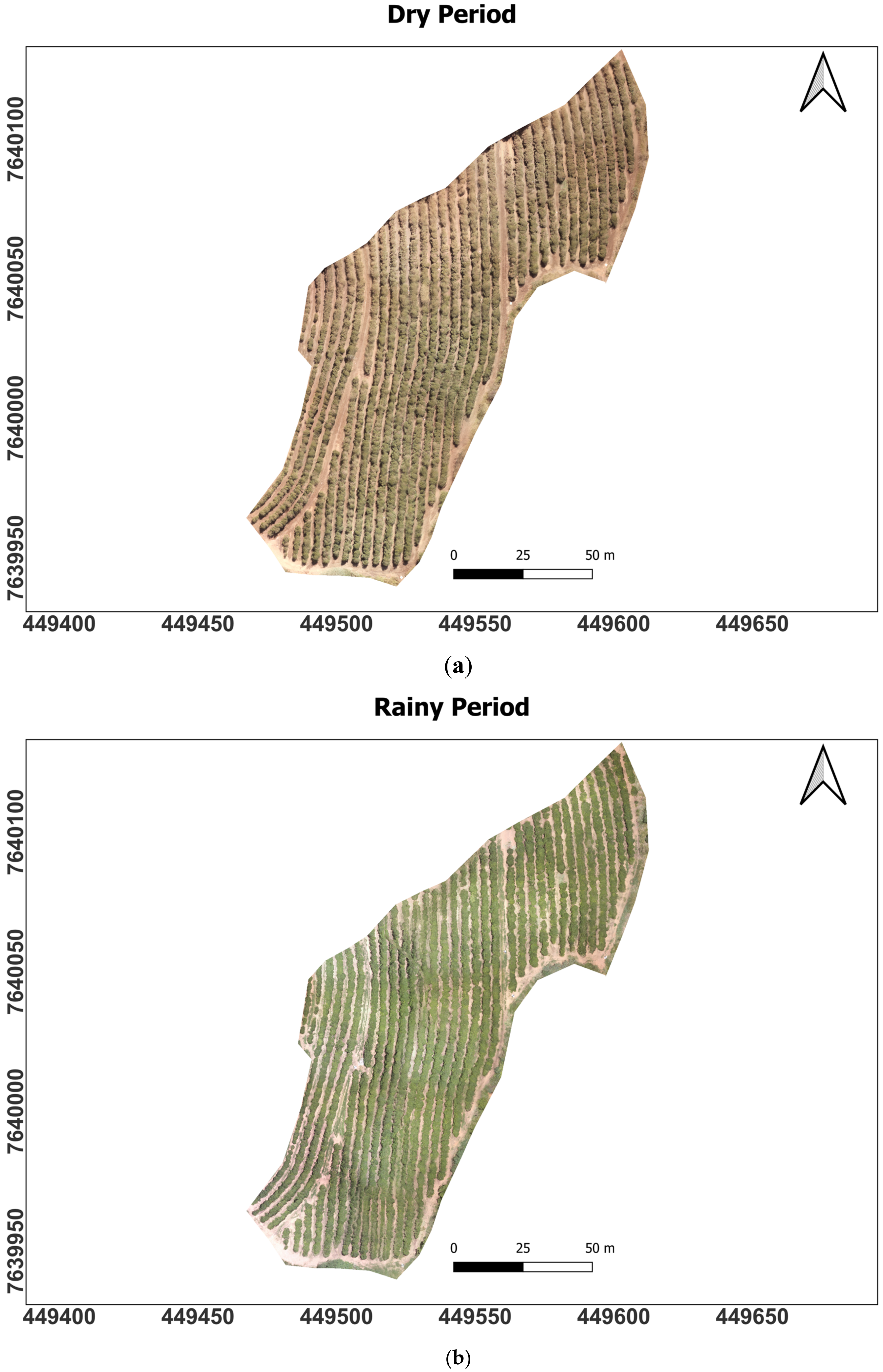
2.2. Description of the Study Area

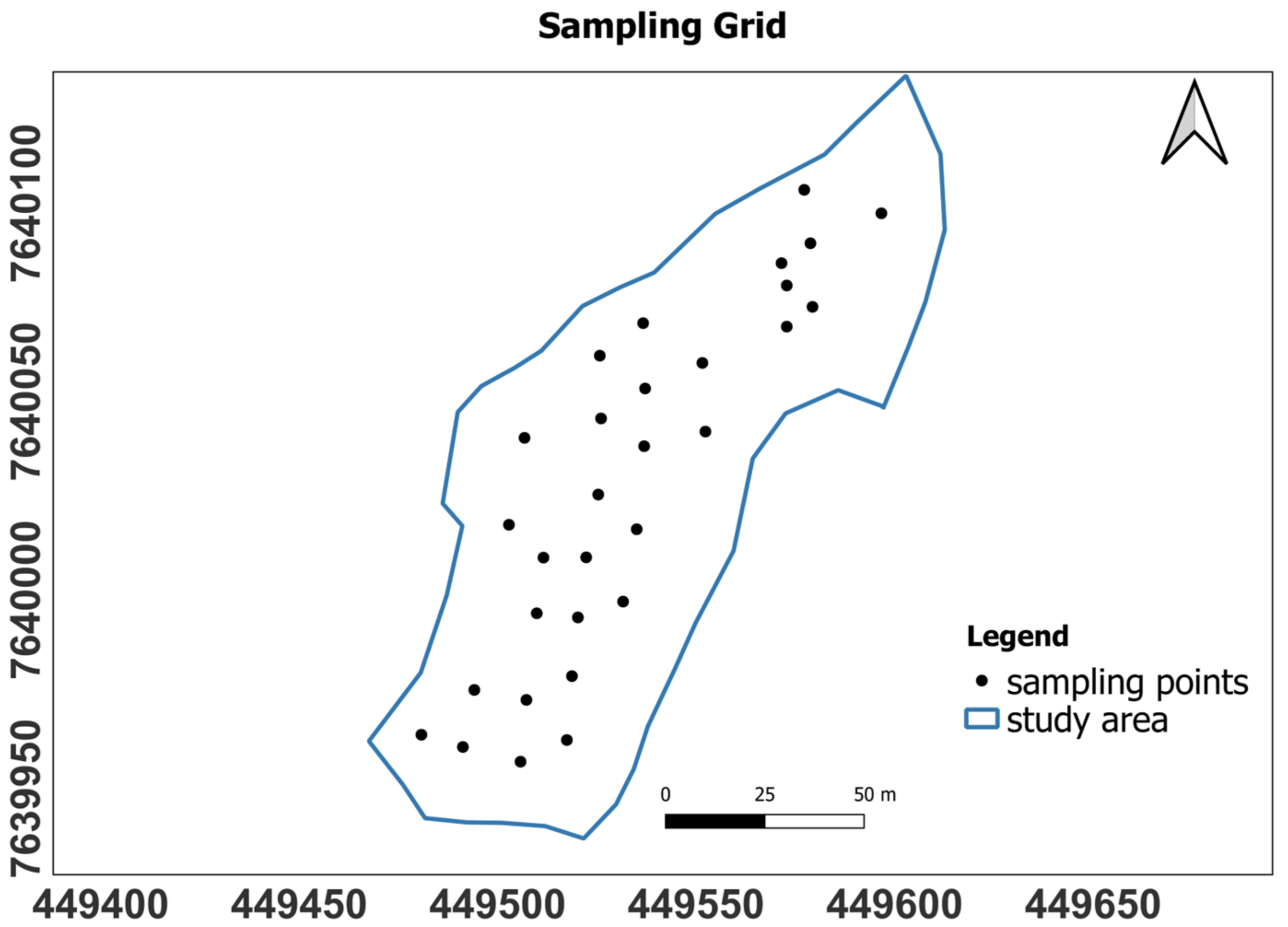
The study was conducted in a coffee plantation of the Experimental Field of the Minas Gerais Agricultural Research Company (EPAMIG, as abbreviated in Portuguese), located in the municipality of Três Pontas in the southern region of the state of Minas Gerais, Brazil, at an altitude of 905 m and a Universal Transverse Mercator (UTM) coordinate system position of S 7640030.4 and E 449531.5, Zone 23K. This municipality has an average annual temperature of 20.3 °C and an average annual rainfall of 1429 mm. The soil in this area is classified as oxisol.

The area of the experiment comprised 1.2 ha of a coffee plantation of the species Coffea arabica L. of the Topázio MG 1190 cultivar. This crop was established in 1998 with spacings between rows of 3.70 m and between plants of 0.70 m (Figure 2).

2.3. Sampling Grid

The sampling grid was prepared with QGIS software, version 3.4.8, and 30 sampling points representing a sampling density of 25 points per hectare were laid out (Figure 3). The contouring of the area and the georeferencing of the sampling points were performed using a TRIMBLE RTK Model R8 global navigation satellite system (GNSS).

The sampling grid considered the cartographic projection of UTM Zone 23 K and WGS 84 DATUM, which consisted of 30 sampling points, with each point represented by a plant that was duly numbered and marked with zebra tape. Two field data collections were performed, one in the dry season on 11 August 2020 and the other in the rainy season on 27 January 2021. Collections were performed to evaluate the water status of the crop in these two periods.

Table 1. Climatological data for the dates of sample collection.

Collection Period	Mean Monthly Temperature (°C)	Date of Last Rainfall	Amount of Last Rainfall (mm)
Dry (August 2020)	19.3	31/05/20	20 mm
Rainy (January 2021)	23.9	20/01/21	115 mm

Source: COOXUPÉ (2020, 2021).

shows the climatological data for both collection dates. These data came from the meteorological station of a farm 15 km away from the EPAMIG experimental field in Três Pontas. These climatological data were obtained from the database of the system of the Regional Cooperative of Coffee Growers in Guaxupé LTDA (COOXUPÉ, as abbreviated in Portuguese).

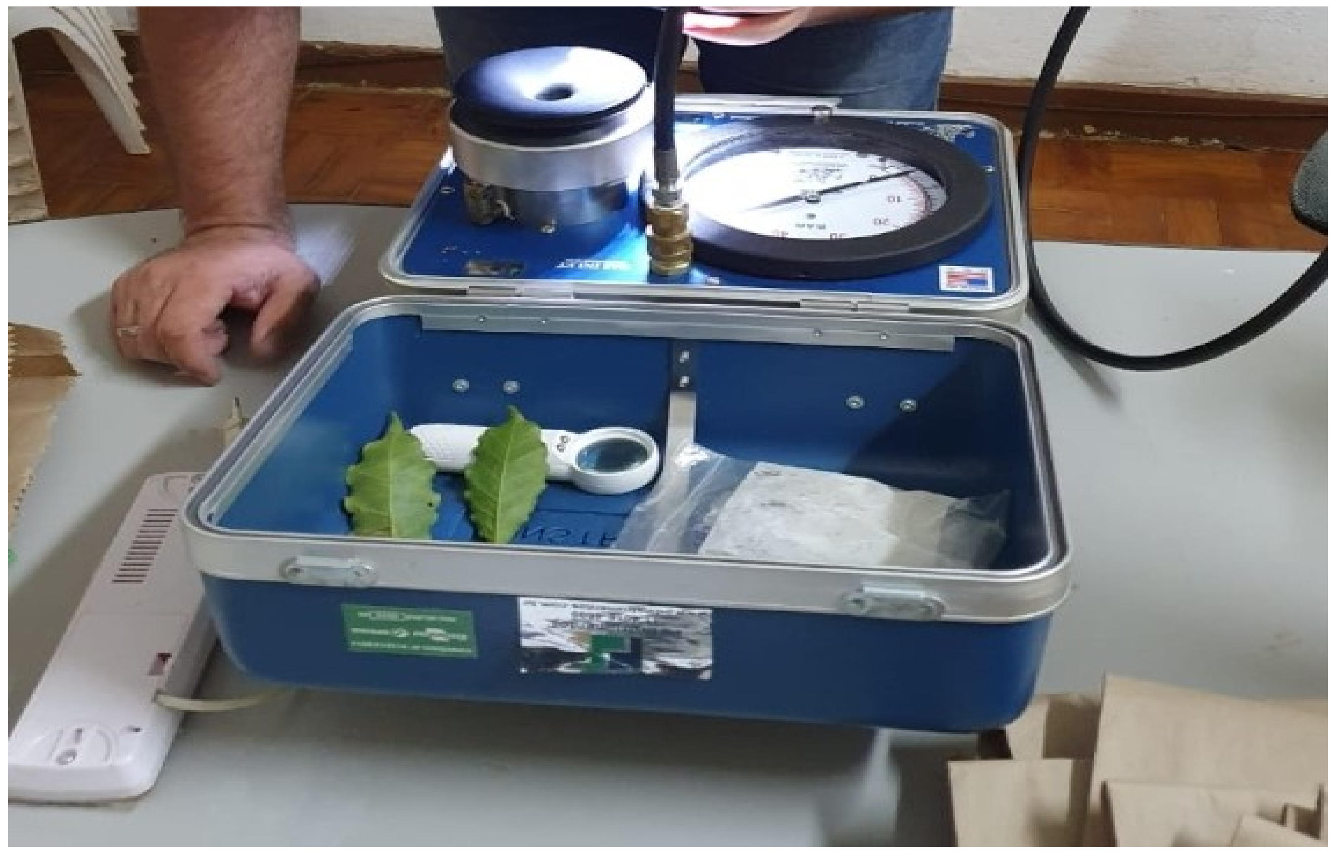
2.4. Leaf Water Potential Collection

Scholander’s pressure pump method was used to collect leaf water potential [19]. The collections were carried out around 4:30 in the morning. A total of 90 leaves were collected, with 3 leaves from each georeferenced plant. These leaves were collected from the middle third of each plant. Each set of 3 leaves was stored in a plastic bag that was properly closed and contained the number of the georeferenced plant.

The leaf water potential was assessed using the Scholander pressure bomb immediately after collection from each georeferenced plant (Figure 4).

This method consists of placing the leaf inside a cylinder so that its petiole stays out by passing it through a small rubber-coated hole in a gas-proof lid. Pressure is gradually supplied to the cylinder chamber until the first sign that the sap is being forced out of the exposed end of the petiole; this is when the gas injection (inert nitrogen) should be interrupted and the manometer should be read. The value on the manometer represents the xylem pressure potential in MPa (megapascals), where the solute or osmotic potential is considered negligible.

2.5. Geostatistical Analysis

Semivariograms were used to analyze the spatial dependence of the leaf water potential. The semivariance is classically estimated by Equation (1) according to [20]:

$$\widehat{\gamma } \left(h\right)=\frac{1}{2 N\left(h\right)} {\displaystyle \sum }_{i=1}^{Ni=\left(h\right)}[Z (x_i)-Z \left(x_i+h\right)]²$$

(1)

where N(h) is the number of experimental pairs of observations Z(xi) and Z(xi + h), separated by a distance h. The semivariogram is represented by the graph $\widehat{\gamma }$(h) versus h. From the fitting of a mathematical model to the calculated values of $\widehat{\gamma }$(h), the coefficients of the theoretical model are estimated for the semivariogram, called the nugget effect (C0), sill (C0 + C1), and range (a), as described by [21].

For this study, the ordinary least squares (OLS) method and spherical, exponential, and Gaussian models were used. These models were chosen according to the fit presented for each attribute studied. To verify whether the fits for each model meet the requirements of cross-validation, the mean error (ME) was calculated according to [22]. The ME should have the closest possible value to zero.

With the adjustment of the semivariograms, after the identification of the spatial variability, the data were interpolated by ordinary kriging. Thus, the variable was estimated in places where it was not sampled, which allowed us to visualize its distribution in space in the form of thematic maps.

The calculation of the degree of spatial dependence (DSD) of the variables followed the classification proposed by [23]. In this classification, the authors point out that there is strong spatial dependence when the semi variogram shows a nugget effect equal to or less than 25% of the sill, moderate spatial dependence when this ratio is between 25% and 75%, and weak spatial dependence when it is greater than 75%.

The geoR package installed in the free statistical software R was used for geostatistical analysis and for the creation of the thematic maps [24].

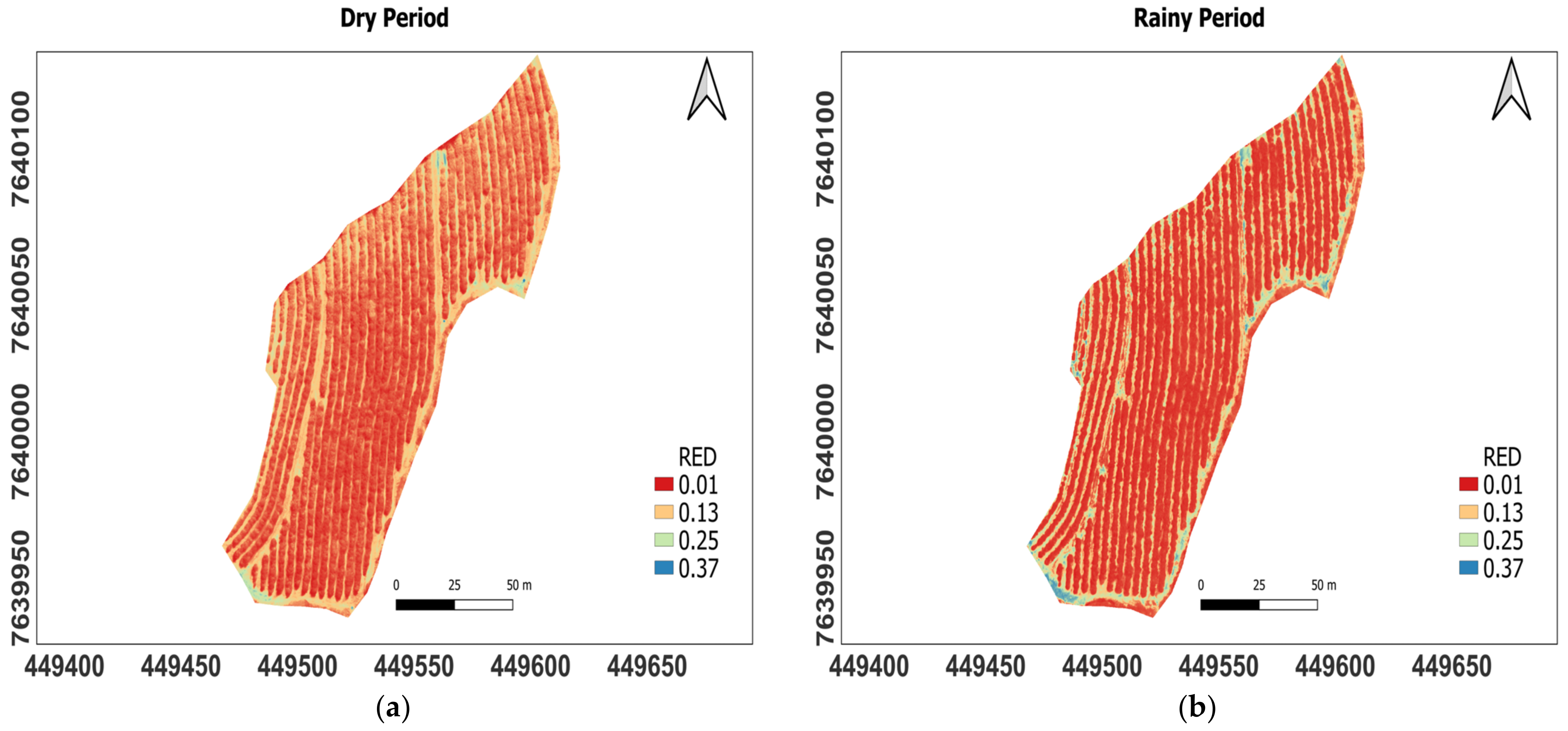
2.6. Image Acquisition and Processing

The set of images was acquired using a senseFly model EBee SQ remotely piloted aircraft. This aircraft has the following characteristics: fixed wing, wingspan of 110 cm, nominal radio range of 3 km, cruising speed of 40–110 km/h, wind resistance of up to 45 km/h (12 m/s), electric motor, maximum payload of 1.1 kg (including camera and batteries), and a flight autonomy of up to 55 min.

The aircraft was equipped with a Parrot camera (Sequoia model) with a high-resolution red–green–blue (RGB) sensor with a focal length of 4.88 mm. This camera also has four monochromatic sensors for the spectral bands: green (550 ± 40 nm), red (660 ± 40 nm), near infrared (NIR) (790 nm ± 40 nm), and red edge (735 ± 40 nm). The resolution is 1280 × 960, with a pixel size of 3.75 μm and focal length equal to 3.98 mm; the ground sample distance (GSD) is 6.8 cm at a flight height of 50 m (above ground level—AGL), which was adopted for the study described.

In addition to the RGB and monochromatic sensors, the Sequoia has a luminosity sensor to correct the influence of the sun by obtaining data with radiometric corrections. This sensor records not only the current lighting, but also the location of the center of the photo and inertial data.

The planning and execution of the flight was performed through the base station, which was developed by the same aircraft manufacturer (senseFly) with the following set: the software eMotion, responsible for the flight scheduling and execution of the aircraft path, and a transmitting antenna allowing the real-time monitoring of the overflight, as well as the sending of landing commands, changes in direction, and acquisition of images. The flight plan followed the parameters shown in

Table 2. Flight planning parameters.

Camera	Parrot Sequoia
Resolution of the RGB Camera	16 megapixels
Resolution of the Multispectral Camera	1.2 megapixels
Focal Length	3.98 mm
Vertical Cover	70%
Horizontal Cover	70%
Spatial Resolution	6.8 cm
Flight Altitude	50 m
Speed	12 m/s

.

Image processing was performed using the software Pix4DMapper. Digital processing consisted of phototriangulation of the image blocks, with obtainment of the exterior and interior orientation parameters of the images, generation of the point cloud, production of the digital surface model (DSM), and generation of the orthomosaic. Five control points were distributed evenly throughout the property to perform the phototriangulation of the images. The points were surveyed with the aid of a Trimble R8 model GNSS of dual frequency in real-time kinematic (RTK) mode with an accuracy of less than 1 mm in a 1 Hz band.

Next, the radiometric correction of the orthomosaics was performed, i.e., the conversion of the values into digital numbers (DNs) for the surface reflectance. This processing was also performed in Pix4DMapper, with resources from Parrot Sequoia. Before the flight, the radiometric calibration of the camera was performed using a reference plate. By using the values of this plate, the software can calibrate and correct the reflectance of the image considering the lighting characteristics at the time of flight.

2.7. Vegetation Indices

Table 3. Vegetation indices calculated from high-resolution images.

Index	Acronym	Equation	Reference
Normalized Difference Vegetation Index	NDVI	$\frac{NIR+RED}{NIR-RED}$	[25]
Normalized Difference Water index	NDWI	$\frac{G-NIR}{G+NIR}$	[26]
Enhanced Vegetation Index 2	EVI2	$2.5\ast \frac{NIR-RED}{\left(NIR+2.4\ast RED+1\right)}$	[27]
Normalized Difference Red Edge	NDRE	$\frac{NIR-RED Edge}{NIR+RED Edge}$	[28]
Clorophyll Vegetation Index	CVI	$\frac{NIR}{GREEN}\ast \frac{RED}{GREEN}$	[29]
Green Normalized Difference Red Edge	GNDVI	$\frac{NIR-GREEN}{NIR+GREEN}$	[30]
Canopy Chlorophyll Content Index	CCCI	$\frac{NDRE}{NDVI}$	[28]
Green Ratio of Vegetation Index	GRVI	$\frac{NIR}{GREEN}$	[31]
Modified Simple Ratio	MSR	$\frac{\left(\frac{NIR}{RED}\right)-1}{\left(\sqrt{\frac{NIR}{RED}}\right)+1}$	[32]
Infrared Percentage Vegetation Index	IPVI	$\frac{\mathrm{NIR}}{\mathrm{NIR}+\mathrm{RED}}$	[33]
Soil-Adjusted Vegetation Index	SAVI	$\frac{\left(1+L\right)\left(NIR-RED\right)}{L+NIR+RED}$	[34]
Modified Soil-Adjusted Vegetation Index 2	MSAVI	$\frac{[2NIR+1-{\left({\left(2NIR+1\right)}^2-8\left(NIR-RED\right)\right)}^{0.5}]}{2}$	[35]
Optimized Soil-Adjusted Vegetation Index	OSAVI	$\frac{\left(NIR-RED\right)}{\left(NIR+RED+0.16\right)}$	[36]
Green Clorophyll Index	CIgreen	$\left(\frac{NIR}{GREEN}\right)-1$	[37]
Red-edge Clorophyll Index	CIrededge	$\left(\frac{NIR}{RED EDGE}\right)-1$	[37]

shows the vegetation indices that were calculated from the high-resolution spectral bands obtained by the multispectral sensor coupled to the RPA.

2.8. Correlation Analysis and Linear Regression

To identify the vegetation indices with the best correlation with the water potential attribute, data correlation and linear regression techniques were performed where the correlation summarized the degree of the relationship between two variables (X and Y, for example). Conversely, regression results in a mathematical equation describing the relationship between variables.

To perform the simple linear regression, the samples extracted from each index (containing the mean reflectance value of each point) were used as the dependent variable, and the independent variables were represented by the water potential data of the leaves collected in the field.

To collect the dependent variables, polygonal samples were taken from the georeferenced points. These polygons were constructed with a buffer, i.e., each sample had a radius of 0.20 m (20 cm). Samples were obtained using the zonal statistics tool, which calculates the mean reflectance value of pixels within a polygon. For each georeferenced point, 30 mean reflectance values were obtained for each vegetation index studied.

The mean value of each point and each calculated index was exported to a table in which linear regression operations were performed using the Excel program, and the values of the Pearson correlation coefficient (R) and coefficient of determination were obtained, in addition to the F hypothesis tests, to test the significance of each hypothesis. Considering that Ho: ρ = 0, the hypotheses used in this research were:

Hypothesis 0 (H0).

ρ = ρ₀ null hypothesis;

Hypothesis 1 (H1).

ρ ≠ ρ₀ alternative hypothesis.

The correlation between the variables is given by the linear coefficient of Person (R) calculated from Equation (2). The value of R is always in the range of −1 to 1.

$$R=\frac{n{{\displaystyle \sum }}_{i=1}^n{x}_i{y}_i-{{\displaystyle \sum }}_{i=1}^n{x}_i{{\displaystyle \sum }}_{i=1}^n{y}_i}{\sqrt{n{{\displaystyle \sum }}_{i=1}^n{x}_i²-({{\displaystyle \sum }}_{i=1}^n{x}_i)² }\sqrt{n{{\displaystyle \sum }}_{i=1}^n{y}_i²({{\displaystyle \sum }}_{i=1}^n{y}_i)²}}$$

(2)

The interpretation of Pearson’s correlation coefficient is described in

Table 4. Interpretation of Pearson’s correlation coefficient.

Correlation Coefficient	Correlation
Rxy = 1	Perfect Positive
0.8 ≤ Rxy < 1	Strong Positive
0.5 ≤ Rxy < 0.8	Moderate Positive
0.1 ≤ Rxy < 0.5	Weak Positive
0 ≤ Rxy < 0.1	Very Weak Positive
0	Null
−0.1 ≤ Rxy < 0	Very Weak Negative
−0.5 ≤ Rxy < −0.1	Weak Negative
−0.8 ≤ Rxy < −0.5	Moderate Negative
−1 ≤ Rxy < −0.8	Strong Negative
Rxy = −1	Perfect Negative

Source: Adapted Ref. [38].

.

The relationship between these variables is represented by a mathematical model, that is, an equation that associates the dependent variable with the independent variables. The model is called simple linear regression. From the linear regression, the determination coefficient is obtained, which is expressed by Equation (3).

$$R^2=\frac{\sum \left({\widehat{y}}_i-y\right)²}{\sum \left(y_i-\overline{y}\right)²}=\frac{variation explained by the model}{total variation}$$

(3)

The coefficient of determination is a descriptive measure of the proportion of variation in the independent variable that can be explained by variations in the dependent variable according to the specified regression model. The closer the coefficient of determination is to 1, the better the degree of explanation of the variation in Y as a function of the variable X. It is always a positive measure and is obtained in simple linear regression by increasing the squared Pearson’s correlation coefficient.

The F test of hypotheses at the 95% confidence level was used to determine whether the variability between the group means was greater than the variability of the observations within the groups. If this proportion is sufficiently large, it can be concluded that not all means are equal.

3. Results

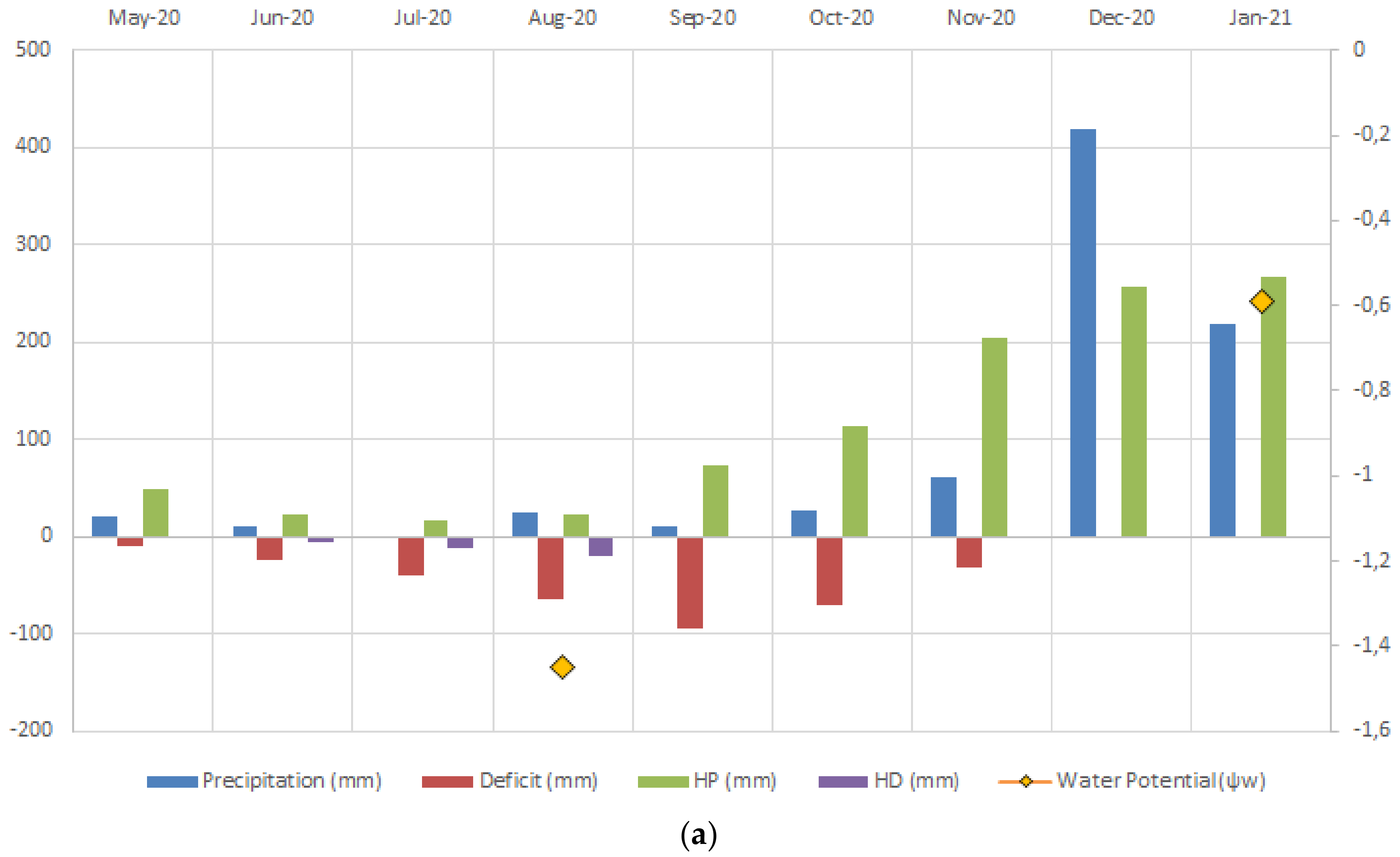
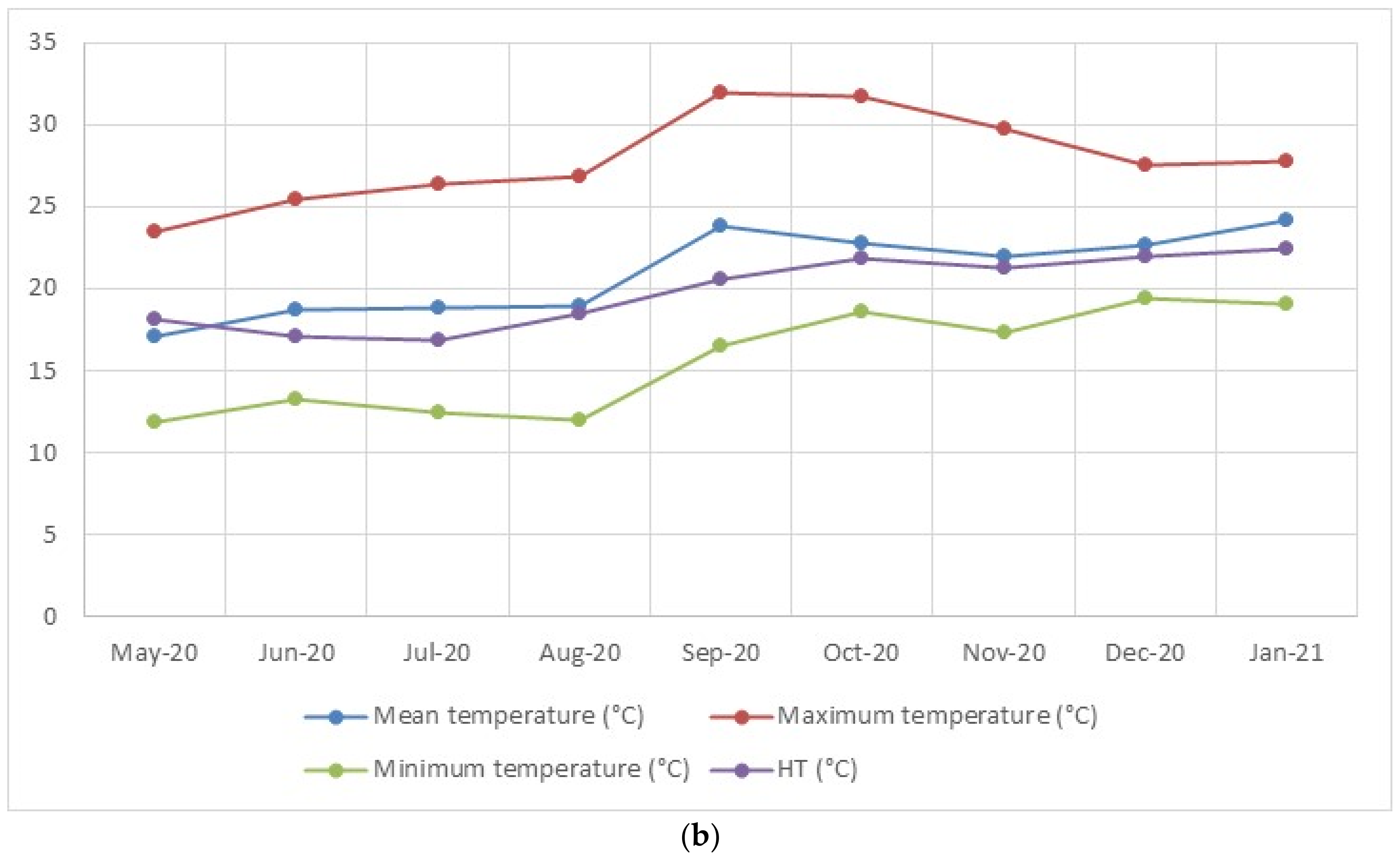
3.1. Hydrological Conditions

Figure 5a,b represent the graphs containing the climate data during the interval that precedes the collections in the dry period (May 2020) until the collection of the rainy period (January 2021). Figure 5a represents the precipitation and deficit data for the municipality of Três Pontas, as well as the average leaf water potential data obtained in the two field collections (August 2020 and January 2021), and to complement these data, the mean of historical series of precipitation and deficit were added. Figure 5b represents the temperature distribution graph (mean, maximum, minimum and historical average temperature 1991–2021) within the range from May 2020 to January 2021.

3.2. Descriptive Statistic

The descriptive statistics of leaf water potential (Ψw, in MPa) are shown in

Table 5. Descriptive statistics for the variable Ψw (MPa) for the dry and rainy seasons.

Period	Variable			Descriptive Statistics
		Min	Max	Md	Mean	Var	SD	CV (%)
Dry	Ψw MPa (2020)	−3.3	−0.5	1.15	1.45	0.61	0.78	53
Rainy	Ψw MPa (2021)	−0.8	−0.3	0.6	0.59	0.01	0.10	17

Min = minimum value; Max = maximum value; Md = median; Mean = mean; Var = variance; SD = standard deviation; and CV = coefficient of variation (%).

. The first indicators of data heterogeneity are high values of the coefficient of variation (CV). The authors of [39] state that the variability of an attribute can be classified according to the magnitude of its CV, which according to the authors is low when it is less than 10%; moderate when it is in the range between 10 and 20%; high when it is between 20 and 30%; and very high when it is above 30%.

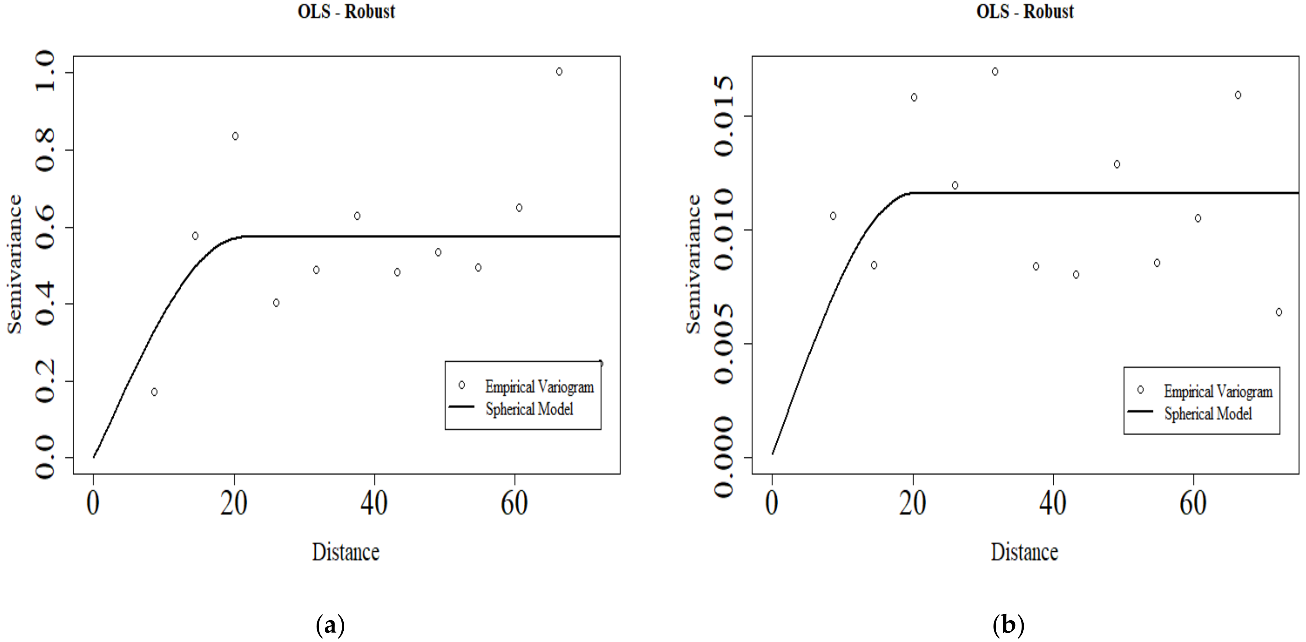
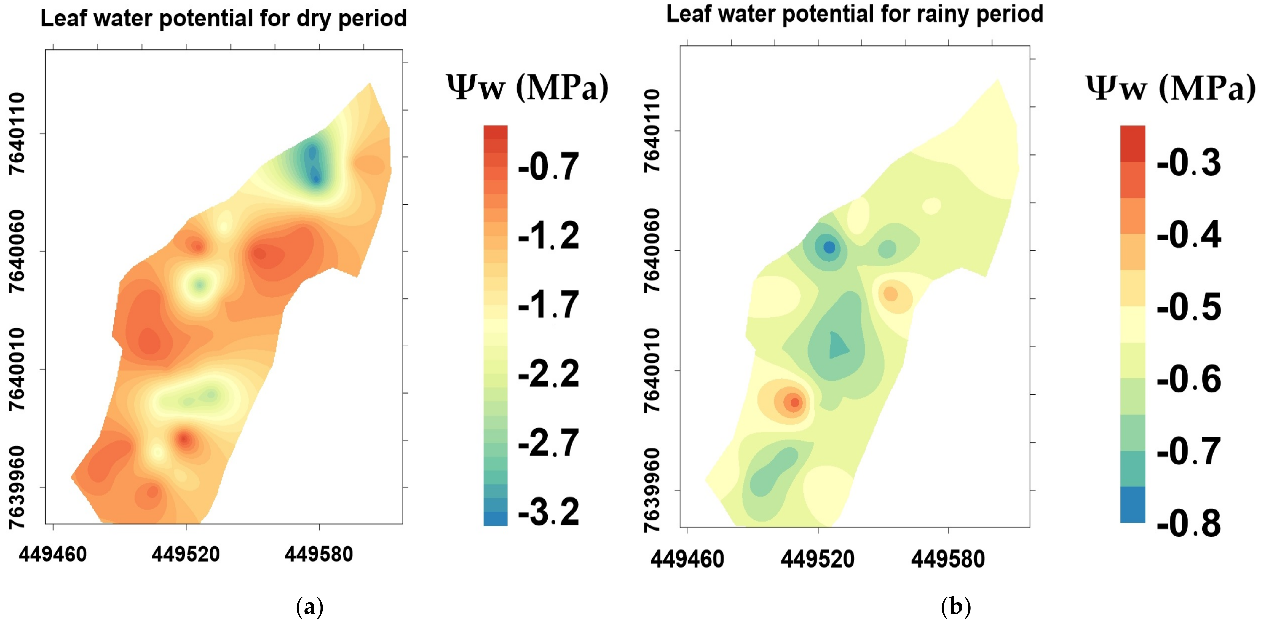
3.3. Geostatistical Analysis

Table 6. Parameters for fitting the spherical and exponential semivariogram models of the variables evaluated by the OLS method.

Variable	Period	Model	C0	C1	C0 + C1	A	DSD	ME
Ψw (MPa)	Dry	Sph	0.10	0.40	0.50	20.00	strong	0.00
	Rainy	Sph	0.01	15.00	15.01	0.06	strong	0.00

shows the adjustment parameters of the semivariograms. Of the evaluated models (spherical, exponential, and gaussian), the spherical semivariogram model had the lowest ME for both evaluated periods; thus, it was the fit model chosen. The authors of [40] state that there is a predominance of the spherical mathematical model for studies in soil science.

The leaf water potential had a range of 15 m for both the sampling in the dry season and the sampling in the rainy season, i.e., Ψw had a similar area of influence for both sampling periods. According to the classification of [23], the variable Ψw showed a strong degree of dependence for both periods evaluated. The semivariograms fitted for the water potential variable are shown in Figure 6a,b.

Figure 7a,b represent the spatial variability maps of Ψw made by kriging interpolation.

3.4. Regression and Correlation Analysis

The morphophysiological responses of plants under stress conditions alter the optical properties of coffee plants and the reflectance patterns of the leaves and canopies. Researchers in the areas of orbital RS have developed studies to evaluate water stress in coffee plantations [41,42].

Ref. [43] state that agricultural sectors have widely used RPA for conveniently and efficiently detecting water stress. The evaluation of water stress using vegetation indices obtained by high-resolution images is found in the studies of [44,45,46,47]. These authors state that the use of high-resolution images with the application of vegetation indices is a valuable tool for evaluating water stress in crops, but none of these studies evaluated water deficit in coffee plantations.

A linear regression and correlation analysis was performed to evaluate the relationship between the leaf water potential collected in the field and the values obtained by calculating the 15 vegetation indices and the 4 bands obtained by the multispectral sensor.

Table 7. Correlation analysis between the leaf water potential and multispectral bands and vegetation indices.

Spectral Bands and Vegetation Indices	Ψw (MPa)
	Dry	Rainy
RED	0.3188 ns	0.3993 **
NIR	0.0489 ns	0.1220 ns
RED EDGE	0.1921 ns	0.0493 ns
GREEN	0.2852 ns	0.1424 ns
NDVI	0.1768 ns	0.3010 ns
NDWI	0.0905 ns	0.2620 ns
EVI2	0.0663 ns	0.1663 ns
NDRE	0.2870 ns	0.3263 ns
CVI	0.1742 ns	0.0865 ns
GNDVI	0.0905 ns	0.2620 ns
CCCI	0.2451 ns	0.3356 ns
GVI	0.1113 ns	0.2691 ns
MSR	0.1768 ns	0.3010 ns
IPVI	0.1768 ns	0.0996 ns
SAVI	0.0442 ns	0.1710 ns
MSAVI	0.1012 ns	0.1576 ns
OSAVI	0.1035 ns	0.2090 ns
CI green	0.1113 ns	0.2691 ns
CI red edge	0.2906 ns	0.3313 ns

Ψw-water potential; **—significant at the 5% probability level (p < 0.05) and ns—not significant.

shows the Pearson correlation analyses between the mean of the samples collected from the multispectral bands (red, NIR, red edge, and green) and the vegetation indices in relation to the data collected in the field for the dry season and rainy season. An F test of the hypotheses was performed to evaluate the significance of the correlation at a level of 0.05 (5%).

During the dry season, no correlations were found between water potential in relation to the multispectral bands and the vegetation indices for the vegetation samples using the F test for the hypotheses. For the rainy season, there was a significant correlation of 0.3993 (39.93%) between the water potential and the multispectral red band.

Through the significant correlation presented by the red band and the water potential variable, the parameters of the linear equation obtained by the analysis of variance are represented in

Table 8. Linear regression analysis parameters.

Variable	Period	Spectral Band or Index	β0	β1	R²
Ψw (MPa)	Rainy	RED	−0.0402	−0.0134	0.1595

Ψw—water potential; β0—intercept; β1—angular coefficient; R²—determination coefficient.

and indicate an R² value of 0.1595 or 15.95%.

Figure 8 shows the RGB orthomosaic of the study area obtained for both the dry season (Figure 8a) and the rainy season (Figure 8b). The crop shows very distinct visual characteristics; there is a greater presence of dust on the coffee plant in the dry season, and there is a green, clean, and vigorous plant in the rainy season.

From the verification of the significant correlations between leaf water potential and the vegetation indices, Figure 9a,b represent the maps of the red multispectral band for both the dry and rainy periods, in which there was a significant correlation with the water potential data collected in the field.

This spectral band ranged from the lowest value of 0.01 to the highest value of 0.37; for the dry season, there was a greater predominance in the range of 0.01 to 0.13, and for the rainy season, the highest predominance was in the value of 0.01.

Visually, this band did not present very different characteristics from one period to another; a common characteristic between them occurred at the border of the area, where there were some points where the band had a reflectance value of 0.25.

4. Discussion

4.1. Variation in Climatic Conditions and Descriptive Analysis of Leaf Water Potential

Evaluating the climate variation within the period from May 2020 to January 2021 (Figure 5a), it is observed that in the interval comprising the dry period (May 2020 to August 2020), precipitation was lower and the deficit was greater in relation to the data presented by the historical series, which justifies the low values of leaf water potential. Within the range from November 2020 to January 2021 (rainy period), only the month of December presented precipitation greater than that established for the historical series, and within this period there were no deficits.

The average monthly temperatures from May 2020 to January 2021 were higher than the averages presented by the historical series (Figure 5b) with the exception of the month of May. The relationship between temperature and precipitation influences the evapotranspiration of the coffee tree and can be evaluated by calculating the climatological water deficit; it is observed that the accumulated water deficit for this period from May 2020 to January 2021 was 336 mm, and the month that presented the greatest water deficit was the month of September, which is justified by the second highest average temperature of the period (May 2020 to January 2021) behind only the month of December.

For the dry season, Ψw had a CV of 53%, and for the rainy season it had a CV of 17%, presenting very high and moderate heterogeneity, respectively, according to the criteria of [39]. Taking into account the negative sign for the water potential reading in MPa, the lowest value occurred in the dry season (−3.3 MPa), whereas the highest value occurred in the rainy season (−0.3 MPa). The leaf water potential showed mean values of −1.45 MPa for the dry season and −0.59 MPa for the rainy season. In [48], water potential values between −1.5 MPa and −3.0 MPa represent moderate and severe water deficits, respectively.

Thus, the mean water potential values collected in the dry and rainy periods were not within the water deficit interval. Statements by [49,50] indicate maximum values of −1.5 MPa for coffee plants without irrigation in the field under normal climate conditions, suggesting that this is a limiting value for the nonoccurrence of physiological disturbances in the plant under normal cultivation conditions.

The moderate water-deficit severity reflected in the water potential for the dry period may be related to the absence of rainfall in this period, as observed in Table 1, where the last 20 mm rainfall occurred 74 days (31 May 2020) before the date of sample collection. The highest values of this attribute evaluated in the rainy season were observed when there was a 115 mm rainfall seven days before the date of sample collection.

Some authors have presented water potential results similar to those found in this study. For example, Ref. [51] found a mean water potential value of–1.17 MPa for the cultivar of the current study (Topázio MG 1190); Ref. [51] found mean water potential values of −1.25 MPa; and the mean value was −0.79 MPa for a coffee cultivation area during the rainy season, which was below the severity interval mentioned by [52], as occurred in this study.

4.2. Geostatistical Analysis

Leaf water potential for the dry season (Figure 7a) ranged from the lowest value of −3.2 MPa to the highest value of −0.7 MPa; the predominance of water potential for this period was in the range between −1.7 and −1.2 MPa (tones from creamy yellow to light orange), with part of these values belonging to the range of severity of moderate water deficit [48]. The lowest values, in the range of −3.2 to −2.7 MPa, were observed northwest of the area (shades from blue to green). The leaf water potential for the rainy season (Figure 7b) ranged from the lowest value (−0.8 MPa) to the highest value (−0.3 MPa) and, according to [53], this range was within the range in which plants do not present water deficit.

4.3. Regression and Correlation Analysis

The morphophysiological responses of plants under stress conditions alter the optical properties of coffee trees and the reflectance patterns of leaves and canopies. Researchers in the areas of orbital remote sensing have developed work to assess water stress in coffee growing [41,42].

By identifying water balance variables and their relationship between vegetation indices obtained by the MODIS sensor (Terra satellite) for coffee growing, Ref. [40] evaluated the NDVI and EVI vegetation indices obtained by the MODIS sensor (Terra satellite). The authors claim that the relationships between climate–topological water balance variables and vegetation indices were verified, but with weak statistical correlation.

Aiming to estimate the water potential of the leaf through the evaluation of vegetation indices calculated through Landsat−8 images, [41] states that a quadratic algorithm that uses the Normalized Difference Vegetation Index (NDVI) performed better, showing a correlation coefficient (R²) of 0.82.

The authors [43] state that agricultural sectors have used RPA widely for convenience and efficiency in detecting water stress.

Preparing a literature review, Ref. [44] valuated the application of different types of RPA and remote sensors and compared their performance with field truth for different crops. The results of this review indicate that the NDVI, TCARI/OSAVI and PRI showed positive correlations related to water stress.

The authors of [45] assessed the prospects for improving agricultural and water productivity through remotely piloted aircraft. The authors aimed to build a literature review where they summarized the use of RPA in smallholder agriculture in developing countries. The review highlights the role of the NDVI index obtained by RPA in assessing crop health, evapotranspiration, water stress and disaster risk reduction. Based on the results, the authors state that water stress indices (CWSI and WDI) provide a better option for agricultural water management and adaptation to climate change.

The authors of [46], using images from a remotely piloted aircraft equipped with a multispectral sensor, aimed to identify water stress in maize under different levels of irrigation. Through high-resolution multispectral images, the authors found nine vegetation indices to be related to water stress. Based on the results, the authors observed R² values of 0.47 and 0.50 for TCARI/RDVI and TCARI/SAVI in the reproductive and maturation stages, respectively, and 0.81 and 0.80 for TCARI/RDVI and TCARI/SAVI in the late reproductive and maturation stages, respectively.

The authors of [47] investigated whether the water deficit index (WDI) based on images from remotely piloted aircraft could provide accurate maps of water stress in crops at different stages of growth. For this study, the author evaluated two crops grown with spring barley using thermal and RGB cameras, which were mounted in the RPA. Based on the results, the authors concluded that WDI maps can potentially serve as water stress maps.

The authors mentioned above highlight in their studies the various applications of RPAs in agriculture as well as the assessment of water stress in different crops, but during the development of this work, no study was found that assessed water stress in coffee crops through high-resolution images.

Despite the positive correlation between leaf water potential and the red spectral band, the R² value was not significant (0.1595). A justification for this fact is the difference between data collection methodologies. Three leaves were collected from each georeferenced plant to determine the water potential obtained in the field, and were subjected to the Scholander pressure bomb. Regarding the sampling performed to obtain the vegetation indices, polygons 20 cm in diameter whose perimeter contained more than three leaves of coffee plants were sampled; this perimeter may contain healthy and unhealthy leaves, which directly interferes with the mean values and does not follow a specific sampling pattern, as is the case of field sampling.

Another justification for the results presented in this study may be linked to the dust layer present on the coffee plant in the dry period. The dust layer directly affects the reflectance value of the multispectral bands, serving as a basis to calculate the vegetation indices and to estimate water potential using the Scholander pressure bomb, which requires that clean leaves are inserted in the pressure chamber, i.e., these leaves did not represent the actual field conditions under which the images were captured by the sensor coupled to the RPA.

5. Conclusions

The water potential variable showed the spatial variability structure through the calculation of the CV. In turn, the geostatistical analysis showed that the degree of spatial dependence was strong for both periods evaluated. In the correlation analysis between water potential, multispectral bands and vegetation indices, only the red band evaluated in the rainy season showed a significant correlation at 0.3993 (39.93%). Even with a significant correlation between the water potential and the red band for the rainy season, the R² value was low (15.95%) in the linear regression analysis.

The use of the geostatistical tool was efficient for evaluating the spatiotemporal behavior of the water potential variable. Conversely, the use of high-resolution images to evaluate the water conditions of coffee plantations requires better studies, especially regarding sampling, to make this tool more efficient in monitoring and detecting the variability of water conditions and to aid producers in their decision-making in relation to management.

References

1. Furlan, D.A.; De Sousa, E.F.; Mendonça, J.C.; De Souza, C.L.M.; Gottardo, R.D.; De Souza Lima, R.A. Potencial hídrico foliar e desenvolvimento vegetativo do cafeeiro conilon sob diferentes lâminas de irrigação na região e campos dos Goytacazes-RJ. IRRIGA 2021, 26, 13–28. [Google Scholar] [CrossRef]
2. DaMatta, F.M.; Grandis, A.; Arenque, B.C.; Buckeridge, M.S. Impacts of climate changes on crop physiology and food quality. Food Res. Int. 2010, 43, 1814–1823. [Google Scholar] [CrossRef]
3. Silva, A.S.; Lima, J.S.S. Atributos físicos do solo e sua relação espacial com a produtividade do café Arábica. Coffee Sci. 2013, 8, 395–403. [Google Scholar]
4. Da Costa, G.F.; Marenco, R.A. Fotossíntese, condutância estomática e potencial hídrico foliar em árvores jovens de andiroba (Carapa guianensis). Acta Amaz. 2007, 37, 229–234. [Google Scholar] [CrossRef]
5. Cavatte, P.C.; Oliveira, A.G.; Morais, L.E.; Martins, S.C.V.; Sanglard, L.M.V.P.; DaMatta, F.M. Could shading reduce the negative impacts of drought on coffee? A morphophysiological analysis. Physiol. Plant. 2011, 144, 111–122. [Google Scholar] [CrossRef]
6. Ferraz, G.A.E.S.; Da Silva, F.M.; De Oliveira, M.S.; Custódio, A.A.P.; Ferraz, P.F.P. Variabilidade espacial dos atributos da planta de uma lavoura cafeeira. Rev. Ciência Agronômica 2017, 48, 81–91. [Google Scholar] [CrossRef] [Green Version]
7. Carvalho, L.C.L.; Da Silva, F.M.; Ferraz, G.A.S.; Silva, F.C.; Stracieri, J. Variabilidade espacial de atributos físicos do solo e características agronômicas da cultura do café. Coffee Sci. 2013, 8, 265–275. [Google Scholar]
8. Herwitz, S.; Johnson, L.; Dunagan, S.; Higgins, R.; Sullivan, D.; Zheng, J.; Lobitz, B.; Leung, J.; Gallmeyer, B.; Aoyagi, M.; et al. Imaging from an unmanned aerial vehicle: Agricultural surveillance and decision support. Comput. Electron. Agric. 2004, 44, 49–61. [Google Scholar] [CrossRef]
9. Zhou, J.; Pavek, M.J.; Shelton, S.C.; Holden, Z.J.; Sankaran, S. Aerial multispectral imaging for crop hail damage assessment in potato. Comput. Electron. Agric. 2016, 127, 406–412. [Google Scholar] [CrossRef] [Green Version]
10. Zhang, J.; Hu, J.; Lian, J.; Fan, Z.; Ouyang, X.; Ye, W. Seeing the forest from drones: Testing the potential of lightweight drones as a tool for long-term forest monitoring. Biol. Conserv. 2016, 198, 60–69. [Google Scholar] [CrossRef]
11. Johnson, L.F.; Herwitz, S.R.; Lobitz, B.M.; Dunagan, S.E. Feasibility of Monitoring Coffee Field Ripeness with Airborne Multispectral Imagery. Appl. Eng. Agric. 2004, 20, 845–849. [Google Scholar] [CrossRef]
12. Martins, R.N.; Pinto, F.D.A.D.C.; de Queiroz, D.M.; Valente, D.S.M.; Rosas, J.T.F. A Novel Vegetation Index for Coffee Ripeness Monitoring Using Aerial Imagery. Remote Sens. 2021, 13, 263. [Google Scholar] [CrossRef]
13. Oliveira, H.C.; Guizilini, V.C.; Nunes, I.P.; Souza, J.R. Failure Detection in Row Crops From UAV Images Using Morphological Operators. IEEE Geosci. Remote Sens. Lett. 2018, 15, 991–995. [Google Scholar] [CrossRef]
14. Santos, L.M.D.; Andrade, M.T.; Santana, L.S.; Rossi, G.; Maciel, D.T.; Barbosa, B.D.S.; Ferraz, G.A.S. Analysis of flight parameters and georeferencing of images with different control points obtained by RPA. Agron. Res. 2019, 17, 2054–2063. [Google Scholar] [CrossRef]
15. Da Cunha, J.P.A.R.; Neto, M.A.S.; Hurtado, S.M.C. Estimating Vegetation Volume of Coffee Crops Using Images from Unmanned Aerial Vehicles. Eng. Agrícola 2019, 39, 41–47. [Google Scholar] [CrossRef]
16. Dos Santos, L.M.; Ferraz, G.A.E.S.; Barbosa, B.D.D.S.; Diotto, A.V.; Andrade, M.T.; Conti, L.; Rossi, G. Determining the Leaf Area Index and Percentage of Area Covered by Coffee Crops Using UAV RGB Images. IEEE J. Sel. Top. Appl. Earth Obs. Remote Sens. 2020, 13, 6401–6409. [Google Scholar] [CrossRef]
17. Santana, L.S.; Santos, L.M.; Maciel, D.A.; Barata, R.A.P.; Reynaldo, É.F.; Rossi, G. Vegetative Vigor of Maize Crop Obtained through Vegetation Indexes in Orbital and Aerial Sensors Images. Rev. Bras. Eng. Biossistemas 2019, 13, 195–206. [Google Scholar] [CrossRef] [Green Version]
18. Dos Santos, L.M.; Ferraz, G.A.E.S.; Barbosa, B.D.D.S.; Diotto, A.V.; Maciel, D.T.; Xavier, L.A.G. Biophysical parameters of coffee crop estimated by UAV RGB images. Precis. Agric. 2020, 21, 1227–1241. [Google Scholar] [CrossRef]
19. Scholander, P.F.; Bradstreet, E.D.; Hemmingsen, E.A.; Hammel, H.T. Sap pressure in vascular plants: Negative hydrostatic pressure can be measured in plants. Science 1965, 148, 339–346. [Google Scholar] [CrossRef]
20. Vieira, S.R. Geoestatística em Estudos de Variabilidade Espacial do solo. Tópicos Especiais em Ciências do solo. Sociedade Brasileira de Ciência do Solo, 1st ed.; Novais, R.F., Alvarez, V.V.H., Schaefer, C.E.G.R., Eds.; Sociedade Brasileira de Ciência do Solo: Viçosa, Brazil, 2000; pp. 1–54. [Google Scholar]
21. Bachmaier, M.; Backes, M. Variogram or semivariogram? Understanding the variances in a variogram. Precis. Agric. 2008, 9, 173–175. [Google Scholar] [CrossRef]
22. Isaaks, E.H.; Srivastava, R.M. An Introduction to Applied Geostatistics; Oxford University Press: Oxford, UK, 1989; p. 413. [Google Scholar]
23. Cambardella, C.A.; Moorman, T.B.; Novak, J.M.; Parkin, T.B.; Karlen, D.L.; Turco, R.F.; Konopka, A.E. Field-Scale Variability of Soil Properties in Central Iowa Soils. Soil Sci. Soc. Am. J. 1994, 58, 1501–1511. [Google Scholar] [CrossRef]
24. Ribeiro Junior, P.J.; Diggle, P.J. GeoR a package for geostatistical analysis. R-News 2001, 1, 14–18. [Google Scholar]
25. Rouse, J.; Haas, R.; Schell, J.; Deering, D. Monitoring Vegetation Systems in the Great Plains with ERTS. In Proceedings of the Earth Resources Technology Satellite Symposium, Washington, DC, USA, 10–14 December 1973; Volume 1, pp. 309–317. [Google Scholar]
26. McFeeters, S.K. The use of the Normalized Difference Water Index (NDWI) in the delineation of open water features. Int. J. Remote Sens. 1996, 17, 1425–1432. [Google Scholar] [CrossRef]
27. Jiang, Z.; Huete, A.R.; Didan, K.; Miura, T. Development of a two-band enhanced vegetation index without a blue band. Remote Sens. Environ. 2008, 112, 3833–3845. [Google Scholar] [CrossRef]
28. Barnes, E.M.; Clarke, T.R.; Richards, S.E.; Colaizzi, P.D.; Haberland, J.; Kostrzewski, M.; Waller, P.; Choi, C.; Riley, E.; Thompson, T.; et al. Coincident detection of crop water stress, nitrogen status and canopy density using ground based multispectral data. In Proceedings of the Fifth International Conference on Precision Agriculture, Bloomington, MN, USA, 16–19 July 2000; Volume 1619, p. 6. [Google Scholar]
29. Vincini, M.; Frazzi, E.; D’Alessio, P. A broad-band leaf chlorophyll vegetation index at the canopy scale. Precis. Agric. 2008, 9, 303–319. [Google Scholar] [CrossRef]
30. Gitelson, A.A.; Kaufman, Y.J.; Merzlyak, M.N. Use of a green channel in remote sensing of global vegetation from EOS-MODIS. Remote Sens. Environ. 1996, 58, 289–298. [Google Scholar] [CrossRef]
31. Sripada, R.P.; Heiniger, R.W.; White, J.G.; Meijer, A.D. Aerial Color Infrared Photography for Determining Early In-Season Nitrogen Requirements in Corn. Agron. J. 2006, 98, 968–977. [Google Scholar] [CrossRef]
32. Chen, J.M. Evaluation of Vegetation Indices and a Modified Simple Ratio for Boreal Applications. Can. J. Remote Sens. 1996, 22, 229–242. [Google Scholar] [CrossRef]
33. Crippen, R. Calculating the vegetation index faster. Remote Sens. Environ. 1990, 34, 71–73. [Google Scholar] [CrossRef]
34. Huete, A.R. A soil-adjusted vegetation index (SAVI). Remote Sens. Environ. 1988, 25, 295–309. [Google Scholar] [CrossRef]
35. Qi, J.; Chehbouni, A.; Huete, A.R.; Kerr, Y.H.; Sorooshian, S. A modified soil adjusted vegetation index. Remote Sens. Environ. 1994, 48, 119–126. [Google Scholar] [CrossRef]
36. Rondeaux, G.; Steven, M.; Baret, F. Optimization of soil-adjusted vegetation indices. Remote Sens. Environ. 1996, 55, 95–107. [Google Scholar] [CrossRef]
37. Gitelson, A.A.; Viña, A.; Ciganda, V.; Rundquist, D.C.; Arkebauer, T.J. Remote estimation of canopy chlorophyll content in crops. Geophys. Res. Lett. 2005, 32, L08403. [Google Scholar] [CrossRef]
38. Santos, C.M.L.S.A. Estatística descritiva: Manual de Auto-Aprendizagem, 3rd ed.; Edições Sílabo: Lisboa, Portugal, 2018; pp. 11–20. [Google Scholar]
39. Gomes, F.P.; Garcia, C.H. Estatística Aplicada a Experimentos Agronômicos e Florestais: Exposição com Exemplos e Orientações Para uso de Aplicativos; FEALQ: Piracicaba, Brazil, 2002; p. 309. [Google Scholar]
40. Mota Junior, P.C.; Campos, M.C.C.; Mantovanelli, B.C.; Franciscon, U.; Cunha, J.M. Spatial variability of physical attributes of the soil in Amazonian black soil under coffee cultivation. Coffee Sci. 2017, 12, 260. [Google Scholar] [CrossRef]
41. Volpato, M.M.L.; Vieira, T.G.C.; Alves, H.M.R.; Santos, W.J.R. Imagens do sensor MODIS para monitoramento agrometeorológico de áreas cafeeiras. Coffee Sci. 2013, 8, 176–182. [Google Scholar]
42. Maciel, D.A.; Silva, V.A.; Alves, H.M.R.; Volpato, M.M.L.; de Barbosa, J.P.R.A.; de Souza, V.C.O.; Santos, M.O.; Silveira, H.R.D.O.; Dantas, M.F.; de Freitas, A.F.; et al. Leaf water potential of coffee estimated by landsat-8 images. PLoS ONE 2020, 15, e0230013. [Google Scholar] [CrossRef] [Green Version]
43. Bacsa, C.M.; Martorillas, R.M.; Balicanta, L.P.; Tamondong, A.M. Correlation of Uav-Based Multispectral Vegetation Indices and Leaf Color Chart Observations for Nitrogen Concentration Assessment on Rice Crops. Int. Arch. Photogramm. Remote Sens. Spat. Inf. Sci. 2019, XLII-4/W19, 31–38. [Google Scholar] [CrossRef] [Green Version]
44. Gago, J.; Douthe, C.; Coopman, R.; Gallego, P.; Ribas-Carbo, M.; Flexas, J.; Escalona, J.; Medrano, H. UAVs challenge to assess water stress for sustainable agriculture. Agric. Water Manag. 2015, 153, 9–19. [Google Scholar] [CrossRef]
45. Nhamo, L.; Magidi, J.; Nyamugama, A.; Clulow, A.; Sibanda, M.; Chimonyo, V.; Mabhaudhi, T. Prospects of Improving Agricultural and Water Productivity through Unmanned Aerial Vehicles. Agriculture 2020, 10, 256. [Google Scholar] [CrossRef]
46. Zhang, L.; Zhang, H.; Niu, Y.; Han, W. Mapping Maize Water Stress Based on UAV Multispectral Remote Sensing. Remote Sens. 2019, 11, 605. [Google Scholar] [CrossRef] [Green Version]
47. Hoffmann, H.; Jensen, R.; Thomsen, A.; Nieto, H.; Rasmussen, J.; Friborg, T. Crop water stress maps for an entire growing season from visible and thermal UAV imagery. Biogeosciences 2016, 13, 6545–6563. [Google Scholar] [CrossRef] [Green Version]
48. Silva, V.A.; Antunes, W.C.; Guimarães, B.L.S.; Paiva, R.M.C.; Silva, V.D.F.; Ferrão, M.A.G.; Loureiro, M.E. Physiological response of Conilon coffee clone sensitive to drought grafted onto tolerant rootstock. Pesqui. Agropecu. Bras. 2010, 45, 457–464. [Google Scholar] [CrossRef] [Green Version]
49. Castanheira, D.T.; Scalco, M.S.; Fidelis, I.; Assis, G.A.; Pereira, F.S.; Matos, N.M.S. Floração e potencial hídrico foliar de cafeeiros sob regimes hídricos e densidades de plantio. Coffee Sci. 2009, 4, 126–135. [Google Scholar]
50. DaMatta, F.M.; Ronchi, C.P.; Maestri, M.; Barros, R.S. Ecophysiology of coffee growth and production. Braz. J. Plant Physiol. 2007, 19, 485–510. [Google Scholar] [CrossRef] [Green Version]
51. Batista, L.A.; Guimarães, R.J.; Pereira, F.J.; Carvalho, G.R.; De Castro, E.M. Anatomia foliar e potencial hídrico na tolerância de cultivares de café ao estresse hídrico. Rev. Ciência Agronômica 2010, 41, 475–481. [Google Scholar] [CrossRef]
52. Silva, V.A.; Salgado, S.D.L.; Sá, L.A.; Reis, A.M.; Silveira, H.D.O.; Mendes, A.N.G.; Pereira, A.A. Use of physiological characteristics to identify genotypes of Arabic coffee tolerant to Meloidogyne paranaensis. Coffee Sci. 2015, 10, 242–250. [Google Scholar]
53. Kramer, P.K.; Boyer, J.R. Water Relations of Plants and Soil; Academic Press: San Diego, CA, USA, 1995. [Google Scholar]
Figure 1. Work flowchart.
Agriengineering 05 00005 g001
Figure 2. Study area located in the municipality of Três Pontas-Minas Gerais, Brazil.
Agriengineering 05 00005 g002
Figure 3. Sampling grid for the collection of 30 points from the study.
Agriengineering 05 00005 g003
Figure 4. Obtaining leaf water potential using the Scholander pump.
Agriengineering 05 00005 g004
Figure 5. Variation in climatic conditions of precipitation and leaf water potential (a) (source: the authors (2022); HP-historical precipitation (mm), HD-historical deficit (mm)) (b) and temperature during the periods from May 2020 to January 2021 in the municipality of Três Pontas (source: the authors (2022); HT-historical temperature (°C).
Agriengineering 05 00005 g005aAgriengineering 05 00005 g005b
Figure 6. Semivariograms.
Agriengineering 05 00005 g006
Figure 7. Maps of spatial variability for the variable Ψw (MPa) for the (a) dry and (b) rainy periods.
Agriengineering 05 00005 g007
Figure 8. RGB orthomosaics for the (a) dry and (b) rainy periods.
Agriengineering 05 00005 g008
Figure 9. Red multispectral band for the (a) dry and (b) rainy periods.
Agriengineering 05 00005 g009