Article

Garlic Field Classification Using Machine Learning and Statistic Approaches

by
Imas Sukaesih Sitanggang
1,*,
Intan Aida Rahmani
1,
Wahyu Caesarendra
2,3,*,
Muhammad Asyhar Agmalaro
1,
Annisa Annisa
1 and
Sobir Sobir
4
1
Department of Computer Science, IPB University, Bogor 16680, Indonesia
2
Manufacturing Systems Engineering, Faculty of Integrated Technologies, Universiti Brunei Darussalam, Gadong BE1410, Brunei
3
Faculty of Mechanical Engineering, Opole University of Technology, 76 Proszkowska St., 45-758 Opole, Poland
4
Department of Agronomy and Horticulture, IPB University, Bogor 16680, Indonesia
*
Authors to whom correspondence should be addressed.
AgriEngineering 2023, 5(1), 631-645; https://doi.org/10.3390/agriengineering5010040
Submission received: 31 December 2022 / Revised: 7 March 2023 / Accepted: 13 March 2023 / Published: 15 March 2023
(This article belongs to the Special Issue Remote Sensing-Based Machine Learning Applications in Agriculture)

Abstract

:
The level of garlic consumption in Indonesia increases as the population grows. This is because most of the ingredients of Indonesian food recipes contain garlic. However, local garlic production is not sufficient to fulfil the demand. Therefore, the Indonesian government imported garlic from other countries to fulfil the demand. To reduce the import capacity of garlic, the government made a regulation to increase the potential area for garlic cultivation in several priority locations in Indonesia, one of which is Sembalun District, East Lombok. To support government regulation, this study presents an application of machine learning and a statistic approach for the garlic field mapping method in Sembalun, Indonesia. This study comprises several steps including the Sentinel-1A images data acquisition, image preprocessing, machine learning and statistic model training, and model evaluation. k-nearest neighbor (k-NN) and maximum likelihood classification (MLC) methods are selected in this study. The performance of k-NN and MLC are compared to other garlic field classification results developed in previous studies using pixel-based and image-based classifications. The comparison results show that the k-NN classification is slightly better than the SVM classification and also that it outperformed the MLC method. In addition, MLC works faster than k-NN in learning the dataset and testing the models. The classification results can be used to estimate garlic production in the study area. The study concludes that the proposed methods are better than other classification models and the statistic approach. The future study will improve dataset quality to increase the model’s accuracy.

1. Introduction

Garlic (Allium sativum) is classified as a “relative” of the Liliaceae family and has a variety of uses in health in addition to cooking. As the Indonesian population grows, garlic consumption increases because most of the ingredients of Indonesian food recipes contain garlic. However, Indonesian garlic productivity in 2018–2019 decreased by about 7.78%, from 7.84 tons/ha in 2018 to 7.23 tons/ha in 2019 [1]. The government formulated a strategic program to increase the garlic planting area by 5% to reduce the import capacity from other countries. This program refers to the 2017 Ministerial Regulation Number 38 concerning Recommendations for Importing Horticultural Products (RIPH) [2].
East Lombok Regency which is located in West Nusa Tenggara Province is one of Indonesia’s garlic production areas. Garlic cultivation in East Lombok reaches 10,000 hectares, particularly in the Sembalun, Wanasaba, Sikur, Pringgasela, and Suela sub-districts [3]. Sembalun District is also considered to be a primary center for garlic development. This is because this place is located at Mount Rinjani at a high altitude above sea level which is ideal for garlic cultivation [2]. Figure 1 shows the garlic production (tons) in West Nusa Tenggara from 2012 to 2021 [4]. During 2012–2019, garlic production increased and achieved the highest production in 2019.
A method to determine the potential garlic cultivation area in East Lombok Regency, West Nusa Tenggara, has been presented in several studies [5,6,7]. Land characteristics/quality and land suitability studies for horticultural crops, including garlic, have been conducted in Sembalun sub-district, East Lombok Regency [5]. Geographic information system (GIS) modeling was performed to map the land areas already used for crops, including garlic. The mapping method was based on agro-ecosystem and agro-economic suitability. Land suitability analysis was conducted by matching the land characteristic and garlic growth requirements to identify the potential garlic expansion area in East Lombok [6]. The study presented in [6] reported the suitable area for garlic development, which reached about 7 thousand hectares. The relation between rainfall, temperature, and garlic productivity was studied using linear regression in Sembalun, Lombok [7]. The results show that annual rainfall has a negative correlation with garlic productivity. The correlation is r = −0.2, which indicates that the yearly rainfall had an insignificant effect on garlic productivity in Sembalun [7]. The studies presented in [5,6,7] were focused on land suitability analysis for garlic cultivation without utilizing remote sensing technology to identify the large area of the garlic field. Garlic field identification is important for estimating the harvesting area of garlic.
Local garlic cultivation should be monitored to estimate its production to support the government’s program to reduce the import capacity of garlic from other countries. Remote sensing technology is a potential method that can be used to map garlic fields on a large scale. Studies on applying remote sensing technology in garlic mapping in Indonesia are limited. Therefore, this study aims to create garlic field classification using satellite images in East Lombok Regency, West Nusa Tenggara, Indonesia.
Previous studies utilized Sentinel-1A and Sentinel-2 satellite images to determine the garlic field using a few machine learning algorithms [8,9,10]. The garlic identification model was created using the support vector machine (SVM) algorithm [8], which achieved the best accuracy of 76.78%. Furthermore, the decision tree (DT) algorithm was applied to obtain a classification model for the garlic field with the best accuracy of 78.45% [9]. The random forest (RF) algorithm was also implemented on Sentinel-1A imagery, which resulted in a garlic land classification model with an accuracy of 78.45% [10].
Garlic land identification in Jinxiang, China, was made using multi-temporal Sentinel-2 Imagery [11]. The best accuracy of the model generated via random forest was 98.65% [11]. The RF algorithm was also used in garlic mapping using Sentinel-2 Imagery in the study area of Jinxiang County, Shandong Province, China [12]. The best model had an overall accuracy of 98.56% and a kappa coefficient of 0.967 [12]. The garlic growth phase identification in Sembalun, Indonesia, was conducted using Sentinel-2A images and the SVM algorithm [13]. The best accuracy of the model was 72.9% [13]. Sentinel-1 images were also used to distinguish garlic from winter wheat in northern China [14]. The classification model had an overall accuracy of 95.97% [14]. Another machine learning algorithm, namely the spatial decision tree, was used to classify a vector-based garlic dataset that resulted in the model with accuracy of 94.34% [15].
Sentinel 1 and Sentinel 2 satellite images have been utilized for crop mapping in other studies [16,17]. The classification model of seven types of crops, including potatoes, barley, rapeseed, maize, wheat, alfalfa, and grassland was proposed for the Tarom region (Iran) with a maximum accuracy of 85% [16]. Vegetable crop mapping using dynamic time warping distances from the time series of Sentinel-1A images was also presented in [17] with an accuracy result of 0.86. The vegetable crops being studied included chili, tomato, cucumber, rice, and maize [17].
According to the previously reported research articles from a number of countries, research on the analysis of Sentinel 1 and Sentinel 2 satellite images for smart agriculture applications is still developing. This indicates the novelty of these particular research areas.
This study aims to develop a methodology for the identification of potential garlic cultivation areas in Sembalun District using parametric- and non-parametric-based algorithms. K-nearest neighbor (k-NN) and MLC methods were applied to the satellite data, namely Sentinel-1A SAR images. This study used Sentinel-1A SAR images with a spatial resolution of 5 × 20 m and a coverage of 250 km in the interferometry wide (IW) swath mode. Sentinel-1A satellite images was selected because this satellite image is an active sensor imagery that can penetrate through clouds [18]. Some of the Sembalun areas were covered by clouds, especially during rainy seasons. Therefore, the Sentinel-1A SAR image captures land characteristics even if clouds cover the area. The objective of this study was to develop a classification model for identifying garlic and non-garlic fields with higher accuracy than previous studies [8,9,10].

2. Materials and Methods

2.1. Study Area and Data

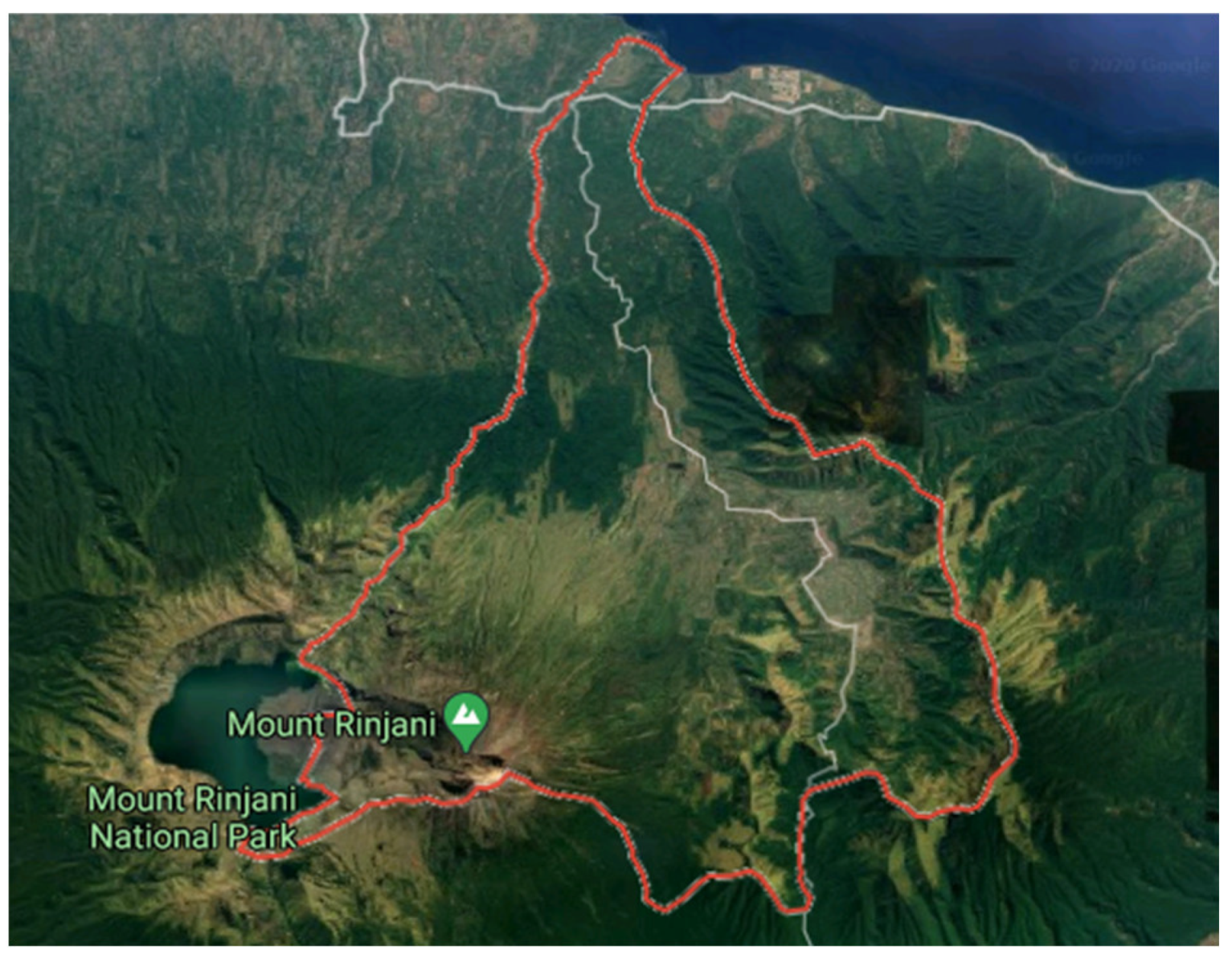
The satellite data used in this study were Sentinel-1A images for the Sembalun area of East Lombok, West Nusa Tenggara, Indonesia, which is located between 8°23 25.9″–8°22 06.4″ S and 116°31 32.9″–116°33 14.2″ on the slopes of Mount Rinjani (Figure 2). Sembalun is one of the 18 provinces which is included as the priority of the national garlic development program by the Ministry of Agriculture, Indonesia [19].
Sentinel-1A is a European radar imaging satellite that was launched in 2014 as part of the European Union’s Copernicus program. Sentinel-1A images provide the data for studies on the environment, security, economy, and global business. The Sentinel 1A images are also used for monitoring and mapping land cover. Sentinel-1 satellite images are derived from two satellites, Sentinel-1A and Sentinel-1B, whereby each of which is equipped with twin polar-orbiting satellites. Sentinel-1A has two polarizations (band), namely vertical transmit and vertical received (VV) and vertical transmit and horizontal received (VH). The image is represented in grayscale with single polarization (VV or VH). Meanwhile, each image in dual-polarization (VV, VH) is represented by a single RGB composite color, with the red channel (R) representing the first polarization, the green channel (G) representing the second polarization, and the blue channel (B) representing the average of the two polarization values [20]. The Sentinel-1A image specifications used in this study are listed in Table 1.

2.2. Research Steps

This study was conducted in four steps: (1) data partition, (2) classification modeling, (3) model evaluation, and (4) comparison of the classification models to other classifiers, as presented in Figure 3. In the k-NN implementation, the image data were divided into two partitions: 90% for Partition 1 and 10% for Partition 2, using 10-fold cross-validation. The k-fold cross-validation divides the sample data randomly into k-independent subsets of the same size. One subset is test data and the k-1 subset is the training data [21]. Partition 1 was separated into a training set (90%) and a validation set (10%) using 10-fold cross-validation. The training set was used to develop the model. Partition 2 was used as a testing set to test the model. The validation set was utilized for hyperparameter tuning. The classification model was evaluated in the testing stage. Hyperparameter tuning of k-NN was performed during the validation stage. The VH and VV bands were the band types used in the classification using the k-NN and MLC methods.
The classification models were created in three scenarios of bands referred to in [22]. These band scenarios are provided in Table 2. The study presented in [22] reveals that the more variables used, the higher the accuracy of the models produced. Hyperparameter tuning was conducted in k-NN classification to determine the optimum parameters of the k-NN method. The optimum hyperparameter increases accuracy and reduces losses. The GridSearchCV library was used for hyperparameter tuning to obtain the optimal hyperparameter values of a model. GridSearchCV is a function in Scikit-learn, a machine learning library for the Python programming language. This method works by calculating and assessing all possible parameters to obtain the best parameters for the highest accuracy of the model [23]. This study used GridSearchCV because this method evaluates and validates each hyperparameter combination automatically to produce a model with the best performance. When each hyperparameter combination is evaluated, GridSearchCV provides all possible classification models and selects the best model for prediction.
The implementation of the k-NN method on the dataset utilized the KNeighborClassifiers library in Python programming language [24]. The implementation of the MLC method used the rasclass library that is available in the R programming language. The classification model of garlic and non-garlic field identification was evaluated using the confusion matrix, as presented in Table 3. Accuracy, precision, and recall were calculated to evaluate the model’s performance. In addition, the run time analysis of the k-NN and MLC algorithms was used to assess the efficiency of the algorithms.
Accuracy and random accuracy were derived from the confusion matrix [25] as follows:
Accuracy = TP + TN TP + TN + FP + FN × 100 %
Random   Accuracy = ( TN + FP ) × ( TN + FN ) × ( FN + TP ) × ( FP + TP ) ( TP + TN + FP + FN ) × ( TP + TN + FP + FN )
Kappa finds the truth between the predicted and actual class. The equation of the kappa is as follows [25]:
Kappa =   Overall   Accuracy   Random   Accuracy   1   Random   Accuracy
Accuracy is also needed from samples labeled according to their class. Therefore, precision was calculated. Meanwhile, recall was used to measure the number of predicted objects that were truly relevant to the test data. The precision and recall equations were as follows:
Precision = TP TP + FP × 100 %
Recall = TP TP + FN × 100 %  

2.3. Data Preprocessing

The Sentinel-1A satellite images were obtained from Copernicus Open Access Hub ESA for July 2019 and November 2019 [26]. The type of Sentinel-1A image used was ground range detection (GRD) with a resolution of 20 × 5 m and a pixel size of 10 × 10 m. The image preprocessing was conducted using The Sentinel Application Platform (SNAP) [27]. SNAP was utilized to perform the following steps: apply orbit file, calibration, speckle filtering, terrain correction, and linear to dB conversion [28]. The feature Apply Orbit File is available in SNAP, which automatically downloads and updates the orbit condition for each SAR image. This feature accurately provides data on the position and speed of the satellite. In the calibration step, the digital number (DN) is calibrated to be backscatter in the form of sigmaθ that will be used for quantitative identification of the images. Speckle filtering is a procedure to improve image quality by reducing speckles. The objective of terrain correction is to compensate for geometric distortions so that the geometric representation will be as close as possible to the real image. Linear to dB is a step to convert the backscatter coefficient to decibels (dB) using the logistic transformation.
The preprocessed image was then clipped to capture the relevant research area, which was between 8°23 25.9″ and 8°22 06.4″ S and 116°31 32.9″ and 116°33 14.2″ T. The VV and VH band values were then extracted from 16,800 pixels, with 8400 pixels classified as garlic classes and 8400 pixels classified as non-garlic classes. The class labeling was performed based on field observation. The image from July represents an area that has just been planted with garlic, while the image from November represents an area that was in the harvest phase.
The dataset was divided into two parts based on the condition and information as to when garlic was planted and harvested. Dataset A contains data derived from images taken at the start of garlic planting and harvesting on 13 July 2019 and 10 November 2019, respectively. Dataset B was extracted from the image at the end of the garlic planting and the end of the garlic harvest on 25 July 2019 and 22 November 2019, respectively. Each dataset comprises 10% of 84,000 pixels, which is 8400 pixels. Each pixel has eight attributes, i.e., date, X, Y, longitude, latitude, VH band, VV band, and class. Table 4 shows that each dataset contains 4200 pixels of garlic samples and 4200 pixels of non-garlic samples. The holdout method was then used to divide each dataset into two parts: (1) 90% was used for training data (7560 pixels) and 10% was used for test data (840 pixels). Furthermore, the sample images with predetermined classes were converted to the relation format as the input of k-NN and MLC algorithms.
Table 5 and Table 6 show the data characteristics of the training set for each class. The training data consisting of VV and VH bands in the garlic class are close to a perfect normal distribution, as presented in Table 5 and Table 6. However, some data in the non-garlic class are laid beyond the bounds of normal distribution because the data variance was higher than in the garlic class. In addition, the mean, variance, and covariance values were used in the training stage to build a classification model. The prediction of each class will be based on the model obtained from the training stage.
In the k-NN method, the training and validation data were distributed using the 10-fold cross-validation approach in the GridSearchCV package of Scikit-Learn. The distribution of training data and test data was carried out using splitfraction in the ClassifyRasclass function. In the MLC method, the data were divided into two, i.e., 90% for training and 10% for testing. Each dataset was separated into three scenarios before going through the classification phase to obtain a band combination and compare the accuracy of the three scenarios.

2.4. K-Nearest Neighbor

The k-Nearest Neighbor (k-NN) method is a guided learning classification algorithm that discovers new patterns in data. The k-NN method works in two stages: the first is the determination of the nearest neighbors and the second is a calculation of the distance between classes using these neighbors [29]. By categorizing the test data into the class with the highest number of members based on the attributes and samples from the training data, the training data are projected into a multidimensional space represented as a feature of the data. The k-NN method calculates the distance between the new vector and all of the training data vectors; then, it selects a set of k neighbors with the shortest distance. Euclidean distance is commonly used in k-NN to calculate the distance between objects. The steps in k-NN are as follows:
  • Prepare input: training set, class of training data, testing set.
  • Calculate the distance between each object in the testing set to each object in the training set.
  • Determine k training objects that are nearest to the testing objects.
  • Define the label that frequently occurred.
  • Assign the testing object to the class with the highest frequency.
The k-NN approach has the benefit of being highly straightforward and easy to learn and use [29]. The k-NN method increases classification accuracy by using a noise reduction technique [29]. The k-NN method is a non-parametric approach with no data distribution assumption needed; thus, this approach is more flexible. However, the trial and error technique for parameter selection is a drawback of the k-NN method; therefore, more time is required for computation.
The implementation of the k-NN algorithm on the dataset utilizes the KNeighborClassifiers library in Python programming language. Two scenarios were executed in hyperparameter tuning in the k-NN algorithm: scenario A used 6 parameters and scenario B used 2 parameters. The hyperparameters in scenario A (6 parameters) were as follows [24]:
(1)
param_algorithm: algorithm used to compute the nearest neighbors;
(2)
param_leaf_size: leaf size passed to BallTree or KDTree;
(3)
param_metric: Metric for distance computation. The default is “minkowski”, which results in the standard Euclidean distance when power (p) = 2;
(4)
param_n_neighbor: number of neighbors;
(5)
param_p: power parameter for the Minkowski metric;
(6)
param_weights: weight function used in prediction.
The hyperparameters in scenario B (2 parameters) were as follows [24]:
(1)
param_n_neighbor: number of neighbors;
(2)
param_p: power parameter for the Minkowski metric.

2.5. Maximum Likelihood Classification

The maximum likelihood classification (MLC) method works based on Bayesian principles. The MLC method is a parametric algorithm that needs to estimate model parameters before making classification decisions [30]. The MLC is one of the most used methods to analyze satellite image data [31] which is typically used to compare and to calculate the average variance value between classes and existing bands. The classification process is based on the similar pixel value and recognition in the image and calculating the probability density for each class. The probability that a pixel with feature vector ω belongs to class i is defined by Bayes theory [32]:
P ( i | ω ) = P ( ω | i ) P ( i ) P ( ω )
where
P(ω|i) is the likelihood function;
P(i) is the probability of class i occurring in an image;
P(ω) is the probability that ω is observed.
P(ω) was calculated using the following formula [32]
P ( ω ) = i 1 M P ( ω | i ) P ( i )
where M is the number of classes. A pixel with feature vector ω is classified as class i if P ( i | ω ) > P ( j | ω ) for all i j [32].
The MLC method calculates the likelihood of a pixel value of a labeled object based on the statistical features of the training data. Training data contain numerous spectral classes which are used to estimate the probability of each class of pixel in the images by estimating the mean value vector and the matrix covariance. The training data are assumed to be regularly distributed, i.e., Gaussian, for each class in each band [33]. The result of classification is the class of objects with the highest probability.
The MLC method assumes that the training data are normally distributed, whereas the k-NN approach ignores this assumption. The parametric technique has the advantage that the time distribution can be simply approximated to execute each of the data, making the execution process faster. Meanwhile, the flaw is that if there are differences in the distribution to be considered, the parameters must be estimated and tested iteratively [34].

3. Results

3.1. Classification Using k-NN

This study evaluates the implementation of the k-NN method based on training time and accuracy. The selection of parameters in k-NN influences the training time during the model development. The parameters used in the classification process using the k-NN method are the number of neighbors (k) and the distance calculation method (p). Initially, the computation used a value of k neighbors from 1 to 30. Manhattan and Euclidean were selected as the distance calculation methods. A number of neighbors (k) above 30 was also randomly selected. However, the classification model accuracy decreased for the k value above 30. Therefore, the optimal range of k for hyperparameter tuning is between 1 and 30. Table 7 and Table 8 show a comparison of the training time in k-NN and the model’s accuracy. The experimental results in dataset A show that training with two parameters is much faster than training with six parameters. On average, the model’s accuracy with two parameters is higher than that of the model with six parameters. Therefore, a model with two parameters in Scenario 1 is selected as the best model from dataset A to classify garlic and non-garlic fields.
Table 7 shows the average accuracy of a k-NN model applied to dataset A. According to Table 7, the model’s accuracy of two parameters is slightly better than the accuracy of six parameters, which is improved from 74.37 % to 74.80 %. A significant difference was presented in computational time where the k-NN model of six parameters needed 4898.27 s to complete; however, the k-NN model of two parameters only needed 9.14 s to complete.
Table 8 shows the average accuracy of a k-NN model applied to dataset B. According to Table 8, the model’s accuracy of two parameters is slightly better than the accuracy of six parameters which is improved from 78.345 % to 78.65 %. A significant difference was presented in computational time where the k-NN model of six parameters needed 4811.67 s to complete; however, the k-NN model of two parameters only needed 9.06 s to complete.
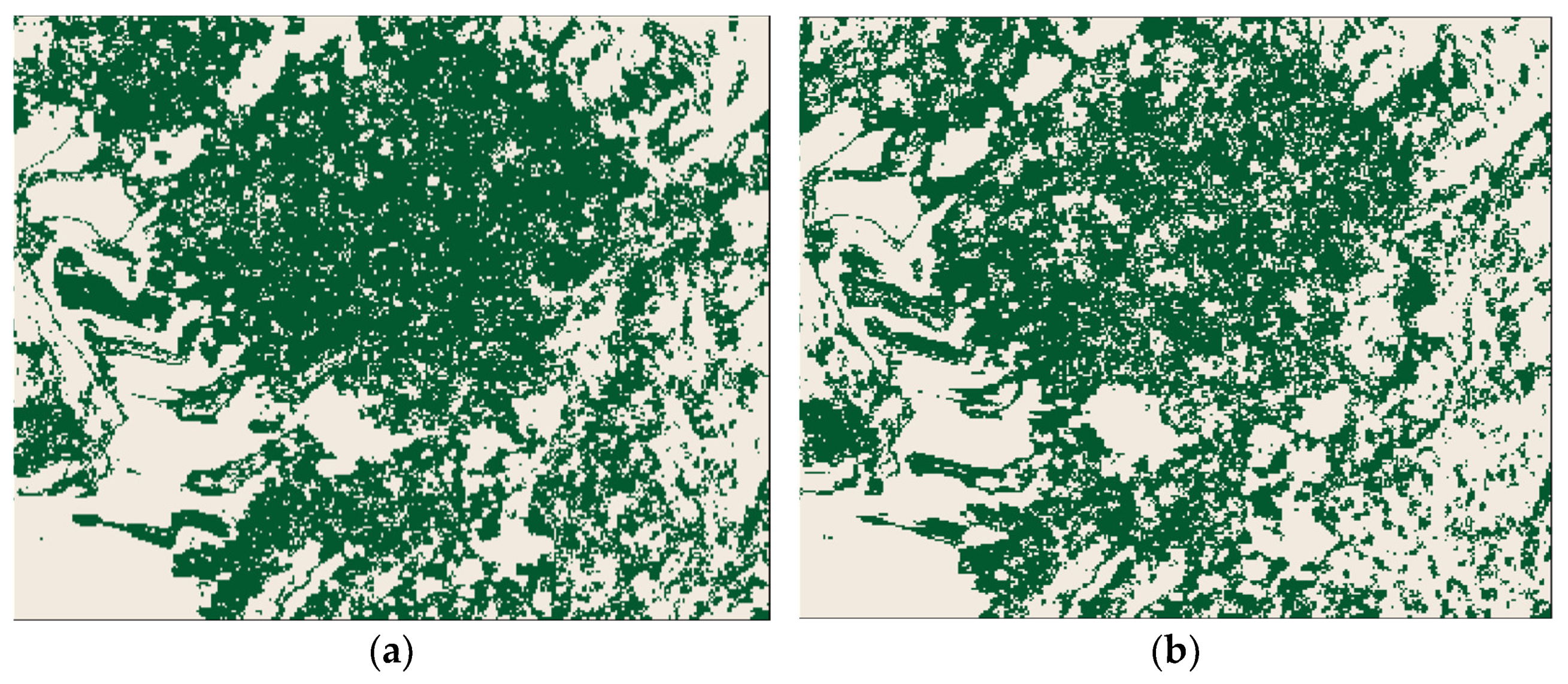
Table 9 shows the accuracy of classification models, the optimal parameters’ distance formula (p), and the number of neighbors in each dataset and scenario for the VH and VV bands’ combination. According to Table 9, additional bands in these scenarios do not increase the model accuracy significantly. As seen in dataset A, the growth is only by 0.1 % between Scenario 2 (VV, VH, and VV-VH) and Scenario 3 (VV, VH, VV-VH, (VV/VH), and (VV+VH)/2). Table 9 shows that Scenario 1 (VV and VH) has the highest overall accuracy of 75 % in dataset A. The distance calculation method (p) used is the Euclidean distance with a number of neighbors (n_neighbors) of 27. In dataset B, the model’s accuracy is 78.81 % with the Manhattan distance and a number of neighbors of 26. The study concludes that adding VH and VV bands’ combination does not increase the accuracy of garlic field classification models generated using the k-NN algorithm. The classification results of the garlic and non-garlic area using k-NN are visualized in Figure 4.
MLC is a parametric classification process where the probability distribution in each class is assumed to be normal. The maximum likelihood method in classifyRasclass, a function in the Rasclass package in the R programming language, was utilized to implement the MLC algorithm. An output in the raster grid was generated as part of the classification process, along with accuracy, the confusion matrix, and the kappa coefficient.
Table 10 shows the model’s accuracy generated using the MLC algorithm on each dataset and scenario for VH and VV bands’ combination. In Scenarios 2 and 3, datasets A and B were not able to produce the classification model and accuracy was denoted as Inf. This occurred because there was a determinant value of the variance–covariance matrix of the training data that was near zero, as presented in Table 11. The MLC algorithm formula in the denominator is the determinant of the variance–covariance matrix, resulting in an infinite. Thus, Scenario 1 has the highest overall accuracy in datasets A and B, with 74.88 % and 76.31 %, respectively.

3.2. Evaluation of Classification Models

This study compares k-NN and MLC models for garlic field classification based on training time, accuracy, precision, recall, and kappa coefficient. The k-NN and MLC computation were conducted using an Intel Core I i3-6006U PC with 4 GB of RAM. Table 12 compares the training time and accuracy achieved by the k-NN and MLC classification models. The best model using dataset B in Scenario 1 takes 0.8 s to train the training data using the MLC method. On the other hand, the overall training time for the classification model using the k-NN method is roughly 8.75 s slower but the model has better accuracy than MLC. Based on this result, it can be concluded that modeling using the k-NN method improves accuracy, while the MLC approach is efficient for garlic field classification. This is consistent with the claim that the MLC method is a parametric algorithm with benefits over non-parametric algorithms such as the k-NN method in terms of training time. The k-NN outperforms the MLC in terms of accuracy, where the k-NN model’s accuracy is 2.50% higher than the classifier from MLC, as presented in Table 12. When the assumption of normality datasets is known, the MLC is a good option, especially in terms of efficiency. K-NN has the benefit of generating classification models without knowing the assumption of normality datasets.
The garlic field classification models were evaluated using the accuracy, precision testing, recall, and kappa coefficient, as depicted in the confusion matrix presented in Table 13 and Table 14. According to the result of the k-NN and MLC classifier, the number of true positive and true negative objects in dataset B is higher than in dataset A.
In addition, according to the confusion matrix presented in Table 13 and Table 14, both k-NN and MLC classifiers do not work well on the objects with the labeled non-garlic field. In the k-NN model, about 35.48% of objects of the non-garlic field are classified as garlic fields in dataset A. In dataset B, approximately 31.43% of non-garlic objects are classified as garlic fields. Similarly to results in MLC, the number of non-garlic field objects incorrectly classified as garlic fields is about 43.65% in dataset A and 38.22% in dataset B. Thus, dataset B produces the best garlic field classification model in all scenarios of VH and VV bands’ combination. Dataset B performs better because there were variations in the planting period and garlic age.
The kappa, precision, and recall of the classification models are presented in Table 15, Table 16 and Table 17, respectively. The kappa values of k-NN and MLC classifiers range from 0.48 to 0.58, meaning that the models are imperfect in classifying garlic and non-garlic fields. The precision of the garlic field class is lower than for the non-garlic class. MLC and k-NN classifiers have a lower precision of garlic field than the non-garlic class because the number of false positive (FP) objects is higher than false negative (FN) objects. An FN indicates the number of garlic fields that the model incorrectly classifies as the non-garlic field. An FP represents the number of non-garlic fields that are correctly classified by the classifier as being garlic fields. To achieve a higher success rate in identifying the garlic fields, the FN value should be as low as possible to obtain a high recall. The recall of garlic classes in dataset B is 89% and 92%, respectively, resulting from k-NN and MLC, which is higher than in dataset A.
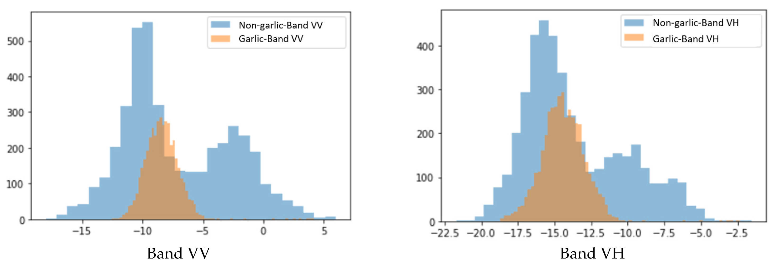
According to the precision, more than 80% of non-garlic fields are predicted as being non-garlic fields in both dataset A and dataset B, as presented in Table 16 and Table 17. The distribution of features VV and VH in Sentinel-1A is presented in Figure 5. The band VV and VH of garlic objects are overlapped with the non-garlic objects, as presented in Figure 5. More band combinations of VV and VH can be considered to separate garlic objects’ band distribution from non-garlic objects. Therefore, the number of incorrectly classified objects will decrease.

4. Discussion

This section discusses garlic field classification models generated using the k-NN and MLC models compared to the models from other machine learning algorithms developed in previous studies [8,9,10]. Table 18 provides the best models from the k-NN algorithm and MLC compared to the classifiers developed in previous studies. The classification model using the k-NN algorithm is better than the decision tree (DT) model [9] with an increase in accuracy of 0.36%, support vector machine (SVM) [8] with an increase in accuracy of 2.03%, and random forest (RF) [10] with an increase in accuracy of 0.36%. The conventional machine learning algorithms were implemented on Sentinel-1A satellite images [9,10]. DT, SVM, k-NN, and RF work on the pixel-based datasets with vertical–vertical (VV) and vertical–horizontal (VH) bands. The accuracy of classification models ranges from 76.78% to 78.81%. MLC produces the model with the lowest accuracy among the classification algorithms applied to garlic datasets. In addition to conventional machine learning algorithms, the previous study applied the convolutional neural network (CNN) to the Sentinel-1A satellite images. The CNN works on image-based classification in identifying garlic and non-garlic fields. The classification model has an accuracy of 86.36% [35] which is much higher than the accuracy of classifiers generated from pixel-based datasets. According to the results of previous studies, it can be summarized that the machine learning algorithms are more accurate in garlic field classification using Sentinel-1A satellite images than the statistical method. This is because the statistical method requires a normal data distribution assumption.

5. Conclusions

The classification of Sentinel-1A satellite images in the garlic field was successfully applied to two different datasets using the k-NN and MLC methods. The k-NN classification result is slightly better than other classification methods with the highest accuracy of 78.81%. The k-NN computation, especially with regard to the training time, is faster than other comparable methods, i.e., only 10 s. The best accuracy achieved from the classification results using the MLC is 76.31%, with a training time of 0.8 s. Both the k-NN and MLC models have limitations in classifying garlic objects because the VV and VH band distribution was not separated well among garlic and non-garlic objects. This study concludes that the machine learning approach is more suitable for pixel-based classification for garlic field identification using Sentinel-1A satellite images than the statistical method. The dataset’s quality is an issue to be solved in future work. The values of bands VV and VH are overlapped on the pixel with the garlic and non-garlic classes, so the number of misclassified pixels is high. Collecting new Sentinel-1A satellite images in different periods of garlic planting is required in following work to identify garlic and non-garlic objects clearly. The future study will improve the dataset quality to increase the model’s accuracy. The improvement will be performed in future works by considering more band combinations of VV and VH and the use of Sentinel 2-A with more bands than Sentinel-1A.

Author Contributions

Conceptualization, I.S.S., I.A.R., M.A.A. and S.S.; methodology, I.S.S., I.A.R. and M.A.A.; software, I.A.R. and M.A.A.; validation, M.A.A., W.C. and A.A.; formal analysis, I.S.S.; investigation, M.A.A., W.C. and A.A.; resources, M.A.A.; data curation, I.A.R. and M.A.A.; writing—original draft preparation, I.S.S., I.A.R. and A.A.; writing—review and editing, I.S.S. and W.C.; visualization, I.A.R. and A.A.; supervision, I.S.S. and M.A.A.; project administration, M.A.A., A.A. and S.S.; funding acquisition, I.S.S. and W.C. All authors have read and agreed to the published version of the manuscript.

Funding

This research was funded by IPB University under Program for Institutional Agromaritim (Research No. 7823/IT3.L1/PT.01.03/P/B/2021). The third author acknowledge the Polish National Agency for Academic Exchange (NAWA) No. BPN/ULM/2022/1/00139/U/00001 for partial financial support.

Data Availability Statement

We obtained the Sentinel-1A satellite imagery from Copernicus Open Access Hub, URL: https://scihub.copernicus.eu/dhus/ (accessed on 7 March 2023).

Acknowledgments

The authors would like to thank the European Space Agency for providing the Sentinel-1A satellite imagery and the tool for preprocessing the Sentinel-1A images.

Conflicts of Interest

The authors declare no conflict of interest.

References

  1. Statistics Indonesia and Directorate General of Horticulture. Garlic Productivity by Province, 2015–2019 (In Bahasa). Statistics Indonesia and Directorate General of Horticulture. Available online: https://www.pertanian.go.id/home/index.php?show=repo&fileNum=339 (accessed on 28 August 2022).
  2. Ministry of Agriculture Indonesia. Regulation of the Minister of Agriculture Indonesia Number 38 Year 2017 Concerning Recommendations for the Import of Horticultural Products. Ministry of Agriculture Indonesia. Available online: https://peraturan.bpk.go.id/Home/Download/153591/PermentanNomor38Tahun2017.pdf (accessed on 23 September 2022).
  3. Zulkarnain. Tropical Vegetable Cultivation; Bumi Aksara: Jakarta, Indonesia, 2013. (In Bahasa) [Google Scholar]
  4. Statistics Indonesia. Production of Vegetable Plants 2012 (In Bahasa). Statistics Indonesia. Available online: https://www.bps.go.id/indicator/55/61/10/produksi-tanaman-sayuran.html (accessed on 12 December 2022).
  5. Mayanda, D.P.; Adi, I.G.P.R.; Kusmiyarti, T.B. Evaluation of Land Suitability of Horticultural Crops in Sembalun Sub-district, East Lombok Regency, Indonesia. IOP Conf. Ser. Earth Environ. Sci. 2019, 313, 012018. [Google Scholar] [CrossRef] [Green Version]
  6. Muslim, R.Q.; Mulyani, A. Land characteristics and suitability for development of garlic in East Lombok Regency, West Nusa Tenggara Province. IOP Conf. Ser. Earth Environ. Sci. 2019, 393, 012079. [Google Scholar] [CrossRef]
  7. Mahmudah, N.; June, T. Impron Adaptive Garlic Farming on Climate Change and Variability in Lombok. Agromet 2021, 35, 116–124. [Google Scholar] [CrossRef]
  8. Agmalaro, M.A.; Sitanggang, I.S.; Waskito, M.L. Sentinel 1 Classification for Garlic Land Identification using Support Vector Machine. In Proceedings of the 2021 9th International Conference on Information and Communication Technology (ICoICT), Yogyakarta, Indonesia, 3–5 August 2021; pp. 440–444. [Google Scholar] [CrossRef]
  9. Komaraasih, R.I.; Sitanggang, I.S.; Agmalaro, M.A. Sentinel-1A Image Classification for Identification of Garlic Plants using a Decision Tree Algorithm. In Proceedings of the 2020 International Conference on Computer Science and Its Application in Agriculture (ICOSICA), Bogor, Indonesia, 16–17 September 2020; pp. 1–6. [Google Scholar] [CrossRef]
  10. Sitanggang, I.S.; Agmalaro, M.A.; D’Alene, A.A.C.; Annisa. Ensemble Learning on Sentinel-1A Imagery for Garlic Field Classification. In Proceedings of the 2022 International Conference of Informatics, Multimedia, Cyber, and Information System (ICIMCIS), Jakarta, Indonesia, 16–17 November 2022. [Google Scholar]
  11. Chai, Z.; Zhang, H.; Xu, X.; Zhang, L. Garlic Mapping for Sentinel-2 Time-Series Data Using a Random Forest Classifier. In Proceedings of the IGARSS 2019—2019 IEEE International Geoscience and Remote Sensing Symposium, Yokohama, Japan, 28 July–2 August 2019; pp. 7224–7227. [Google Scholar] [CrossRef]
  12. Wu, S.; Lu, H.; Guan, H.; Chen, Y.; Qiao, D.; Deng, L. Optimal Bands Combination Selection for Extracting Garlic Planting Area with Multi-Temporal Sentinel-2 Imagery. Sensors 2021, 21, 5556. [Google Scholar] [CrossRef] [PubMed]
  13. Maharani, E.; Sitanggang, I.S.; Agmalaro, M.A. Garlic Growth Phase Classification using Support Vector Machine and Sentinel-2A Imagery. In Proceedings of the 2022 6th International Conference on Informatics and Computational Sciences (ICICoS), Semarang, Indonesia, 28–29 September 2022; pp. 72–77. [Google Scholar] [CrossRef]
  14. Tian, H.; Pei, J.; Huang, J.; Li, X.; Wang, J.; Zhou, B.; Qin, Y.; Wang, L. Garlic and Winter Wheat Identification Based on Active and Passive Satellite Imagery and the Google Earth Engine in Northern China. Remote Sens. 2020, 12, 3539. [Google Scholar] [CrossRef]
  15. Nurkholis, A.; Sitanggang, I.S.; Annisa, A.; Sobir, S. Spatial decision tree model for garlic land suitability evaluation. IAES Int. J. Artif. Intell. IJ-AI 2021, 10, 666–675. [Google Scholar] [CrossRef]
  16. Felegari, S.; Sharifi, A.; Moravej, K.; Amin, M.; Golchin, A.; Muzirafuti, A.; Tariq, A.; Zhao, N. Integration of Sentinel 1 and Sentinel 2 Satellite Images for Crop Mapping. Appl. Sci. 2021, 11, 10104. [Google Scholar] [CrossRef]
  17. Moola, W.S.; Bijker, W.; Belgiu, M.; Li, M. Vegetable mapping using fuzzy classification of Dynamic Time Warping distances from time series of Sentinel-1A images. Int. J. Appl. Earth Obs. Geoinf. 2021, 102, 102405. [Google Scholar] [CrossRef]
  18. The European Space Agency. Sentinel-1 SAR Overview: Geophysical Measurements. The European Space Agency. Available online: https://sentinels.copernicus.eu/web/sentinel/user-guides/sentinel-1-sar/product-overview/geophysical-measurements (accessed on 28 December 2022).
  19. Ministry of Agriculture. Decree of the Minister of Agriculture No. 472/Kpts/RC.040/6/2018 Concerning the Location of National Agricultural Areas. Ministry of Agriculture. 2018. Available online: https://peraturan.bpk.go.id/Home/Details/162567/kepmentan-no-472kptsrc04062018-tahun-2018 (accessed on 26 December 2022).
  20. The European Space Agency. User Guides Sentinel-1 SAR: Acquisition Modes. The European Space Agency. Available online: https://sentinels.copernicus.eu/web/sentinel/user-guides/sentinel-1-sar/acquisition-modes (accessed on 28 December 2022).
  21. Kohavi, R. A study of cross-validation and bootstrap for accuracy estimation and model selection. Presented at the IJCAI’95. In Proceedings of the 14th International Joint Conference on Artificial Intelligence, Montreal, QC, Canada, 20–25 August 1995; Volume 2, pp. 1137–1143. [Google Scholar]
  22. Abdikan, S.; Sanli, F.B.; Ustuner, M.; Calò, F. Land Cover Mapping using Sentinel-1 SAR Data. Int. Arch. Photogramm. Remote Sens. Spat. Inf. Sci. 2016, XLI-B7, 757–761. [Google Scholar] [CrossRef] [Green Version]
  23. Siji, G.C.G.; Sumathi, B. Grid Search Tuning of Hyperparameters in Random Forest Classifier for Customer Feedback Sentiment Prediction. Int. J. Adv. Comput. Sci. Appl. 2020, 11, 174. [Google Scholar] [CrossRef]
  24. Scikit-learn Developers. Sklearn.Neighbors. KNeighborsClassifier. Scikit-Learn Developers. 2022. Available online: https://scikit-learn.org/stable/modules/generated/sklearn.neighbors.KNeighborsClassifier.html (accessed on 28 December 2022).
  25. Witten, I.H.; Frank, E.; Hall, M.A. Data Mining: Practical Machine Learning Tools and Techniques, 3rd ed.; Elsevier: Burlington, NJ, USA, 2011; ISBN 978-0-12-374856-0. [Google Scholar] [CrossRef] [Green Version]
  26. ESA Copernicus. Copernicus Open Access Hub. Available online: https://scihub.copernicus.eu/dhus/ (accessed on 7 November 2020).
  27. SNAP—ESA Science Toolbox Exploitation Platrom (STEP). European Space Agency. 2017. Available online: http://step.esa.int/main/toolboxes/snap/ (accessed on 7 November 2020).
  28. Filipponi, F. Sentinel-1 GRD Preprocessing Workflow. Proceedings 2019, 18, 11. [Google Scholar] [CrossRef] [Green Version]
  29. Cunningham, P.; Delany, S.J. k-Nearest Neighbour Classifiers—A Tutorial. ACM Comput. Surv. 2021, 54, 1–25. [Google Scholar] [CrossRef]
  30. Zhang, Y.; Ren, J.; Jiang, J. Combining MLC and SVM Classifiers for Learning Based Decision Making: Analysis and Evaluations. Comput. Intell. Neurosci. 2015, 2015, 423581. [Google Scholar] [CrossRef] [PubMed]
  31. Richards, J.A. Remote Sensing Digital Image Analysis; Springer: Berlin/Heidelberg, Germany, 2013. [Google Scholar] [CrossRef]
  32. Ahmad, A.; Quegan, S. Analysis of Maximum Likelihood Classification on Multispectral Data. Appl. Math. Sci. 2012, 6, 6425–6436. [Google Scholar]
  33. Jensen, J.R.; Lulla, K. Introductory Digital Image Processing: A Remote Sensing Perspective, 2nd ed.; Prentice Hall: Hoboken, NJ, USA, 1996. [Google Scholar]
  34. Worms, J.; Touati, S. Parametric and Non-Parametric Statistics for Program Performance Analysis and Comparison. Universite Nice Sophia Antipolis; Universite Versailles Saint Quentin en Yvelines; Laboratoire de Mathematiques de Versailles, Research Report. 2016. Available online: https://hal.inria.fr/hal-01286112v3/document (accessed on 7 November 2020).
  35. Komaraasih, R.I.; Sitanggang, I.S.; Annisa, A.; Agmalaro, M.A. Sentinel-1A image classification for identification of garlic plants using decision tree and convolutional neural network. IAES Int. J. Artif. Intell. IJ-AI 2022, 11, 1323–1332. [Google Scholar] [CrossRef]
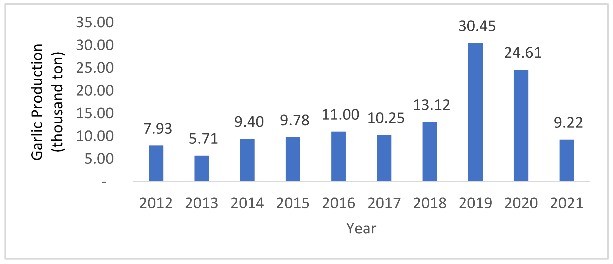
Figure 1. Garlic production (thousand tons) in West Nusa Tenggara, Indonesia, in 2012–2021 [4].
Agriengineering 05 00040 g001
Figure 2. Satellite image of Sembalun District, East Lombok, Indonesia.
Agriengineering 05 00040 g002
Figure 3. Steps in garlic field classification.
Agriengineering 05 00040 g003
Figure 4. Classification results of garlic and non-garlic areas using k-NN on (a) 13 July 2019 and (b) 10 November 2019. Note: green indicates the garlic field, and white indicates the non-garlic field.
Agriengineering 05 00040 g004
Figure 5. Histograms of the two classes in the VV and VH bands (decibel (dB)) of Sentinel-1A images [35].
Agriengineering 05 00040 g005
Table 1. Sentinel-1A image specifications.
AttributeSpecification
Acquisition time July and November 2019
Acquisition orbitAscending
Imaging modeInterferometry wide swath (IW)
Imaging frequencyTopsar Band-C center frequency 5.405Ghz
PolarizationVV-VH
Data product20–45°
Resolution modeLevel-1 GRD
Table 2. Scenario for VH and VV bands’ combination.
ScenarioDescription
1VV, VH
2VV, VH, VV-VH
3VV, VH, VV-VH, (VV/VH), (VV+VH)/2
Table 3. Confusion matrix [25].
Predicted Class
YesNo
Actual classYesTrue positive (TP)False negative (FN)
NoFalse positive (FP)True negative (TN)
Table 4. Image composition for each dataset.
DatasetGarlic Class SampleNon-Garlic Class Sample
A4200-pixel of the image on 13 July 20194200-pixel of the image on 10 November 2019
B4200-pixel of the image on 25 July 20194200-pixel of the image on 22 November 2019
Table 5. Characteristics of bands VH and VV in dataset A.
ClassBandMeanVarianceCovariance
GarlicVV−8.37741.59480.4375
VH−14.30802.0871
Non-garlicVV−5.409219.035213.6106
VH−12.229813.6658
Table 6. Characteristics of bands VH and VV in dataset B.
ClassBandMeanVarianceCovariance
GarlicVV−8.57711.97910.5216
VH−14.45571.9043
Non-garlicVV−5.719819.830014.8938
VH−12.637015.1894
Table 7. Model’s accuracy and training time of k-NN on dataset A.
ScenarioSix ParametersTwo Parameters
Time (s)Accuracy (%)Time (s)Accuracy (%)
14624.2775.009.6075.00
24906.2773.338.6374.64
35164.2574.769.1974.76
Average4898.2774.379.1474.80
Table 8. Model’s accuracy and training time of k-NN on dataset B.
ScenarioSix ParametersTwo Parameters
Time (s)Accuracy (%)Time (s)Accuracy (%)
14478.1578.819.5578.81
24760.4378.458.5378.45
35196.4278.109.1178.69
Average4811.6778.459.0678.65
Table 9. Model’s accuracy and the optimal hyperparameters in k-NN.
Dataset ADataset B
Scenariopn_neighborsAccuracy (%)pn_neighborsAccuracy (%)
12 (Euclidean) 2775.001 (Manhattan)2678.81
21 (Manhattan)2774.642 (Euclidean) 2978.45
31 (Manhattan)2974.762 (Euclidean)2878.69
Table 10. Classification model accuracy for datasets A and B.
Dataset Accuracy (%)
Scenario 1Scenario 2Scenario 3
A74.88InfInf
B76.31InfInf
Table 11. Determinant of the variance-covariance matrix for datasets A and B.
Garlic FieldNon-Garlic Field
Dataset ADataset BDataset ADataset B
DeterminantScenario 13.143.4975.0279.45
Scenario 25.57 × 10−156.21 × 10−156.66 × 10⁻¹⁴−6.35 × 10⁻¹³
Scenario 32.95 × 10−343.01 × 10−341.08 × 10−290
Table 12. Comparison of training time and model’s accuracy generated using the k-NN and MLC methods.
MethodTime (s)Accuracy (%)
k-nearest neighbor9.5578.81
Maximum likelihood classification0.876.31
Table 13. Confusion matrix of classification model generated using the k-NN method.
Actual ClassPrediction Class
Dataset ADataset B
Garlic FieldNon-Garlic FieldGarlic FieldNon-Garlic Field
Garlic field3596137446
Non-garlic field149271132288
Table 14. Confusion matrix of classification model generated using the MLC method.
Actual ClassPrediction Class
Dataset ADataset B
Garlic FieldNon-Garlic FieldGarlic FieldNon-Garlic Field
Garlic field4073937132
Non-garlic field172222167270
Table 15. Kappa value of classification models generated using the k-NN and MLC methods.
KappaAccuracy (%)
k-NN AlgorithmMLC Algorithmk-NN AlgorithmMLC Algorithm
Dataset A0.500.4875.0074.88
Dataset B0.580.5378.8176.31
Table 16. Precision and recall of garlic classification model generated using the k-NN method.
Dataset ADataset B
Precision (%)Recall (%)Precision (%)Recall (%)
Garlic field71857489
Non-garlic field82658669
Average77758079
Table 17. Precision and recall of garlic classification model generated using the MLC method.
Dataset ADataset B
Precision (%)Recall (%)Precision (%)Recall (%)
Garlic field70916992
Non-garlic field85568962
Average78747977
Table 18. Comparison of the model’s accuracy in this study with previous studies.
AlgorithmAccuracy (%)
Decision tree [9]78.45
Support vector machine [8]76.78
Random forest [10]78.45
k-nearest neighbor78.81
Maximum likelihood classification76.31
Convolutional neural network [35]86.36
Disclaimer/Publisher’s Note: The statements, opinions and data contained in all publications are solely those of the individual author(s) and contributor(s) and not of MDPI and/or the editor(s). MDPI and/or the editor(s) disclaim responsibility for any injury to people or property resulting from any ideas, methods, instructions or products referred to in the content.