A Self-Adaptive Framework for Sustainable Smart Cities

Highlights

What are the main findings?

• A holistic approach to the management of smart city infrastructure (social, economic, environmental) sustainability.
• An adaptive, intelligent framework to enforce overall urban sustainability through smart city infrastructure sustainability.

What are the implications of the main findings?

• The proposed solution and case study provide a methodology and a tool for urban planners to transition from static, siloed smart city deployments to adaptive and sustainable ones.
• The presented technique and process meet fine-grained urban sustainability requirements by acting on infrastructural metrics to address the operational targets of UN Sustainable Development Goal 11.

Abstract

The transition from traditional siloed to intelligent cities allows for the deployment and management of information and communication technologies in the urban context to be driven by holistic sustainability requirements rather than technical ones such as feasibility and fragmented, siloed operational patterns. This work proposes a multi-dimensional decision-making framework to manage a smart city as an urban cognitive Cyber–Physical System (CPS) across environmental, economic, and social sustainability pillars, metrics and their trade-offs. A methodology based on Deep Reinforcement Learning (DRL), specifically adopting Deep Q-Networks (DQNs), is proposed to represent and assess sustainability pillar dependencies and their interplay. A case study on Low-Power Wide-Area Network planning, deployment and management in a Sicilian municipality has been developed to demonstrate the effectiveness of the proposed approach in dealing with the dynamics and non-linear dependencies of the sustainability pillars.

1. Introduction

The modern urban environment is conceptualized as a highly complex and dynamic ecosystem where the integration of physical infrastructures and computational elements is essential for maintaining a high quality of life [1,2]. In this context, municipalities face multi-dimensional, often conflicting challenges, including infrastructure degradation, inadequate public service provision, surging operational costs, and escalating environmental impacts. These compounding challenges are central to the 11th United Nations Sustainable Development Goal (SDG 11), which focuses on the creation of inclusive, safe, resilient, and sustainable cities and communities (Figure 1) [3].

Addressing these demands requires a fundamental paradigm shift from traditional smart cities to intelligent urban ecosystems within the Society 5.0 framework, placing humans at the center of decision processes [4]. While conventional smart city frameworks are typically restricted to passive data collection, localized monitoring, and siloed vertical configurations, intelligent cities operate as cognitive Cyber–Physical Systems (CPSs). Supported by robust infrastructures, institutional quality, and inclusive policies [5], these systems enable autonomous, dynamic, and closed-loop adaptation to achieve multi-objective sustainability requirements. In this scenario, social sustainability ($P_s$) is crucial for livable communities focused on human well-being [6,7] through a deep integration of the environment, technology, and citizens [8].

Despite the potential of cognitive CPSs, the long-term sustainability of the underlying Information and Communication Technology (ICT) infrastructure remains a critical bottleneck. Current deployments suffer from a static bias, where edge nodes and networks are specifically engineered for fixed vertical configurations. Their parameters remain unchanged regardless of contextual fluctuations, leading to low resource reuse and high vulnerability to unpredictable demand variations. Managing these smart device fleets requires a balance between policy and technology. While engineers optimize technical metrics, municipal policymakers prioritize safety, equity, and the SDGs.

1.1. Why: The Environmental and Operational Conflict

The core challenge for intelligent cities is to contemporarily manage local resource constraints (economic sustainability, $P_c$) and preserve natural urban ecosystems (environmental sustainability, $P_e$). To bridge this gap, urban infrastructures have shifted toward the Artificial Intelligence of Things (AIoT) [9] and fully autonomous networks [10]. A fundamental milestone in this evolution is the synergy between AIoT and digital twins (DTs), acting as a smart city “brain” for predictive planning and real-time environmental management [11].

However, while macro-scale studies evaluate environmental and economic trade-offs through aggregated top-down indicators [12,13], they lack bottom-up, real-time adaptation loops operating at the physical device layer. In such a volatile context, maintaining the precise balance between ecosystem conservation and local network infrastructure bounds remains an open challenge. Indeed, prior attempts to predict renewable energy or carbon footprints often show reduced accuracy under highly unstable conditions or rely strictly on simulation testbeds without rigorous field validation [14,15,16].

When edge policies are designed with a purely passive approach (e.g., a permanent low-power approach), they introduce a high risk of information loss due to server-side under-provisioning. For example, during high-traffic commuter hours, this communication gap triggers data blackouts that collapse top-level smart mobility applications, such as dynamic routing and parking optimization algorithms. Crucially, this results in a systematic underestimation of localized traffic and pollution levels, forcing vehicles into extended cruising loops that drastically inflate indirect pollution.

Conversely, highly responsive policies could severely stress the CPS. For example, although this alternative approach effectively absorbs traffic peaks and minimizes data drops, it traps network nodes into continuous maximum power dissipation even during low-activity hours, heavily impacting operational costs and the direct energy consumption of electronic devices.

1.2. What: The Multi-Dimensional Decoupling Approach

To resolve these non-linear dependencies, this work introduces an adaptive urban framework designed to overcome limitations due to macro-scale top-down aggregated simulators or rigid threshold-based heuristics. The framework successfully models and resolves the non-linear dependencies and operational trade-offs among environmental, economic, and social sustainability pillars, establishing a formal link, as summarized in

Table 1. Comprehensive mapping of the proposed framework to SDG 11 targets and implementation strategies.

Sustainability Pillar	SDG 11 Targets	Framework Contribution
Environmental ($P_e$)	11.6 Environment	Minimizes the urban carbon footprint by mitigating traffic-related emissions. It dynamically regulates district resources to counter pollution peaks, ensuring a synergy between energy conservation and the overall environmental quality of the city area.
Economic ($P_c$)	11.4, 11.5 Heritage, Resilience	Minimizes economic impact by deploying resilient monitoring networks for urban heritage and early-warning systems. It reduces financial losses and recovery costs from environmental disasters through proactive infrastructure management and efficient resource allocation.
Social ($P_s$)	11.1, 11.2, 11.7 Housing, Transport, Public Spaces	Guarantees the necessary operational performance for smart mobility services, preventing service disruptions in urban transport infrastructures. It ensures that public transit and pedestrian spaces remain safe, accessible, and inclusive by maintaining reliable connectivity and real-time data flow.
Integrated ($P_e,P_c,P_s$)	11.3 Urbanization	Orchestrates participatory settlement planning by adapting to dynamic “bio-social” demands through multi-objective optimization.
	11.a Regional Planning	Supports strong links between urban and rural areas, overcoming silo patterns.
	11.b Integrated Policies	Internalizes multi-dimensional rewards to promote resource efficiency, climate change mitigation, and adaptive urban resilience.
	11.c Sustainable Building	Provides municipalities with a dynamic instrument for “adaptive” city planning, focusing on sustainable infrastructure and resilient buildings.

.

1.3. How: Edge-Constrained Cognitive Intelligence

Achieving this real-time, multi-objective synchronization exceeds the capabilities of classical computational methods or open-loop supervised models, which are structurally unfeasible for live parameter adjustments on resource-constrained hardware or heavily reliant on unavailable labeled data. To bridge this gap, an intelligent edge layer driven by Deep Reinforcement Learning (DRL), specifically Deep Q-Networks (DQNs), is deployed at each edge gateway to execute localized runtime inference.

The practical effectiveness and validation of this model are demonstrated through a concrete case study focusing on Low-Power Wide-Area Network (LPWAN) [17] infrastructures, utilizing Long-Range Wide-Area Network (LoRaWAN) specifications [18] deployed within a real municipal testbed.

The remainder of this work is organized as follows: Section 2 discusses materials and methods, presenting the proposed approach and sustainability metrics; Section 3 details the experimental case study; Section 4 analyzes the results of our investigation; and Section 5 concludes the work with future perspectives.

2. Materials and Methods

This section details the architectural layout, mathematical formalization, and algorithmic implementation of the proposed framework, alongside the state-of-the-art computational paradigm analysis that justifies the selection of our edge cognitive layer.

2.1. State-of-the-Art and Paradigm Comparison

Achieving real-time, closed-loop adaptivity across multi-dimensional urban requirements exceeds the capabilities of classical methods [19,20]. To map the state-of-the-art computational approaches within the smart city framework,

Table 2. Comparative assessment of Classical Methods (CMs), Supervised Learning (SL), and Reinforcement Learning (RL)/Deep RL (DRL) in the smart city scenario.

Feature	CMs (LP/Heuristics)	SL	RL / DRL
Logic	Rigid pre-defined rules; requires precise closed-form models.	Historical pattern matching; handles predictive urban tasks [21,22].	Goal-oriented optimization via active environmental feedback [23] and autonomous explore–exploit policies [24].
Limits	Incapable of adapting to dynamic contextual shifts.	Demands massive, perfectly labeled training datasets.	Asymmetrical computational workload between training and inference cycles [14,25].
Control	Open-loop execution.	Passive observation without active control loops.	Active closed-loop feedback and multi-agent distributed municipal coordination [26,27,28].
Target	Fixed static thresholds.	Replicates historical patterns and biases [29,30].	Dynamic Pareto balancing under multi-objective, non-linear physical infrastructure constraints [31,32].
Scaling	Non-scalable to decentralized networks.	Restricted to centralized data aggregation structures [33].	Leverages LLM feedback loops [34,35], DNN high-dimensional feature extraction [36], and federated wide-area learning [37].
Edge Deploy	Lightweight but inflexible.	Memory-intensive for continuous field deployment.	Lightweight localized inference; DQN architectures successfully break the urban “curse of dimensionality” [38,39,40,41].

provides a comprehensive comparative assessment of Classical Methods (CMs), Supervised Learning (SL), and Reinforcement Learning (RL)/Deep RL (DRL) configurations across core architectural features, scalability vectors, and design bottlenecks.

To contextualize these developments within specific state-of-the-art implementations,

Table 3. Strategic comparison of the proposed framework against recent state-of-the-art RL-based smart city approaches, categorized by methodological domain.

Methodological Domain	Key References	Core Urban Focus	Open Research Gap/Limitations	Sustainability Pillars
Urban Planning	Park et al. (2025) [41] Alharbi (2026) [42] Abu et al. (2025) [13]	Top-down multi-objective city planning, macro-indicator tracking, and policy validation via digital twins.	Operate primarily on high-level aggregated data; lack a bottom-up, dynamic adaptation mechanism at the physical infrastructure layer.	Economic Environmental
Smart Energy & Grid Demand Response	Sajid et al. (2026) [43] Michailidis et al. (2025) [44] Mai et al. (2024) [45] Shafiullah et al. (2026) [14]	Prosumer community management, fast-timescale residential load balancing, and renewable energy optimization.	Siloed applications restricted strictly to power grids and building facilities; do not scale to generalized municipal ICT constraints.	Economic Environmental
Urban Mobility & Logistics	Agarwal et al. (2021) [46] Kim & Chan (2025) [21] Fatorachian et al. (2025b) [30]	Autonomous driving policies, pedestrian road-crossing safety alerts, and IoT-driven predictive logistics.	Highly specific vertical applications; do not account for the structural energy and communication trade-offs of the underlying network.	Social Economic
Data Collection & Smart Sensing	Kim et al. (2023) [39] Zhang et al. (2018) [40] Bibri & Huang (2025) [11] Ficili et al. (2025) [32] Beguni et al. (2026) [37]	Energy harvesting in sensor nodes, unmanned vehicle data routing, federated demand prediction, and real-time AIoT city brain architectures.	Focus mostly on localized data-gathering efficiency or single technical metrics (e.g., node battery lifespan) without holistic optimization.	Environmental Economic
Proposed Framework	This Work	Balancing Resource Constraints and Responsive CPSs for Adaptive and Sustainable Smart Cities.	Introduces a bottom-up, adaptive DQN control loop that explicitly models and resolves the non-linear operational trade-offs among all three pillars.	Integrated (Environmental, Economic, Social)

maps the recent literature against our proposed framework, highlighting how this work fills the structural gap in physical network infrastructures.

Metaheuristics like Genetic Algorithms (GAs) or Particle Swarm Optimization (PSO) [41,47,48,49,50] are predominantly restricted to top-down, offline simulations or macro-indicator tracking. Because these population-based methods require iterative, multi-generation evaluations at runtime, they are structurally unfeasible for live parameter adjustment within resource-constrained edge gateways. On the other hand, while traditional tabular RL approaches [43] avoid this computational burden, they suffer from the “curse of dimensionality,” limiting their scope to low-dimensional, highly simplified urban domains.

To address the limitations of existing frameworks, the main contribution of this work is the proposal of a holistic, closed-loop approach to multi-dimensional urban sustainability, formalized through three interconnected pillars: environmental ($P_e$), economic ($P_c$), and social ($P_s$). Moving beyond traditional siloed patterns, the proposed methodology integrates a real-time, adaptive AI-driven model based on DRL and DQN. The DQN agent is specifically designed to resolve non-linear operational trade-offs among the metrics of the three sustainability pillars, optimizing infrastructure configurations in response to environmental and behavioral shifts.

A methodological and computational edge-constrained comparison of optimization patterns is reported in Table 4. It categorizes recent state-of-the-art implementations on resource-constrained edge hardware and highlights how this work differs from simple threshold-based rules, GA, Multi-Objective GA (MO-GA), PSO, Model Predictive Control (MPC), classical Q-Learning, and Proximal Policy Optimization (PPO)/Advantage Actor–Critic (A2C).

The recent literature demonstrates that while metaheuristics effectively optimize macro-scale urban domains, such as energy scheduling in smart grids [51,52] or congestion routing in intelligent transportation systems [53], their structural reliance on heavy global iterations confines their execution to centralized utility tiers or high-performance cloud frameworks, preventing real-time adaptive control at the localized, low-power network edge.

Table 4. Methodological and computational edge-constrained comparison of optimization patterns.

Method Class	Specific Method	Reference	Algorithmic Optimization Pattern	Reported Edge/Architectural Constraints
Heuristics	Threshold-based rules	Bruneel (2025) [54]	Trivial execution of static if–then–else logical conditional branches.	Fails under non-linear urban dynamics; zero multi-objective adaptability.
Metaheuristics	MO-GA	Hu et al. (2013) [51]	Multi-objective load balancing and demand-side management schedules.	High centralized computational overhead; non-real-time scaling.
	GA	Li et al. (2023) [47]	Latency-optimal scheduling for directed acyclic graph applications.	Reliant on task-offloading schemes to balance node capacity.
		Jyoti & Gokuldhev (2026) [49]	Probabilistic evolutionary search for task allocation routing.	Prohibitive convergence times (up to ∼10.8 s) under high iterations.
		Odeh et al. (2026) [53]	Congestion-aware vehicle routing and flow optimization loops.	Intended for cloud-enabled ITS frameworks; runtime delays on constrained nodes.
	GA/PSO	Molokomme et al. (2026) [48]	Iterative metaheuristic load balancing under heterogeneous task arrivals.	High local resource variability; requires emulated testing setups.
	Generic Metaheuristics	Mousavi-Ghasemlou et al. (2026) [52]	Sustainable energy deployment and macro resource distribution grids.	Restricted to centralized utility tiers; lacks low-power edge local autonomy.
Control Theory	MPC	Fryganiotis et al. (2025) [55]	Solves a complex, constrained multi-variable optimization problem online at each step.	Intolerable mathematical and processing overhead on low-power embedded CPUs.
Tabular RL	Q-Learning	Terven (2025) [19]	Direct memory lookup and cell-coordinate extraction from a fixed multi-dimensional array.	Memory saturation; exponential table explosion; unable to generalize to unseen states.
Actor–Critic RL	PPO/A2C	Terven (2025) [19], Plaat (2022) [20], Oh et al. (2025) [24], Hady et al. (2025) [27]	Dual-network inference tracking: concurrent execution of separate Actor and Critic layers.	Redundant memory footprint allocation; inflated localized inference latency for discrete actions.
Deep RL (DRL)	DQN	This Work	Asymmetric profile: offline training vs. online localized inference.	Bypasses iterative loops via deterministic forward pass to be deployed on edge gateways (case study in Section 3).

Table 4. Methodological and computational edge-constrained comparison of optimization patterns.

Method Class	Specific Method	Reference	Algorithmic Optimization Pattern	Reported Edge/Architectural Constraints
Heuristics	Threshold-based rules	Bruneel (2025) [54]	Trivial execution of static if–then–else logical conditional branches.	Fails under non-linear urban dynamics; zero multi-objective adaptability.
Metaheuristics	MO-GA	Hu et al. (2013) [51]	Multi-objective load balancing and demand-side management schedules.	High centralized computational overhead; non-real-time scaling.
	GA	Li et al. (2023) [47]	Latency-optimal scheduling for directed acyclic graph applications.	Reliant on task-offloading schemes to balance node capacity.
		Jyoti & Gokuldhev (2026) [49]	Probabilistic evolutionary search for task allocation routing.	Prohibitive convergence times (up to ∼10.8 s) under high iterations.
		Odeh et al. (2026) [53]	Congestion-aware vehicle routing and flow optimization loops.	Intended for cloud-enabled ITS frameworks; runtime delays on constrained nodes.
	GA/PSO	Molokomme et al. (2026) [48]	Iterative metaheuristic load balancing under heterogeneous task arrivals.	High local resource variability; requires emulated testing setups.
	Generic Metaheuristics	Mousavi-Ghasemlou et al. (2026) [52]	Sustainable energy deployment and macro resource distribution grids.	Restricted to centralized utility tiers; lacks low-power edge local autonomy.
Control Theory	MPC	Fryganiotis et al. (2025) [55]	Solves a complex, constrained multi-variable optimization problem online at each step.	Intolerable mathematical and processing overhead on low-power embedded CPUs.
Tabular RL	Q-Learning	Terven (2025) [19]	Direct memory lookup and cell-coordinate extraction from a fixed multi-dimensional array.	Memory saturation; exponential table explosion; unable to generalize to unseen states.
Actor–Critic RL	PPO/A2C	Terven (2025) [19], Plaat (2022) [20], Oh et al. (2025) [24], Hady et al. (2025) [27]	Dual-network inference tracking: concurrent execution of separate Actor and Critic layers.	Redundant memory footprint allocation; inflated localized inference latency for discrete actions.
Deep RL (DRL)	DQN	This Work	Asymmetric profile: offline training vs. online localized inference.	Bypasses iterative loops via deterministic forward pass to be deployed on edge gateways (case study in Section 3).

Although structural genetic approaches can optimize latency profiles for directed acyclic graphs, cooperative task-offloading mechanisms are implemented to manage the localized computing threshold of the node [47]. Executing GA/PSO within edge environments presents significant challenges due to resource heterogeneity and unpredictability of task arrival, thus requiring specialized emulation frameworks to evaluate local operational stability [48]. Crucially, because these techniques rely on iterative, multi-generation search routines at runtime, their localized convergence speed remains inherently slow; recent implementations benchmarked under complex distributed contexts register execution completion delays reaching up to 10,841 ms [49]. Such a scale of delay is structurally incompatible with tight, low-latency cyber–physical control loops. Classical Control Theory approaches such as MPC require non-negligible computational environments to operate online. For example, in [55], the authors carried out their resource allocation simulations on a high-tier setup equipped with 8 vCPUs and 8 GB of RAM on an Intel Xeon server. Despite utilizing a server-class infrastructure, the mathematical complexity of solving optimization loops online remains a bottleneck for scaling.

Our framework explicitly addresses these edge-tier limitations for a localized execution directly at the infrastructure edge, without computational spikes or real-time deadline violations.

2.2. Methodology

To evaluate the systemic impact of the proposed methodology, this study defines an operational framework tied to environmental and structural sustainability targets. We quantify how the responsiveness and reliability of the autonomous edge decision-making process prevent the loss of critical urban data. By balancing the trade-off between a conservative baseline and high-responsiveness behavior, the system addresses SDG 11 for sustainable and resilient cities.

As illustrated in Figure 2, the conceptual framework integrates heterogeneous CPSs, depicted as spheres, into a cohesive urban ecosystem. The architecture is organized around a centralized cognitive AIoT engine, depicted as a neural network sphere with a brain icon at the core. This AIoT engine transforms the old concept of static infrastructure into an adaptive urban ecosystem. AIoT acts as a stochastic controller that processes real-time telemetry to optimize system responses.

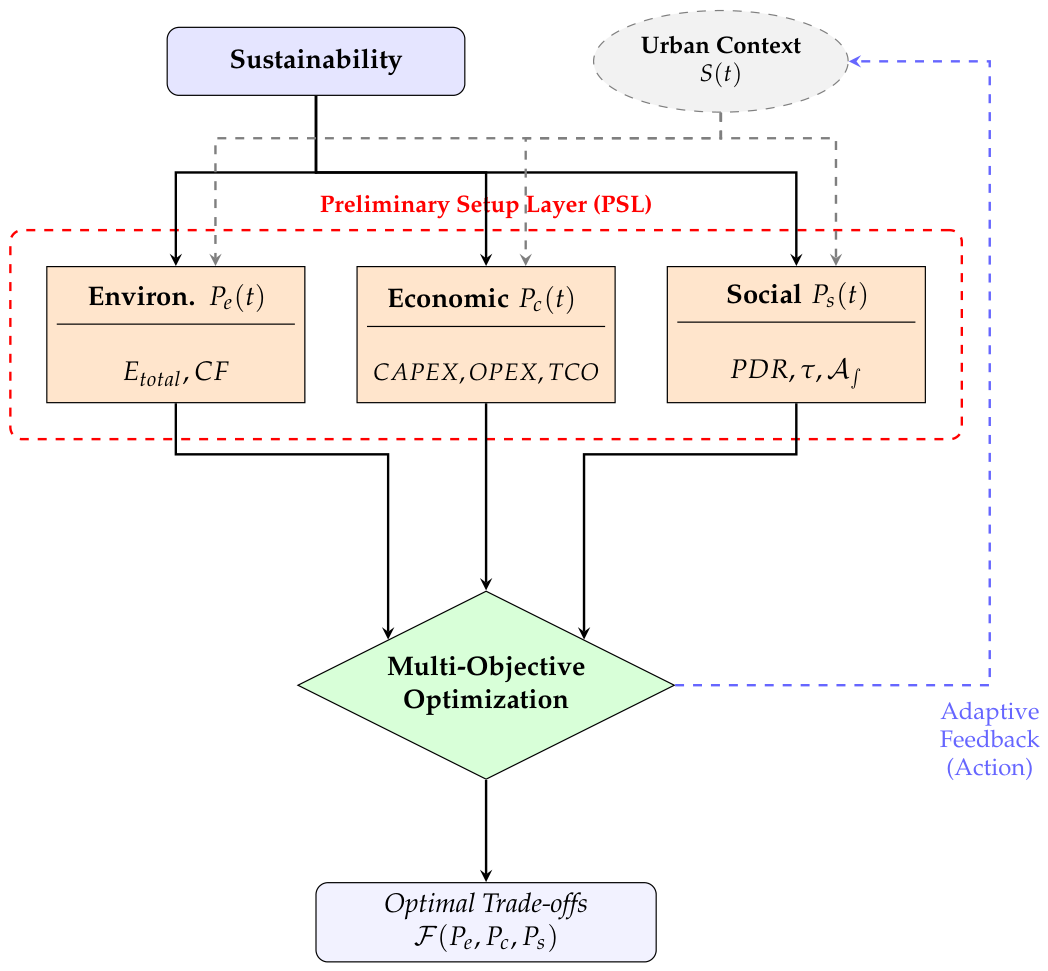
The architecture of the proposed adaptive urban ecosystem is illustrated in Figure 3. The framework conceptualizes the transition from a static sustainability model to a dynamic, context-aware system. As shown in this diagram, the system is driven by two primary inputs: the Sustainability, which defines the theoretical SDG 11, and the Urban Context, providing real-time environmental and operational data. These inputs converge on the Preliminary Setup Layer (PSL), highlighted by the dashed red boundary. Within this layer, the sustainability pillars $P_e\left(t\right)$, $P_c\left(t\right)$, and $P_s\left(t\right)$ are not treated as static metrics but as dynamic functions of the urban context.

The interaction among these pillars is governed by a Multi-Objective Optimization engine. This component processes the input parameters (i.e., from the PSL) to resolve inherent trade-offs, also ensuring that the infrastructure remains efficient and reliable under varying urban conditions. Finally, an Adaptive Feedback loop returns the optimized state to the urban context, enabling a continuous self-healing and self-configuring cycle.

2.2.1. Smart Urban Context

The core of the proposed framework lies in the formalization of the smart urban context as a dynamic CPS ecosystem governed by a state-space representation. Thus, a dynamic urban context $C\left(t\right)$ can be defined as the n-tuple of Equation (1):

$$C\left(t\right)=\left(c_1\left(t\right),c_2\left(t\right),\dots ,c_n\left(t\right)\right)\in \mathcal{C}\subseteq {\mathbb{R}}^n$$

(1)

where each component $c_i\left(t\right)$ represents a specific environmental or systemic metric, such as traffic congestion levels, network availability, or sudden urban emergencies, and where $\mathcal{C}$ is the context state space.

To tune the model to urban-wide areas, usually organized into geographical districts (e.g., urban districts, industrial zones, or residential quarters), a context matrix $S\left(t\right)$ is formally defined by Equation (2):

$$S\left(t\right)=\left(\begin{array}{ccc}{C}_{1,1}\left(t\right)& \dots & C_{1,q}\left(t\right)\\ ⋮& \ddots & ⋮\\ C_{p,1}\left(t\right)& \dots & C_{p,q}\left(t\right)\end{array}\right)\in {\mathcal{C}}^{p,q}\subseteq {\mathbb{R}}^{n,p,q}$$

(2)

mapping $p\ast q>0$ districts of the urban area into the corresponding $C_{i,j}\left(t\right)$ context representing the $i,j$-th geographical district at time t. This formulation ensures that the context matrix $S\left(t\right)$ captures the dynamics of the city and its districts, preserving geographic and topological distance through the matrix adjacency. This allows the municipality to identify spatial correlations and proximity-based dependencies, which are essential for risk prevention (e.g., hydro-geological monitoring) and urban optimization (e.g., commercial promotion in high-footfall areas). Therefore, it is possible to identify complex spatial–temporal correlations that would be lost in a lower-dimensional or aggregated representation, finally identifying optimal trade-offs among the three pillars of sustainability. This representation enables a comprehensive overview of the city dynamics by aggregating localized district-level data and identifying potential spatial correlations between adjacent districts. Using this structured information, the framework can detect criticalities and vulnerabilities associated with specific districts based on the interplay of their context metrics, such as traffic congestion, weather patterns, and crowd density.

The practical implications of such granular monitoring are manifold: high-resolution telemetry is crucial for hydro-geological risk prevention and for optimizing urban traffic planning through proactive interventions; the ability to analyze real-time visitor and tourist flows enables more effective promotion of events and commercial activities in areas with higher crowding; and the high-dimensional observation space is transformed into an actionable decision-support tool, allowing the municipality to identify both systemic risks and strategic opportunities by capturing the inter-dependencies between neighboring districts. This representation does not merely describe the environment but actively shapes the weighting of the sustainability pillars within the proposed multi-objective optimization process, ensuring that the resulting urban trade-offs are both resilient and context-aware. The brain of the optimization process determines the criticality of the current situation. For example, in high-criticality scenarios, the controller may prioritize immediate social and network performance by extending the duration of high-power operational states. Conversely, in routine contexts, the optimization logic shifts toward energy saving and cost reduction. As a result of this analysis, the context impacts the sustainability of the smart urban ecosystem and the selected main metrics that characterize its pillars, as described below. This holistic representation emphasizes that the transition toward a smart city is not merely technological but is intrinsically linked to measurable sustainability goals, where CPSs bridge the gap between physical infrastructure and socio-economic outcomes.

2.2.2. Sustainability Pillars and Metrics

Environmental sustainability $P_e$ is traditionally quantified by the ecological cost of the digital infrastructure, focusing primarily on metrics such as energy consumption and carbon footprint. However, in the context of a smart city, this perspective is inherently limited. True environmental sustainability must be redefined through the proactive role of CPSs, acting as responsive sentinels. Beyond mere device-level energy savings, these systems monitor both local and neighboring contexts to dynamically manage urban dynamics. By anticipating traffic peaks, high-density events, and congestion, the DQN policy prioritizes the systemic prevention of pollution surges, using the infrastructure as an active tool for ecological mitigation rather than a passive energy consumer. In such a scenario, energy consumption is not a static value but a baseline strictly coupled with the operational context $S\left(t\right)$. It serves as a direct measure of the CPS’s impact on environmental and economic costs, as the power consumption scales dynamically across different modes, from low-power stand-by or idle states to high-performance active monitoring.

Let $d_{i,j}$ be the number of devices deployed across the $i,j$-th urban district. The total energy consumption E over an observation interval $[t_0,t]$ is formally defined by Equation (3):

$$E(s,t)={\int }_{t_0}^{t}P(S\left(\tau \right),\tau ),d\tau \left[\mathrm{kWh}\right].$$

(3)

where the lowercase s represents the specific realization of the state at the current time t, i.e., $s=S\left(t\right)$. The total power P is the result of the sum of the instantaneous power measured at time t for each device in the district, formally defined by Equation (4):

$$P(s,t)={\displaystyle \sum _{i=1}^p}{\displaystyle \sum _{j=1}^q}{\displaystyle \sum _{k=1}^{d_{i,j}}}{P}_{i,j,k}(C_{i,j}\left(t\right),t)\left[\mathrm{W}\right].$$

(4)

The carbon footprint ($CF$) represents the Global Warming Potential (GWP) [56] associated with the system’s existence and operation in the observation interval $[t_0,t]$. It accounts for the embodied carbon of each device, provided as a manufacturer specification, and the emissions derived from its contextual energy consumption. Leveraging the energy formulation defined in Equation (3), the total $CF$ for the infrastructure across the n districts is formalized by Equation (5):

$$CF(s,t)={\displaystyle \sum _{i=1}^p}{\displaystyle \sum _{j=1}^q}{\displaystyle \sum _{k=1}^{d_{i,j}}}GW{P}_{i,j,k}+{ϵ}_{geo}·E(s,t)\left[{\mathrm{kgCO}}_2\mathrm{eq}\right]$$

(5)

where $GW{P}_{i,j,k}$ is the aggregate cradle-to-gate carbon footprint of the k-th device located in the $i,j$-th urban district (including its enclosure, electronics, and battery, where applicable). This term represents the embodied impact linked to the physical existence of the device. The term ${ϵ}_{geo}·E(s,t)$ represents the operational impact, where ${ϵ}_{geo}$ denotes the grid emission intensity factor [57], and $E(s,t)$ is the context-dependent energy consumption derived from the instantaneous power $P(s,t)$, as defined by Equation (3). This formulation allows the framework to evaluate how the selection of specific hardware models and their operational duty cycles, driven by the urban dynamics captured in $S\left(t\right)$, jointly influence the total environmental sustainability of the infrastructure.

The economic sustainability ($P_c$) ensures the financial viability and scalability of the infrastructure within municipal budget constraints. It is modeled through the Total Cost of Ownership (TCO), which balances the initial investment with long-term maintenance. The TCO represents the comprehensive financial metric for evaluating the $P_c$ of the CPS infrastructure over its entire operational life. It is defined by Equation (6) as the sum of the initial investment and the accumulated operating costs:

$$TCO(s,t)=CAPEX\left(t_0\right)+OPEX(s,t))\left[\mathrm{Currency}\right]$$

(6)

The term $CAPEX\left(t_0\right)$ represents the capital expenditure incurred at the initial time $t_0$, acting as a static and context-independent value. It includes the procurement of devices for all the districts, including hardware costs, licenses, and physical installation. By defining it at $t_0$, the model treats the initial investment as a fixed boundary condition for the optimization problem, as formally defined by Equation (7):

$$CAPEX\left(t_0\right)={\displaystyle \sum _{i=1}^p}{\displaystyle \sum _{j=1}^q}{\displaystyle \sum _{k=1}^{d_{i,j}}}\left(H_{i,j,k}+I_{i,j,k}+L_{i,j,k}\right){|}_{t_0}\left[\mathrm{Currency}\right]$$

(7)

where $H_{i,j,k}$, $I_{i,j,k}$, and $L_{i,j,k}$ denote the hardware, installation, and licensing costs for the k-th device in the $i,j$-th geographical district, respectively.

Conversely, $OPEX(s,t)$ represents the dynamic and context-aware operational expenditure. It is formally defined by Equation (8):

$$OPEX(s,t)={\displaystyle \frac{(t-t_0)}{T}}·K_T+OPE{X}_V(s,t)\left[\mathrm{Currency}\right]$$

(8)

where the $K_T$ term represents the time-invariant operational costs (e.g., cloud subscription fees or fixed infrastructure leasing) in period T. The variable operational expenditure $OPE{X}_V$ during the observation interval $[t_0,t]$ is formally defined by Equation (9) as a direct function of the geographical urban context, capturing how urban dynamics drive resource allocation and energy demand.

$$OPE{X}_V(s,t)={\int }_{t_0}^t\left({\displaystyle \sum _{i=1}^p}{\displaystyle \sum _{j=1}^q}{\displaystyle \sum _{k=1}^{d_{i,j}}}\left[V_{i,j,k}\left(\tau \right)·P_{i,j,k}(C_{i,j}\left(\tau \right),\tau )+\left(M_{i,j,k}\left(\tau \right)+{\delta }_k·B_{i,j,k}\left(\tau \right)\right)·{\mathcal{O}}_{pred}(C_{i,j}\left(\tau \right),\tau )\right]\right)d\tau$$

(9)

In this formulation, the first term of the sum captures the monetary cost of the energy, where $V_{i,j,k}$ is the unit price (currency per kW), and $P_{i,j,k}$ is power from Equation (4). The integral term also captures the localized maintenance and hardware preservation costs across the districts over the observation interval $[t_0,t]$. Here, $M_{i,j,k}$ denotes the routine maintenance for the k-th device in the $i,j$-th district, encompassing inspections and standard operational overhead. The second part of the sum addresses the critical management of power-source longevity. The binary parameter ${\delta }_k$ indicates the presence of a battery for the k-th device model, as specified by Equation (10).

$${\delta }_k=\left\{\begin{array}{cc}1\hfill & \mathrm{if}\mathrm{the}k\text{-}\mathrm{th}\mathrm{device}\mathrm{is}\mathrm{battery}\text{-}\mathrm{powered}\hfill \\ 0\hfill & \mathrm{if}\mathrm{the}k\text{-}\mathrm{th}\mathrm{device}\mathrm{is}\mathrm{mains}\text{-}\mathrm{powered}.\hfill \end{array}\right.$$

(10)

The term $B_{i,j,k}\left(t\right)$ represents the replacement cost for the battery (including procurement and field logistics). These factors are modulated by the predictive operator ${\mathcal{O}}_{pred}$, which estimates the degradation rate and the “state of health” of the device. By incorporating this predictive logic, the model acknowledges that operational stress directly accelerates battery chemical aging. The above formulation is useful for long-term planning, as battery-operated devices (${\delta }_k=1$) can incur periodic replacement costs and labor, whereas mains-powered devices (${\delta }_k=0$) contribute more significantly to the energy cost.

Social sustainability ($P_s$) is evaluated through the system’s ability to provide a reliable and timely service to the community. Information systems and IT services are increasingly performing a wide variety of organizational functions and personal activities. Therefore, high-quality information systems and IT services are essential to provide value and avoid possible negative consequences for their stakeholders. According to the System Quality and Software Quality Requirements and Evaluation (SQuaRE) family of the International Organization for Standardization (ISO)/International Electrotechnical Commission (IEC) [58], the social value of a CPS is quantified through objective Quality of Service (QoS) parameters. In this work, we redefine these metrics to be context-aware, ensuring they respond dynamically to the urban context. A QoS metric is the Packet Delivery Ratio (PDR) measuring the communication integrity and reliability of the data flow from the devices to the application. It is formally defined by Equation (11):

$$PDR(s,t)={\displaystyle \frac{{\int }_{t_0}^t{\sum }_{i=1}^p{\sum }_{j=1}^q{\sum }_{k=1}^{d_{i,j}}{\mathsf{\Psi }}_{RX,I,j,k}(S\left(\tau \right),\tau )d\tau }{{\int }_{t_0}^t{\sum }_{i=1}^p{\sum }_{j=1}^q{\sum }_{k=1}^{d_{i,j}}{\mathsf{\Psi }}_{TX,I,j,k}(S\left(\tau \right),\tau )d\tau }},t-t_0\gg {\tau }_{max}$$

(11)

where the $PDR$ is defined as the ratio of cumulative successfully received packets (${\mathsf{\Psi }}_{RX}$) to total transmitted packets (${\mathsf{\Psi }}_{TX}$) across the urban scenario. By modeling these variables as time-varying processes, the integral structure captures the cumulative throughput over the observation window $[t_0,t]$, effectively filtering out instantaneous stochastic noise. To ensure statistical consistency, the interval $[t_0,t]$ is assumed to be significantly larger than the maximum network propagation delay. Furthermore, the explicit dependence of both integrals on the urban context $S\left(t\right)$ formalizes how urban stressors, such as localized fading or congestion, modulate this ratio.

${\tau }_{max}$ is defined by Equation (12):

$${\tau }_{max}=\underset{i,j,k}{\max }{\tau }_{Prop,i,j,k}\left(t\right)$$

(12)

where the term ${\tau }_{Prop,i,j,k}\left(t\right)$ denotes the instantaneous latency experienced by a packet transmitted by the k-th device within the $i,j$-th district. This delay accounts for the physical distance between nodes, the signal propagation speed in the urban medium, and potential context-driven retransmissions or multi-hop overheads.

Service Timeliness, denoted as $\sigma (s,t)$, quantifies the average end-to-end latency over the observation window $[t_0,t]$, ensuring that the system meets specific real-time requirements. It is formally defined by Equation (13) as the mean temporal gap between data generation at the sensing layer and its final reception at the application level:

$$\sigma (s,t)=\mathbb{E}{\left[t_{D,i,j,k}-t_{S,i,j,k}\right]}_{(t-t_0)}\left[\mathrm{s}\right]$$

(13)

where $t_S$ and $t_D$ represent the timestamps of data sensing and delivery for each packet, respectively. To maintain the operational integrity of safety-critical services, we impose a strict latency constraint:

$$\sigma (s,t)\le {\tau }_{req}$$

(14)

where ${\tau }_{req}$ represents the application-specific deadline. While ${\tau }_{max}$ in Equation (12) defines the physical upper bound of the network propagation delay, the timeliness $\tau$ accounts for the total system latency, including processing times and queuing delays. The condition $\sigma \le {\tau }_{req}$ ensures that the response of the system to the urban environment $S\left(t\right)$ is based on timely rather than outdated information to preserve the effectiveness of the decision-making process under dynamic conditions.

Service Availability (${\mathcal{A}}_s$) [58] represents the fraction of time the infrastructure is fully operational and capable of fulfilling its functional requirements. Although service availability at an individual device level is sensitive to localized stressors, ${\mathcal{A}}_s$ is a critical system-level Key Performance Indicator (KPI). The proposed model leverages the aggregation of individual availability metrics to derive a systemic indicator that reflects the capacity of the smart city infrastructure to provide continuous services, despite possible failures of single nodes.

The availability of a device $a_k$ is defined by Equation (15):

$$a_k\left(t\right)={\displaystyle \frac{Uptim{e}_k(t,t_0)}{Downtim{e}_k(t,t_0)+Uptim{e}_k(t,t_0)}}$$

(15)

where $Uptim{e}_k(t,t0)$ denotes the cumulative duration within the time interval $(t_0,t)$ in which the k-th device is fully operational and the service is active. Conversely, $Downtim{e}_k(t_0,t)$ accounts for periods of inactivity, and the service is inactive. Thus, the system-level availability is formally specified by Equation (16):

$${\mathcal{A}}_s(s,t)={\displaystyle \sum _{i=1}^p}{\displaystyle \sum _{j=1}^q}{\displaystyle \frac{1}{d_{i,j}}}{\displaystyle \sum _{k=1}^{d_{i,j}}}{a}_{i,j,k}\left(t\right)$$

(16)

where $d_{i,j}$ denotes the number of devices deployed across the $i,j$-th urban district. Unlike static reliability models, this formulation accounts for environmental and operational stressors across the full urban context $S\left(t\right)$. A high ${\mathcal{A}}_s$ value is mandatory for mission-critical urban services, ensuring 24/7 availability and resilience to localized disruptions.

2.2.3. DQN-Based Optimization

A DQN-based optimization strategy has been adopted to achieve context-aware governance of urban resources, thereby facilitating the transition toward more adaptive and sustainable cities. To reconcile the high computational demands of DL with the strict resource and energy constraints of localized municipal infrastructures, the proposed framework decouples the operational pipeline into two distinct phases: offline training and online edge inference (i.e., on edge gateway devices).

During training, the neural network iteratively processes environmental and behavioral data over a total-episode horizon, minimizing the loss until stable policy convergence is achieved. Once the learning process is complete, the optimized policy configuration is extracted and deployed directly onto the edge gateways for the inference phase. During this live deployment, the edge nodes execute lightweight, deterministic forward-pass mappings to select the optimal structural configuration in real time, thus minimizing local power consumption.

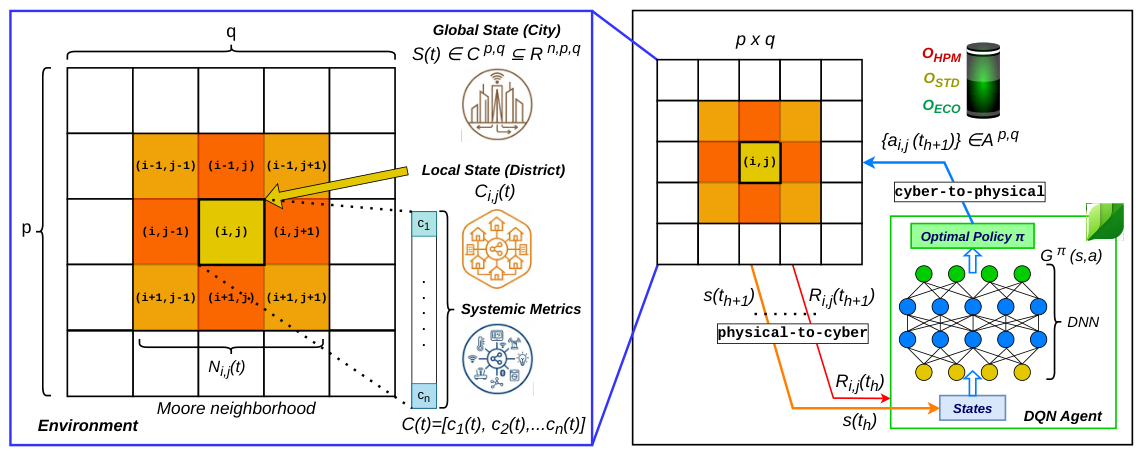
A general schema of the proposed method is depicted in Figure 4. This architectural framework transitions from raw environmental data to a high-level decision-making state through a three-level hierarchical abstraction. At the most granular level (System Metrics), the system captures systemic metrics represented as $c_n\left(t\right)$. Such metrics are geographically aggregated into $p·q>0$ district contexts ($C_{i,j}\left(t\right)=(c_1\left(t\right),c_2\left(t\right),\dots ,c_n\left(t\right))$) encapsulating the n multi-dimensional status of the $i,j$-th district at time t.

The integration of this state representation into the DQN pipeline follows a specific information flow. The Environment block, acting as the CPS, outputs the context matrix $S\left(t\right)$. Therefore, the matrix $S\left(t\right)$ is passed to the DQN agent, which processes the data based on its internal structure. It uses convolutional layers to keep the grid shape intact. This allows the agent to recognize spatial patterns, such as how a problem in one district might affect its neighbors. By preserving this grid structure, the agent better understands the layout of the city, leading to more effective urban management decisions.

More specifically, at each time step t, the agent observes the global state of the city through the context matrix $S\left(t\right)\in {\mathcal{C}}^{p,q}$. This representation captures the status of all functional districts $(i,j)$, characterized by systemic metrics whose raw data, collected from IoT devices, are normalized before being processed by the DNN to ensure numerical stability and effective feature extraction. Once the agent detects the optimal policy for the devices of each district $(i,j)$, it transforms this policy into an operational action $a_{i,j}\in A^{p,q}$ to set devices to a specific operational condition. By discretizing the operational conditions into a finite set of $h\in \mathbb{N}$ operational modes, as defined by Equation (17),

$$O=\{{\mathbf{o}}_1,\dots ,{\mathbf{o}}_h\},{\mathbf{o}}_h\in \mathbb{N}$$

(17)

the action $a_{i,j}$ can be defined as a pair in Equation (18):

$$a_{i,j}=(o_s,o_f)\in A^{p,q}\subseteq O^2$$

(18)

with $o_s,o_f\in O$ as the starting and final states of the action. It is important to remark that, in general, the operational conditions are usually orthogonal to the sustainability pillars, and $o_s$ may be the same as $o_f$; i.e., no changes are enforced by $o_s=o_f$ actions.

The sustainability gain $G^{\pi }(s,a)$ is formally defined by Equation (19) for a specific state–action pair $(s,a)\in SxA$. It is the expected cumulative discounted return, which the DQN agent aims to maximize to identify the optimal policy ($\pi$). Specifically, $G^{\pi }(s,a)$ corresponds to the action-value function satisfying the Bellman optimality criterion [59].

$$G^{\pi }(s,a)=\mathbb{E}\left[{\displaystyle \sum _{y=0}^{\infty }}{\gamma }^y{\displaystyle \sum _{i=1}^p}{\displaystyle \sum _{j=1}^q}{\mathcal{R}}_{i,j}\left(S(t+y),A(t+y)\right)\right],\gamma \in (0,1)$$

(19)

This formulation encapsulates the multi-level complexity of urban infrastructure through several key components. The expectation operator $\mathbb{E}[·]$ accounts for the intrinsic stochasticity of the urban environment. State transitions and the resulting rewards are influenced by unpredictable events, such as traffic spikes or sudden emergencies, which characterize the described dynamics. The temporal index t denotes the current decision epoch, while $y\in \mathbb{N}$ represents the discrete look-ahead horizon. The term $t+y$ indicates that the agent’s current return is not merely a function of immediate rewards but a discounted accumulation of expected future states $S(t+y)$ and actions $A(t+y)$. The integration of an infinite horizon ($y\to \infty$), moderated by the discount factor $\gamma \in (0,1)$, ensures the strategic sustainability of the policy: for $\gamma \to 0^{+}$, the objective function collapses into a single-step optimization, where the agent considers only the immediate reward. Conversely, as $\gamma \to 1^{-}$, the agent equally weights present and future rewards. However, in this case, the agent loses the ability to rank different strategies, as any policy providing a positive reward would result in the same mathematical value (∞). By keeping $\gamma <1$, the series converges to a finite number, allowing the DQN to mathematically determine which policy is superior by comparing finite values.

The sustainability gain $G^{\pi }(s,a)$ aggregates the local rewards ${\mathcal{R}}_{i,j}$ at the $i,j$-th district level to ensure computational scalability within large-scale smart city deployments. As the number of urban IoT devices may grow into the thousands, a device-level reward structure would introduce high-frequency noise and a dimensional explosion in the feedback signal, severely impacting the DQN convergence. Through a district-level reward ${\mathcal{R}}_{i,j}$, the system considers each geographical area as a functional domain. This ensures that the learning complexity remains tied to the resolution of the urban ($p\times q$) grid rather than the fluctuating density of the deployed hardware. It is formally defined by Equation (20), aggregating the environmental, economic, and social sustainability metrics of all devices within that area:

$$\begin{array}{c}{\mathcal{R}}_{i,j}(s,a)=1.0-\left[{\lambda }_1{\mathcal{L}}_{\mathrm{e}}({\eta }_{i,j},a_{i,j})+{\lambda }_2{\mathcal{L}}_{\mathrm{c}}({\eta }_{i,j},a_{i,j})+{\lambda }_3{\mathcal{L}}_{\mathrm{s}}({\eta }_{i,j},a_{i,j})\right]\end{array}$$

(20)

where ${\lambda }_k\in [0,1]\subset \mathbb{R}$ are the sustainability factors balancing the impact of normalized losses $\mathcal{L}$ on the system, such that ${\sum }_{k=1}^3{\lambda }_k=1$. Each factor ${\lambda }_k$ sets a specific firmware operating level, adjusting the device sampling interval and the transmission duty cycle. Specifically, ${\lambda }_1$ maximizes deep-sleep periods; ${\lambda }_2$ restricts transmission windows to limit hardware stress and meet regulatory caps; and ${\lambda }_3$ enables high-frequency sampling to capture fine-grained urban dynamics. The reward function ${\mathcal{R}}_{i,j}$ formalizes the operational efficiency of the $(i,j)$-th district by coupling the local action $a_{i,j}$ with the expanded neighborhood [60] state $\left({\eta }_{i,j}\right)$. This formulation adopts a penalty-from-unity approach: starting from an ideal value of 1.0, the reward is decreased by a weighted sum of these components. As a consequence, maximization of the expected return $G^{\pi }(s,a)$ is mathematically equivalent to minimizing the long-term cumulative loss. Here, a policy $\pi$ is a parametric configuration identified by the 3-tuple in Equation (21):

$$\pi =({\lambda }_1,{\lambda }_2,{\lambda }_3)$$

(21)

The spatial dependency is modeled upon the Moore neighborhood convention, which is widely adopted in networked RL to capture local inter-dependencies and interference patterns in distributed sensing infrastructures [60]. It is formally defined by Equation (22):

$$\eta (i,j)=\{C_{u,v}\in \mathcal{S}:|u-i|\le r,|v-j|\le r\}$$

(22)

where $\eta (i,j)$ is composed of the context subset (sub-matrix) of the global state space $\mathcal{S}$ centered on the district $(i,j)$ with radius r. The Moore neighborhood can include nodes along the diagonal directions, bounding the maximum Euclidean distance to the central node within $\sqrt{2}$ spatial units. This geometric extension provides a significantly closer topological approximation to a continuous circular area compared to the 4-cell Von Neumann alternative, which is strictly constrained by the Manhattan distance. Moreover, the Moore neighborhood allows the framework to capture diagonal movements and multi-directional flows across the urban grid.

By conditioning environmental (${\mathcal{L}}_{\mathrm{e}}$), economic (${\mathcal{L}}_{\mathrm{c}}$), and social (${\mathcal{L}}_{\mathrm{s}}$) losses on the context of adjacent districts, the system prevents the emergence of selfish policies that might optimize local parameters at the expense of neighboring areas. Each loss component ${\mathcal{L}}_x$ of Equation (20) is modeled as a weighted aggregation of a specific subset of normalized metrics, as specified by Equation (23):

$${\mathcal{L}}_x={\displaystyle \sum _{k=1}^n}{\omega }_k·{\widehat{c}}_k;{\widehat{c}}_k={\displaystyle \frac{c_k}{c_k^{max}}}$$

(23)

where ${\omega }_k$ represents the relative weight of each normalized metric ${\widehat{c}}_k$ within that specific loss, such that ${\sum }_{k=1}^n{\omega }_k=1$, and $c_k^{max}$ is the maximum value threshold allowed to preserve the operation of the equipment. The hierarchical weighting structure allows the DQN agent to internalize a complex multi-dimensional state while maintaining a clear balance between high-level sustainability goals and specific physical constraints.

3. Case Study

To validate the feasibility of the proposed framework, a real-world urban deployment consisting of five neighboring districts within the historical center of Caltanissetta (Sicily, Italy) is investigated.

3.1. Experimental Setup

An extensive, long-term physical deployment that utilizes heterogeneous sensors and gateways allows for a rigorous field validation that synthetic simulations cannot replicate, capturing unpredictable environmental anomalies and real-world hardware degradation. To demonstrate the effectiveness of our framework, we adopt LoRaWAN [18] as the reference smart city ICT infrastructure. This LPWAN standard is specifically engineered to connect low-power, battery-operated devices to regional or national networks, supporting key operational requirements like bi-directional communication and end-to-end security [61]. The selection of this testbed was driven by its structural and morphological complexity rather than simple physical availability. Historic European city centers present severe signal propagation challenges for LPWANs due to heavy stone masonry, narrow street canyons, and irregular elevation profiles. Demonstrating that our DQN agent can discover optimal operational trade-offs and overcome these radio propagation hurdles establishes a robust, “worst-case” benchmark.

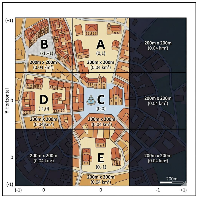
As shown in Figure 5, a $3\times 3$ map defines the urban domain, where districts A, B, C, D, and E represent the active operational area covered by a central LoRaWAN gateway located in district C(0,0).

Each cell corresponds to a surface area of 0.04 km², due to the urban morphology of the historic center and its impact on the LoRaWAN communication. To ensure the replicability of the proposed approach, the cell size can be appropriately scaled based on the topology and geo-morphological features of the new monitored environment. Non-covered peripheral areas are masked to focus the DQN agent policy on the core interconnected districts. To model the spatial relationships between distributed edge gateways without loss of generality, the urban environment is structured via a uniform two-dimensional spatial tessellation. Within this discrete grid, each cell defines the nominal coverage domain of a specific gateway deployment.

The spatial interaction and localized state-sharing among adjacent nodes are governed by a Moore neighborhood of radius $r=1$. Formally, for a gateway located at cell coordinates $(x_0,y_0)$, the set of observable neighboring cells ${\mathcal{N}}_{(x_0,y_0)}$ is defined by Equation (24):

$${\mathcal{N}}_{(x_0,y_0)}=\{(x,y)\in {\mathbb{Z}}^2:|x-x_0|\le 1,|y-y_0|\le 1\}\setminus \left\{(x_0,y_0)\right\}$$

(24)

Although the grid structure is uniform to keep the algorithm scalable, all real-world asymmetries (e.g., traffic changes or signal obstructions) are dynamically captured inside the DRL state vector. As a result, the DQN agent learns to break the geometric symmetry at runtime, weighting each neighbor based on its real-time link quality and traffic density. The agent can anticipate incoming data traffic from neighboring areas and adjust settings in advance to stay within the constraints.

Each active district is equipped with one installation point (pole) including several IoT devices to capture the multi-faceted dynamics of the district, as reported in

Table 5. Spatial distribution and functional roles of the urban sensing infrastructure across the five neighboring districts and the centroidal gateway (GW).

District/Pole	Coord. $(\mathit{i},\mathit{j})$	Deployed Devices	Strategic Role
A	$(0,1)$	1 Env., 1 Traffic, 1 Parking	Integrated Urban Sensing
B	$(-1,1)$	1 Env., 1 Traffic	Telemetry & Flow Analysis
C	$(0,0)$	1 Env., 1 Traffic, 1 Parking, 1 GW	Network Backbone & Sensing
D	$(-1,0)$	1 Traffic, 2 Parking	Mobility & Occupancy Hub
E	$(0,-1)$	1 Parking	Localized Spot Monitoring

.

More specifically, Pole A acts as an integrated sensing cluster hosting one environmental station, one traffic sensor, and one parking node, while Pole B provides a dual-source setup for environmental and traffic monitoring. A similar configuration is replicated on Pole C, which hosts an additional environmental station, a traffic sensor, a parking node, and a standalone LoRaWAN gateway providing the backbone for the LoRaWAN communication layer. Mobility dynamics are further captured by Pole D, which serves as a high-density hub with one traffic sensor and two parking nodes, and by Pole E, conceived for localized parking monitoring with a single sensing unit.

Thus, the experimental testbed comprises 12 heterogeneous edge devices and a central gateway $GW$, leveraging hardware and firmware technology provided by the innovative company SmartMe.io (https://smartme.io/) (accessed on 24 June 2026). The gateway acts as the primary orchestrator, ensuring seamless connectivity between the edge nodes and a dedicated cloud-based smart mobility platform for real-time data processing and analytics. This technological infrastructure is categorized into three functional typologies of devices, as shown in

Table 6. Technical specifications and functional classification of the urban IoT testbed.

Typology	Hardware Platform	Num	Primary Function
Environmental (weather station)	Raspberry Pi 4 (12 V supply)	3	Ambient telemetry
Parking (optical sensor)	Nvidia Jetson Nano (5 V rail 1)	5	Optical occupancy sensing
Traffic (optical sensor)	Nvidia Jetson Nano (5 V rail 1)	4	Vehicle flow analysis
Network & Context Parameters
Protocol	LoRaWAN Class C, Spreading Factor 7, 125 kHz, Coding Rate 4/5 2
Duty Cycle	$1\%$ (European EU 868 MHz regional frequency band)

¹ Powered via DC–DC converter from a 24 V source; ² ChirpStack, an open-source LoRaWAN server.

.

All poles are permanently mains-powered, and devices operate in a continuous DC active state. As a consequence, the $OPE{X}_V$ formulation (Equation (9)) is simplified (${\delta }_k=0$).

Table 7. Baseline power and daily (24 h) energy consumption in standard operating mode, without DQN optimization.

Typology	Num	${\mathit{P}}_{\mathit{device}}$ (W)	${\mathit{E}}_{\mathit{device}}$ (kWh)	Num · ${\mathit{E}}_{\mathit{device}}$ (kWh)
Environmental (weather station)	3	2.364	0.0567	0.1702
Parking (optical sensor)	5	3.395	0.0815	0.4074
Traffic (optical sensor)	4	4.460	0.1070	0.4281
LoRaWAN gateway	1	3.583	0.0860	0.0860
Overall benchmark	13	-	0.3312 1	1.0917

¹ It represents the benchmark for the district C (0,0) in our case study.

reports the baseline energy metrics under standard operating conditions, assuming a static duty cycle without any dynamic policy intervention. These values represent the reference consumption against which the agent’s energy-saving capabilities are subsequently measured.

This baseline was established during the start-up phase of the project, when measurements were calibrated and validated using certified instrumentation. Therefore, this baseline is designed to be periodically updated and refined, provided that such updates remain compatible with existing network constraints and infrastructure overhead (e.g., the 1% duty cycle in LoRaWAN communication).

During runtime, the system collects a set of heterogeneous physical measurements from the urban environment, formally defined as a real-valued 10-dimensional tuple by Equation (25):

$$C\left(t\right)=\left(c_1\left(t\right),c_2\left(t\right),\dots ,c_{10}\left(t\right)]\right)\in \mathcal{C}\subseteq {\mathbb{R}}^{10}$$

(25)

in compliance with Equation (1).

Table 8. Set of metrics considered for the examined scenario, with related measures and impacts on the dynamics of the city.

Dataset	Metric	Measure	Impact
Weather	$c_1$	Ambient Temperature (∘C)	Hardware thermal stress and operational efficiency
	$c_2$	Relative Humidity (%)	Signal attenuation and link propagation quality
	$c_3$	Ultraviolet (UV) Index	Seasonal fluctuations and weather-induced variability
Traffic	$c_4$	Flow Index	Real-time service urgency and prioritization
	$c_5$	Total Vehicle Count	Demand intensity and infrastructure load
Parking	$c_6$	Lot Occupancy Rate	Local urban activity density and utility demand
LoRaWAN	$c_7$	Packet Delivery Ratio (PDR)	Network reliability and communication quality
	$c_8$	Latency ($\tau$)	Transmission delay and real-time responsiveness
	$c_9$	RSSI (dBm)	Signal strength and transmission power efficiency
	$c_{10}$	SNR (dB)	Link robustness and noise interference levels

reports the metrics considered for the examined scenario, including features and related impacts on the city dynamics.

The radio parameters ($c_9,c_{10}$) and urban demand indicators ($c_4,c_5,c_6$) specify the transmission power and frequency. In particular, the Received Signal Strength Indicator (RSSI) represents the total received power, including the signal, noise, and interference; the Signal-to-Noise Ratio (SNR) quantifies the ratio between the power of the received signal and the background noise floor.

Physical stressors ($c_1,c_2$) derived from the weather dataset, alongside the Ultraviolet (UV) index ($c_3$), influence the probability of hardware fatigue and maintenance frequency. In our $TCO$ model, these environmental factors directly impact the amortization $OPEX$ and $CAPEX$ by modulating the expected life-cycle of the mains-powered devices. Furthermore, the performance metrics of the LoRaWAN ($c_7,c_8$), combined with the activity density ($c_6$), define the overall $QoS$.

The metrics in Table 8, selected from weather, traffic, parking and LoRaWAN datasets, serve as the primary inputs for the optimization process. To prevent bias during the DQN training phase, these raw observations are normalized into a normalized demand vector $\widehat{C}$, as defined by Equation (23). Through the normalization process, the DQN agent executes the operational phases of its architecture to maximize the cumulative reward $\mathcal{R}$, defined by Equation (20). The training process integrates experience replay and target network synchronization to ensure the stability of the Q-value estimation. To effectively navigate the trade-off between investigating new strategies, a trade-off mechanism allows the agent to explore the state–action space before converging toward the optimal policy $\pi$ maximizing the sustainability gain $G^{\pi }(s,a)$.

Three policies characterizing the agent’s behavioral attitude toward urban dynamics emerge as trade-offs from the multi-objective optimization. We define these policies as lazy, balanced, and responsive.

The lazy policy, ${\pi }_l=(0.6,0.3,0.1)$, identifies an energy-saving- and cost-saving-oriented profile. In this configuration, the DQN agent keeps the devices in a low-power state to minimize energy consumption and reduce the associated economic expenditure. It is simultaneously focused on the device lifespan: by operating primarily in less demanding and less stressful conditions, it preserves the hardware’s electronic integrity. Thus, the system ensures long-term operational resilience by avoiding the thermal and computational stress typical of higher-performance modes. Although this policy safeguards hardware longevity and related costs, it introduces a significant operational risk to the urban scenario: by failing to capture micro-scale traffic fluctuations and peak congestion events, the system underestimates the actual urban stress. As a consequence, it can represent a systemic risk to the community, as decision-makers are provided with insufficient data that masks pollution hotspots and traffic bottlenecks. In summary, the lazy policy achieves device-level resilience impacting the city’s observability and, consequently, its sustainability.

The responsive policy, ${\pi }_r=(0.1,0.3,0.6)$, identifies a social-oriented profile. This configuration is highly sensitive to fluctuations in urban traffic demand; while it accepts higher energy and economic costs at the device level, it minimizes information latency. By operating at peak performance, the system avoids underestimating mobility dynamics, which is crucial to preventing flawed or weak decision-making. In this case study, responsiveness translates into substantial environmental and social benefits: by providing high-resolution monitoring of traffic congestion and parking occupancy, the system enables more effective urban flow management and a reduction in traffic congestion. Consequently, the ability to detect and react to micro-scale mobility fluctuations allows for the targeted mitigation of pollution hotspots. In this configuration, local energy E consumption and capital $CAPEX$ expenditure could be a strategic investment to achieve a systemic reduction in the overall environmental footprint.

Three operational policies characterizing the agent’s behavioral attitude toward urban dynamics emerge as trade-offs from the multi-objective optimization: lazy (${\pi }_l$), balanced (${\pi }_b$), and responsive (${\pi }_r$).

The lazy policy, ${\pi }_l=(0.6,0.3,0.1)$, identifies an energy- and cost-saving profile. By heavily penalizing energy expenditure (${\lambda }_1=0.6$), the DQN agent keeps the edge nodes in low-power states (${\mathbf{o}}_{\mathrm{ECO}}$), minimizing thermal stress and long-term hardware degradation. However, this strategy risks underestimating urban traffic peaks, creating blind spots in systemic pollution monitoring.

Conversely, the responsive policy, ${\pi }_r=(0.1,0.3,0.6)$, models a social-oriented profile. By shifting the penalty toward information latency (${\lambda }_3=0.6$), the agent prioritizes real-time observability over energy costs. This configuration triggers maximum sampling and edge-inference rates (${\mathbf{o}}_{\mathrm{HPM}}$), offering high-resolution data crucial for traffic management and localized emission mitigation.

Finally, the balanced policy, ${\pi }_b=(0.3,0.4,0.3)$, defines a nominal baseline profile. It prevents data scarcity without causing severe energy spikes, offering a stable trade-off for routine smart city operations.

The explicit penalty configurations for these operational profiles are formalized in

Table 9. DQN optimization weight configurations for the operational policies.

Policy Profile	${\mathit{\lambda }}_1$	${\mathit{\lambda }}_2$	${\mathit{\lambda }}_3$	Primary Objective
Lazy (${\pi }_l$)	0.6	0.3	0.1	Cost & hardware preservation
Balanced (${\pi }_b$)	0.3	0.4	0.3	Nominal operational baseline
Responsive (${\pi }_r$)	0.1	0.3	0.6	Fine-grained observability

. The weight settings for ${\pi }_l$ and ${\pi }_r$ represent opposite operating boundaries. Specifically, ${\pi }_l$ establishes the upper bound for cost and hardware preservation (${\lambda }_1=0.6$) against the worst-case scenario for fine-grained observability (${\lambda }_3=0.1$). Conversely, ${\pi }_r$ reverses these priorities, evaluating the framework under peak tracking conditions (${\lambda }_3=0.6$) against the worst case for cost and hardware preservation (${\lambda }_1=0.1$). Within this evaluation stress test, ${\lambda }_2$ is constrained between $0.3$ and $0.4$ to satisfy the normalization condition. Maintaining ${\lambda }_2$ as a stable baseline across these extreme configurations guarantees that, even under maximum polarization, the DQN agent is intrinsically bound to respect regulatory telecommunication constraints (e.g., the LoRaWAN’s 1% DC in the EU 868 MHz regional frequency band).

The experimental setup implements three ($h=3$) discrete operational conditions for the edge infrastructure, as defined by Equation (26), specializing Equation (17):

$$O=\{{\mathbf{o}}_{\mathrm{ECO}},{\mathbf{o}}_{\mathrm{STD}},{\mathbf{o}}_{\mathrm{HPM}}\}$$

(26)

where each mode $o_{ECO}$, $o_{STD}$, and $o_{HPM}$ defines a specific power profile. The $o_{ECO}$ mode identifies the lower operational bound for the edge device, characterized by a power consumption of ≈2 W. From a hardware perspective, this configuration corresponds to an idle state or a low-power duty cycle where GPU-intensive tasks are suspended and sensing frequencies are minimized. In the $o_{STD}$ mode, the device operates at its nominal power profile of ≈4 W. This setup ensures compliance with standard regulatory limits while providing sufficient data granularity for routine urban monitoring. The $o_{HPM}$ mode is characterized by maximum computational and transmission effort to ensure high system responsiveness during urban emergencies or peak demand. In this configuration, the device enables full real-time edge inference, resulting in a power surge of ≈7 W. This value aligns with the 10 W thermal design power profile of the Jetson Nano, accounting for sustained GPU utilization during complex neural inference.

3.2. DQN Verification and Validation

The DQN agent training process was executed offline on an Intel(R) Core(TM) i7-7600U × 4 CPUs @ 2.80 GHz and 16 GiB RAM DDR-4, equipped with a Linux Ubuntu 24.10 machine, utilizing empirical historical datasets collected from the Caltanissetta urban testbed. The process was monitored using the operational configurations summarized in

Table 10. DQN training configuration.

Hyperparameter/Metric	Value/Operational Setting
Network Architecture	Fully Connected Multi-Layer Perceptron
Total Training Episodes	1000
Optimization Loss Criteria	MSBE loss, Huber loss
Optimization Algorithm	Adam Optimizer
Exploration Strategy	Exponential $ϵ$-greedy (Epsilon)
Initial Exploration Rate	1.0
Minimum Exploration Rate	0.1
Epsilon Decay Factor	0.995
Target Network Update Pattern	Hard Update (Every Episode)
Discount Factor	0.99
Mini-Batch Size	64
Learning Rate	$1\times {10}^{-4}$

.

To guarantee mathematical precision and numerical convergence within the highly stochastic urban CPS, the agent updates its neural network parameters by tracking the optimization loss trajectory. Minimizing this error ensures that the autonomous controller accurately estimates long-term cumulative rewards, thereby preventing training instabilities and ensuring balanced trade-offs between the environmental, economic, and social sustainability pillars ($P_e,P_c,P_s$).

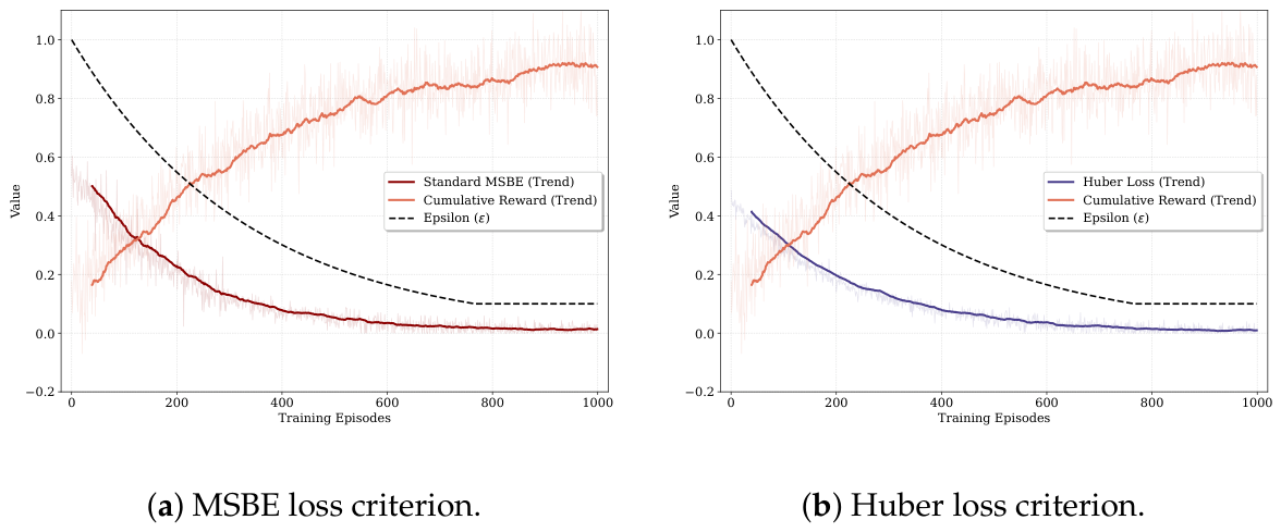
To provide a rigorous validation of this optimization process, a comparative performance analysis was executed between the standard Mean Squared Bellman Error (MSBE) [59] and the Huber loss criterion, as visually contrasted in Figure 6. Although both metrics share the same global minimum, where the Bellman TD error ($\delta$) [62] equals zero, they exhibit significantly different sensitivities to data volatility.

As illustrated in Figure 6, the learning dynamics exhibit three distinct operational phases structurally governed by the exponential decay of the Epsilon curve, which modulates the exploration–exploitation trade-off from $1.0$ down to $0.1$ around episode 700. During the initial stochastic exploration phase (episodes 0–200), where the agent is forced to thoroughly explore the high-dimensional state–action space, the Cumulative Reward remains bounded within a low initial baseline (≈0.15).

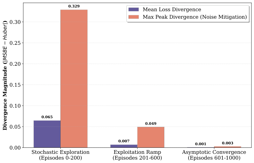
However, within this exploratory window, the mathematical divergence between the two loss criteria becomes evident. The standard MSBE penalizes deviations quadratically (${\delta }^2$), heavily amplifying isolated traffic anomalies or network packet drops. High-frequency noise and sudden sharp spikes up to a raw loss peak of approximately $0.55$ are depicted in Figure 6a. In contrast, the Huber loss (Figure 6b) dampens these shocks by applying a linear penalty to large errors ($\left|\delta \right|>1$), producing a significantly smoother and more stable training curve.

During the central optimization and exploitation ramp phase (episodes 200–600), the progressive decay of Epsilon shifts the agent toward the exploitation of the learned behavior. This transition is characterized by a sharp monotonic increase in the Cumulative Reward, climbing rapidly from ≈0.20 to $0.80$, which is synchronized with a consistent downward trajectory in both loss trends. This simultaneous convergence shows that the neural network successfully approximates the optimal action-value function $G^{\pi }(s,a)$.

Finally, during the plateau phase of asymptotic convergence in the last 200 episodes, the performance metrics reach a definitive steady state. The loss values approach zero, while the Cumulative Reward stabilizes at a high plateau of approximately $0.9$. Crucially, as the Bellman error drops within the unit threshold ($\left|\delta \right|\le 1$), the Huber loss naturally aligns with the MSBE definition. This asymptotic equivalence guarantees numerical stability during the early learning stages without compromising the mathematical precision of the final control policy distributed to the edge devices for local inference.

The empirical phase-by-phase quantification of the divergence between the different learning intervals is quantitatively formalized in Figure 7.

4. Results and Discussion

To account for seasonal variations in traffic–parking patterns and environmental conditions, four representative months have been selected to sample the annual operational cycle from August 2025 to March 2026: August (summer), October (autumn), January (winter), and March (spring). This seasonal sampling ensures that the DQN policy is not over-fitted to specific temporal conditions but remains effective and generalized across different climatic and social contexts. The following analysis details the behavioral patterns learned by the DQN agent across the four representative months, illustrating how the lazy, balanced, and responsive policies map the normalized traffic demand to specific operational conditions $O=\{o_{ECO},o_{STD},o_{HPM}\}$.

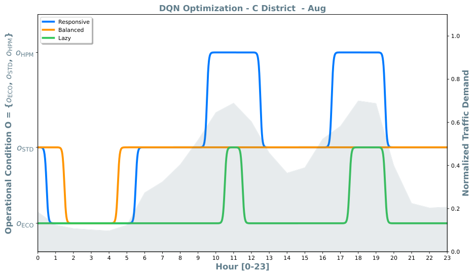
In the August scenario depicted in Figure 8, the agent faces distinct summer traffic peaks, where the policies exhibit highly differentiated behaviors. The lazy policy is in the $o_{ECO}$ state for the majority of the day, showing high tolerance for traffic increases and transitioning to $o_{STD}$ only during the midday and evening peaks. The balanced policy serves as a stable baseline, remaining in $o_{STD}$ for almost the entire 24 h cycle to ensure constant monitoring. Finally, the responsive policy acts as a vigilant sentinel, proactively switching to $o_{HPM}$ during the two main traffic surges.

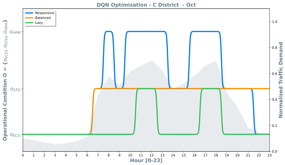
In the October scenario depicted in Figure 9, the lazy policy switches from the $o_{ECO}$ mode to the $o_{STD}$ mode only during the two highest peaks of the day, maintaining its low-power profile as in August. The balanced policy remains in $o_{STD}$ throughout the active city hours (07:00–21:00), reverting to $o_{ECO}$ only late at night. The responsive policy switches to $o_{HPM}$ at each traffic peak, specifically targeting the early morning rush, the midday plateau, and the evening return, thus maximizing the permanence in the high-performance $o_{HPM}$ condition.

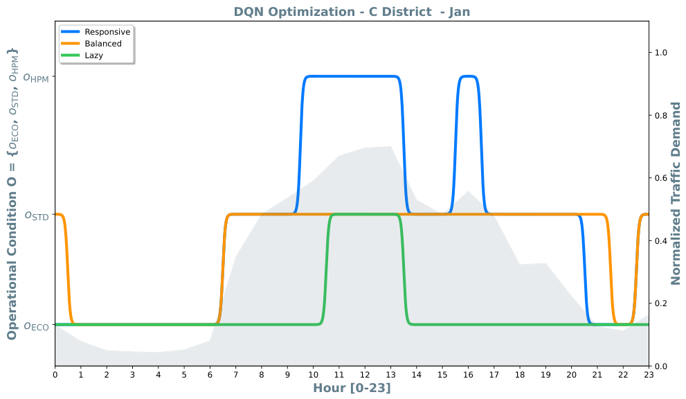
The analysis of the January scenario depicted in Figure 10 reveals how the agent adapts to winter traffic demand. The lazy policy confirms the extreme cost-oriented attitude observed in August and in October. Devices remain in $o_{ECO}$ even during significant traffic demand, with only a brief transition to $o_{STD}$ during the late morning. Although the balanced policy is not highly responsive to the midday peaks (0.5–0.7) in traffic demand, it maintains devices in $o_{STD}$ during the daily period (07:00–21:00) when the city center is expected to be persistently affected by vehicular traffic flows. Devices are switched to $o_{ECO}$ during the early morning hours (normalized traffic demand <0.1) and at around 22:00. The responsive policy, instead, promptly escalates to $o_{HPM}$ to cover the broad midday traffic plateau and a spike at around 16:00.

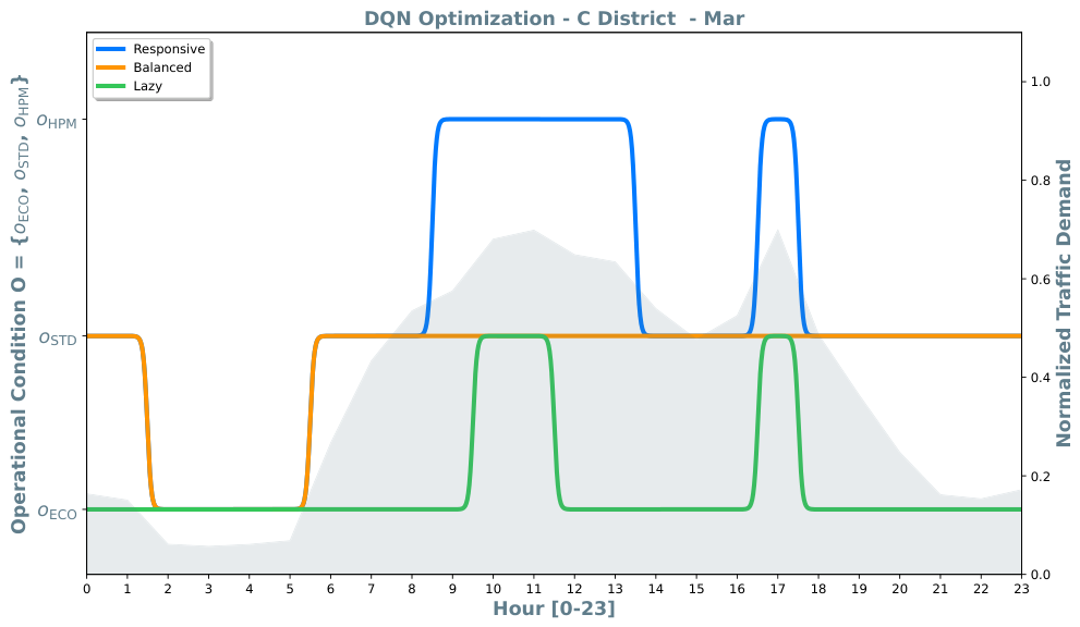
In the March scenario depicted in Figure 11, the analysis confirms the characteristic behavior of the three policies. The lazy policy maintains devices in $o_{ECO}$, activating the $o_{STD}$ condition only during peaks in demand (around 11:00 and 17:00). The balanced policy maintains its cost-oriented objective. Finally, the responsive policy confirms its high sensitivity.

The cross-seasonal analysis confirms that the DQN agent has successfully synthesized three distinct optimization policies. The policy convergence observed across the four representative months suggests a high degree of robustness: regardless of the seasonal baseline, the lazy policy consistently acts as a lower bound for energy expenditure, while the responsive policy serves as a high-fidelity upper bound, with a direct benefit in terms of social sustainability.

The balanced policy exhibits an intermediate and stabilizing behavior. It effectively filters out minor traffic fluctuations to maintain devices in a steady $o_{STD}$ monitoring state, proving to be a compromise profile between social, economic, and environmental sustainability, without incurring the economic penalties of the responsive mode. However, the balanced policy is weaker than the responsive one in addressing environmental sustainability.

The empirical values and associated percentage markers reported in

Table 11. Edge-computed quantitative breakdown of policy–demand mismatch (${\mathcal{I}}_p$), under-provisioning stress (${\mathcal{I}}_p^{-}$), and over-provisioning waste (${\mathcal{I}}_p^{+}$) across seasonal scenarios.

Seasonal Scenario	Policy	Total Mismatch (${\mathcal{I}}_{\mathit{p}}$)	Under-Prov. (${\mathcal{I}}_{\mathit{p}}^{-}$)	Over-Prov. (${\mathcal{I}}_{\mathit{p}}^{+}$)
August	${\pi }_l$	5.40 ($22.5\%$)	4.30 ($17.9\%$)	1.10 ($4.6\%$)
(Summer Peak)	${\pi }_b$	3.10 ($12.9\%$)	0.90 ($3.8\%$)	2.20 ($9.1\%$)
	${\pi }_r$	4.80 ($20.0\%$)	0.10 ($0.4\%$)	4.70 ($19.6\%$)
October	${\pi }_l$	5.85 ($24.4\%$)	4.95 ($20.6\%$)	0.90 ($3.8\%$)
(Autumn Routine)	${\pi }_b$	2.65 ($11.0\%$)	0.75 ($3.1\%$)	1.90 ($7.9\%$)
	${\pi }_r$	5.15 ($21.5\%$)	0.15 ($0.6\%$)	5.00 ($20.9\%$)
January	${\pi }_l$	5.10 ($21.3\%$)	4.50 ($18.8\%$)	0.60 ($2.5\%$)
(Winter Drop)	${\pi }_b$	2.35 ($9.8\%$)	0.85 ($3.5\%$)	1.50 ($6.3\%$)
	${\pi }_r$	5.90 ($24.6\%$)	0.20 ($0.8\%$)	5.70 ($23.8\%$)
March	${\pi }_l$	5.65 ($23.5\%$)	4.85 ($20.2\%$)	0.80 ($3.3\%$)
(Spring Surge)	${\pi }_b$	2.45 ($10.2\%$)	0.70 ($2.9\%$)	1.75 ($7.3\%$)
	${\pi }_r$	4.95 ($20.6\%$)	0.15 ($0.6\%$)	4.80 ($20.0\%$)

provide a quantitative proof, mapping the operational trade-offs in all seasonal variations. The indicators of daily mismatch are computed as ${\mathcal{I}}_p={\mathcal{I}}_p^{-}+{\mathcal{I}}_p^{+}$, where the total error ${\mathcal{I}}_p={\sum }_{t=0}^{23}|{\mathsf{\Pi }}_p\left(t\right)-D\left(t\right)|$ is broken down into under-production stress ${\mathcal{I}}_p^{-}={\sum }_{t=0}^{23}\max (0,D\left(t\right)-{\mathsf{\Pi }}_p\left(t\right))$ and over-production waste ${\mathcal{I}}_p^{+}={\sum }_{t=0}^{23}\max (0,{\mathsf{\Pi }}_p\left(t\right)-D\left(t\right))$, normalized relative to a maximum theoretical daily horizon of 24 h.

The lazy policy (${\pi }_l$) registers the highest under-provisioning stress, accumulating a daily deficit that peaks at $4.95$ ($20.6\%$) in October and reaches $4.85$ ($20.2\%$) in March. By locking the infrastructure into low-power execution during high-traffic periods, this policy triggers an information blackout. This degradation is most evident during the diurnal period: the gap against the traffic demand profile induces a localized under-provisioning spike of up to $40\%$, averaging a data loss of over $28\%$ during commuter hours. The system flags this communication gap as a critical environmental multiplier; losing real-time edge telemetry collapses parking optimization algorithms, severely increasing vehicular cruising times and indirect urban emissions.

Conversely, the responsive policy (${\pi }_r$) minimizes under-provisioning to a negligible margin between $0.10$ ($0.4\%$) and $0.20$ ($0.8\%$), guaranteeing city-wide traffic mitigation by absorbing sudden demand peaks. However, this operational safety comes at the expense of over-provisioning waste. Specifically, ${\mathcal{I}}_p^{+}$ reaches up to $5.70$ ($23.8\%$) in January, periodically trapping the network nodes in maximum power dissipation.

Bridging this gap, the balanced policy (${\pi }_b$) systematically scores the lowest total mismatch (${\mathcal{I}}_p$) across all seasons, achieving an optimal low of $2.35$ ($9.8\%$) in January and bounding the daily deviation within a tight 10.2–12.9% window.

To establish a rigorous cross-layer evaluation of the proposed framework, it is critical to formalize the operational baseline prior to the deployment of the DQN agent. Initially, the framework processes raw seasonal and traffic datasets collected directly from the monitored urban testbed. These data streams, which capture the physical city dynamics under traditional management (i.e., without optimization), are normalized and serve as the static empirical baseline (graphically represented as the shaded gray reference profiles in Figure 8, Figure 9, Figure 10 and Figure 11).

Under the proposed framework, when the DQN agent is activated, it evaluates this baseline to dynamically trigger one of the three policies (${\pi }_l$, ${\pi }_b$, ${\pi }_r$) across the operational conditions $O=\{o_{ECO},o_{STD},o_{HPM}\}$. The deployment of a specific policy $\pi$ inherently triggers a closed-loop feedback mechanism that modifies the environment itself. To capture this cross-layer dependency, the physical traffic demand evolution for the subsequent operational interval is modeled by Equation (27) [23,63]:

$$V_{t+1}\left({\mathcal{I}}_{p,t}^{-}\right)=V_{t,\mathrm{base}}·\left(1+\mu ·{\mathcal{I}}_{p,t}^{-}\right)$$

(27)

where $V_{t+1}\left({\mathcal{I}}_{p,t}^{-}\right)$ represents the predicted dynamic traffic volume demand at time interval $t+1$, formalizing how the environmental baseline shifts as a direct consequence of the telemetry policy applied at time t; $V_{t,\mathrm{base}}$ is the unoptimized baseline (datasets) for the current time interval t; ${\mathcal{I}}_{p,t}^{-}$ represents the under-provisioning stress computed at time t (as compiled in Table 11); and $\mu$ is the urban multiplier within the bounded sensitivity range $\mu \in [1.0,3.0]$. A value of $\mu =1.0$ represents the fundamental, unamplified baseline; higher values (up to $\mu =3.0$) model a highly sensitive collapse scenario, capturing how transient data gaps cascade into macro-urban gridlocks when the transportation network approaches critical saturation.

Conversely, the over-provisioning stress (${\mathcal{I}}_{p,t}^{+}$) formalizes the unnecessary active radio states maintained above the dataset’s demand curve, directly driving up hardware power consumption and infrastructure operational expenditure (${\mathrm{OPEX}}_{\inf }$).

To evaluate the resilience of the proposed framework against different urban dynamics, a comprehensive cross-layer sensitivity analysis was performed by varying the urban amplification multiplier $\mu$ from $1.0$ up to $3.0$. As shown in

Table 12. Cross-layer sensitivity analysis: Predictive quantification of traffic inflation ($\Delta V_{t+1}$) across multiple $\mu$ horizons relative to invariant infrastructure KPIs (${\eta }_E$, PDR).

		Invariant KPIs		Predicted Traffic Inflation ($\mathbf{\Delta }{\mathit{V}}_{\mathit{t}+1}$)
Scenario	Policy	Net Energy	Network	$\mathit{\mu }\mathbf{=}\mathbf{1.0}$	$\mathit{\mu }\mathbf{=}\mathbf{1.5}$	$\mathit{\mu }\mathbf{=}\mathbf{2.0}$	$\mathit{\mu }\mathbf{=}\mathbf{2.5}$	$\mathit{\mu }\mathbf{=}\mathbf{3.0}$
		Saving (${\mathbf{\eta }}_{\mathbf{E}}$)	PDR	(Linear)	(Base)	(High)	(Severe)	(Limit)
August	${\pi }_l$	+15.0%	82.1%	+17.9%	+26.8%	+35.8%	+44.8%	+53.7%
	${\pi }_b$	+10.5%	96.2%	+3.8%	+5.7%	+7.6%	+9.5%	+11.4%
	${\pi }_r$	0.0% (Base)	99.6%	+0.4%	+0.6%	+0.8%	+1.0%	+1.2%
October	${\pi }_l$	+17.1%	79.4%	+20.6%	+30.9%	+41.2%	+51.5%	+61.8%
	${\pi }_b$	+13.0%	96.9%	+3.1%	+4.6%	+6.2%	+7.8%	+9.3%
	${\pi }_r$	0.0% (Base)	99.4%	+0.6%	+0.9%	+1.2%	+1.5%	+1.8%
January	${\pi }_l$	+21.3%	81.2%	+18.8%	+28.2%	+37.6%	+47.0%	+56.4%
	${\pi }_b$	+17.5%	96.5%	+3.5%	+5.2%	+7.0%	+8.8%	+10.5%
	${\pi }_r$	0.0% (Base)	99.2%	+0.8%	+1.2%	+1.6%	+2.0%	+2.4%
March	${\pi }_l$	+16.7%	79.8%	+20.2%	+30.3%	+40.4%	+50.5%	+60.6%
	${\pi }_b$	+12.7%	97.1%	+2.9%	+4.3%	+5.8%	+7.3%	+8.7%
	${\pi }_r$	0.0% (Base)	99.4%	+0.6%	+0.9%	+1.2%	+1.5%	+1.8%

, the CPS infrastructure metrics, namely, net energy savings (${\eta }_E$) and the network $PDR$, are invariant across all $\mu$ horizons: the sensors work in their own operating modes, switching between $ECO$, $STD$, and $HPM$, but the physical traffic conditions do not change how these sensors behave.

Conversely, the physical traffic inflation ($\Delta V_{t+1}$) scales proportionally with $\mu$, explicitly revealing the operational risks associated with uncoordinated sensor sleep-scheduling. Under the lazy policy (${\pi }_l$), the data gaps induced to maximize energy savings trigger a severe traffic accumulation penalty. This penalty escalates from a manageable $+20.6\%$ under a linear topology ($\mu =1.0$) to an unsustainable $+61.8\%$ under heavy gridlock conditions ($\mu =3.0$) during peak commuter months such as October.

Crucially, the balanced policy (${\pi }_b$) mitigates this cross-layer degradation. Even under the most conservative and non-linear urban scenario ($\mu =3.0$), ${\pi }_b$ restricts the maximum traffic inflation to just $+11.4\%$ in August and $+9.3\%$ in October, while simultaneously preserving significant net energy savings of up to $+17.5\%$ (January). These findings prove the capability of the framework under ${\pi }_b$ to maintain stable urban mobility indicators across highly diverse physical infrastructures without requiring local hardware recalibration.

The environmental efficacy of the proposed framework is mathematically quantified by translating macroscopic traffic anomalies into a standardized ecological metric. We define the Net Carbon-Emission Reduction Rate (${\eta }_{C{O}_2}$) for a generic policy $\pi$ under a specific urban stress level $\mu$ as the relative percentage of avoided excess vehicular greenhouse gas emissions, formally defined by Equation (28) [23]:

$${\eta }_{C{O}_2}{\left(\pi \right)|}_{\mu }={\displaystyle \frac{\Delta V_{t+1}\left({\pi }_l\right){{|}_{\mu }-\Delta V_{t+1}\left(\pi \right)|}_{\mu }}{\Delta V_{t+1}\left({\pi }_l\right){|}_{\mu }}}$$

(28)

where $\Delta V_{t+1}{\left(\pi \right)|}_{\mu }$ represents the predicted traffic inflation under policy $\pi$ and stress $\mu$. The lazy policy (${\pi }_l$) is assumed as the worst-case environmental baseline ($0.0\%$ mitigation reference).

Results are shown in

Table 13. Cross-layer environmental sensitivity analysis: Quantitative Carbon-Emission Reduction Rate (${\eta }_{C{O}_2}$) and predicted traffic mitigation across multiple urban stress horizons ($\mu$).

		Hardware State	Carbon-Emission Reduction Rate (${\mathit{\eta }}_{{\mathbf{CO}}_2}$) vs. Lazy Baseline
Scenario	Policy	Profile (Ref)	$\mathit{\mu }\mathbf{=}\mathbf{1.0}$	$\mathit{\mu }\mathbf{=}\mathbf{1.5}$	$\mathit{\mu }\mathbf{=}\mathbf{2.0}$	$\mathit{\mu }\mathbf{=}\mathbf{2.5}$	$\mathit{\mu }\mathbf{=}\mathbf{3.0}$
		(Energy/PDR)	(Linear)	(Base)	(High)	(Severe)	(Limit)
August	${\pi }_l$	+15.0%/82.1%	0.0% (Base)	0.0% (Base)	0.0% (Base)	0.0% (Base)	0.0% (Base)
	${\pi }_b$	+10.5%/96.2%	78.77%	78.73%	78.77%	78.79%	78.77%
	${\pi }_r$	0.0%/99.6%	97.77%	97.76%	97.77%	97.77%	97.77%
October	${\pi }_l$	+17.1%/79.4%	0.0% (Base)	0.0% (Base)	0.0% (Base)	0.0% (Base)	0.0% (Base)
	${\pi }_b$	+13.0%/96.9%	84.95%	85.11%	84.95%	84.85%	84.95%
	${\pi }_r$	0.0%/99.4%	97.09%	97.09%	97.09%	97.09%	97.09%
January	${\pi }_l$	+21.3%/81.2%	0.0% (Base)	0.0% (Base)	0.0% (Base)	0.0% (Base)	0.0% (Base)
	${\pi }_b$	+17.5%/96.5%	81.38%	81.56%	81.38%	81.28%	81.38%
	${\pi }_r$	0.0%/99.2%	95.74%	95.74%	95.74%	95.74%	95.74%
March	${\pi }_l$	+16.7%/79.8%	0.0% (Base)	0.0% (Base)	0.0% (Base)	0.0% (Base)	0.0% (Base)
	${\pi }_b$	+12.7%/97.1%	85.64%	85.81%	85.64%	85.54%	85.64%
	${\pi }_r$	0.0%/99.4%	97.03%	97.03%	97.03%	97.03%	97.03%

. The responsive policy (${\pi }_r$) consistently delivers the absolute highest ecological benefit across all seasonal horizons and urban stress scales, exhibiting a clear structural advantage over both the lazy (${\pi }_l$) and balanced (${\pi }_b$) approaches.

For instance, during the critical winter peak in January under severe stress ($\mu =2.5$), the balanced policy (${\pi }_b$) mitigates $81.28\%$ of excess emissions, whereas the responsive policy (${\pi }_r$) reaches a massive emission reduction rate of $95.74\%$.

Similarly, in the October scenario, ${\pi }_r$ dynamically secures a steady and uniform $97.09\%$ drop in excess vehicular emissions across all evaluated $\mu$ values (e.g., preventing the $+61.8\%$ traffic inflation of ${\pi }_l$ at $\mu =3.0$ by restricting it to just $+1.8\%$). These empirical outcomes demonstrate that while ${\pi }_r$ entirely sacrifices local infrastructure energy savings (${\eta }_E=0.0\%$), it achieves an optimal cross-layer trade-off, showing that a minor energy investment at the edge network layer yields a massive, systemic containment of urban air pollution and structural transport gridlocks.

4.1. TCO Analysis

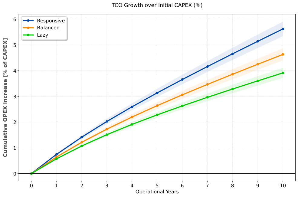
The economic sustainability of the examined CPS is evaluated through a $TCO$ analysis over a 10-year operational horizon. The initial $CAPEX$ is established as the baseline and comprises the acquisition of the equipment shown in Table 6, alongside a centralized gateway, software orchestration platforms, and professional installation costs. The growth in $TCO$ is driven by the $OPEX$, and it is primarily conditioned by energy consumption costs, assuming a baseline rate of $0.20€/\mathrm{kWh}$, and system maintenance costs.

The results in Figure 12 allow an investigation of the policy sensitivity: the responsive policy exhibits higher growth, reaching an OPEX-to-CAPEX ratio of approximately $5.6$% after 10 years. The DQN agent consistently prioritizes the $o_{HPM}$ mode to ensure near-zero latency and high information fidelity during peak traffic demand, which inherently maximizes the power draw across the NVIDIA Jetson Nano rails.

The lazy policy achieves the highest economic sustainability, limiting the 10-year $OPEX$ increase to less than 4%. All policies show a subtle transition to a linear trend after the initial five-year phase, reflecting their stabilization and leading to a predictable marginal cost per year.

Finally, the balanced policy shows a mid-range trade-off. These savings are achieved with 95% confidence intervals, ensuring the reliability of the economic projections.

4.2. Trade-Off Alignment with UN SDG 11 Targets

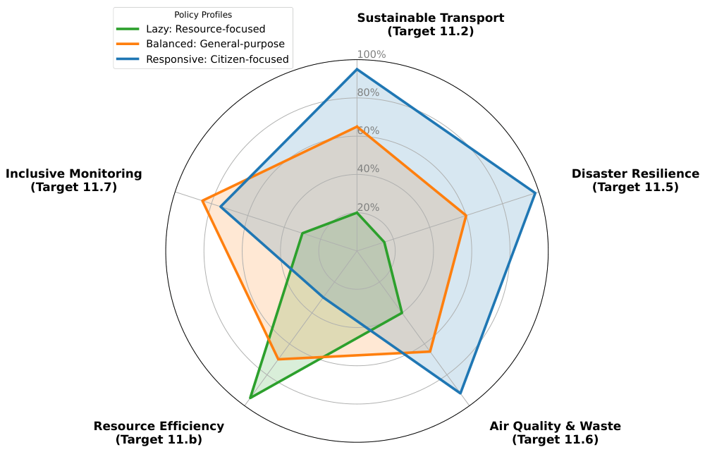
The radar plot in Figure 13 maps the profiles of the implemented policies on a set of UN SDG 11 targets. This map is obtained considering the set of heterogeneous metrics of the dynamic urban context $C\left(t\right)$ defined in Equation (25).

The responsive policy shows a clear prioritization of Target 11.2 (Sustainable Transport) and Target 11.5 (Disaster Resilience and Safety). By proactively escalating to the high-performance state $o_{HPM}$ during traffic peaks, the agent ensures the fidelity of the information required to mitigate congestion and reduce emergency response times. This citizen-centric behavior acknowledges that a localized increase in energy consumption $E(s,t)$ is a strategic investment to achieve systemic environmental benefits and public safety, directly supporting Target 11.6 (Reducing the Environmental Impact of Cities).

Conversely, the lazy policy aligns primarily with Target 11.b (Resource Efficiency). By maintaining the infrastructure in a low-power $o_{ECO}$ state for the majority of the operational cycle, it minimizes the carbon footprint $CF(s,t)$ and the operational expenditure $OPEX$. While this approach maximizes the physical and financial longevity of the CPS, it results in lower performance regarding real-time mobility management.

Finally, the balanced policy identifies an equilibrium point for Target 11.7 (Inclusive and Reliable Monitoring). By acting as a stable baseline in $o_{STD}$, it provides continuous and reliable data flows without the energy surges of the responsive mode or the data scarcity of the lazy profile.

The analysis confirms that the DQN-based framework does not merely optimize a technical trade-off but offers an optimal set of strategies. This allows municipal decision-makers to dynamically tune the infrastructure behavior to meet specific sustainability priorities, from strict resource conservation to high-fidelity urban resilience.

4.3. Threats to Validity

In this section, we critically discuss the potential threats to the validity of our study, categorized into internal, external, and construct validity, along with the mitigation strategies adopted.

4.3.1. Internal Validity

Internal validity concerns internal factors or hidden assumptions that might have influenced the experimental results.

The comparative analysis presented in this study primarily focuses on the three internal operational policies ($\pi$) in Equation (21), namely, lazy, balanced, and responsive, which are synthesized by manipulating the weight coefficients ($\lambda$) within the multi-objective reward function in Equation (20). A limitation of our study is the absence of a separate, external algorithm to test against. To mitigate this threat, we designed our policies to directly replicate the three standard rule-based configurations currently used in legacy smart city gateways. These settings serve as our control groups, representing traditional static management focused on either extreme energy savings, a fixed compromise, or high responsiveness. Our analysis demonstrates that a single DQN engine can dynamically adapt to all three conflicting targets, whereas traditional networks require rigid, manual hardware reconfiguration. Testing against external metaheuristics remains a key objective for future work.

4.3.2. External Validity

External validity relates to the generalization of our findings to other scenarios or real-world platforms.

Our long-term TCO projections, presented in Figure 12, are the result of a baseline structural model derived from nominal vendor component pricing, standardized hardware lifespans, and fixed electricity tariffs. In a real smart city deployment, empirical TCO curves are inherently non-linear and subject to volatile fluctuations. These economic variations are driven by real-world stochastic factors, including localized maintenance labor spikes, equipment replacement cycles, severe weather interventions, cloud-service fee restructuring, software maintenance, inflation, and electricity-price volatility, alongside physical constraints like sensor aging and battery degradation.

To mitigate this threat to validity, our economic evaluation must be interpreted as an expected mathematical baseline, representing the long-term structural cost trend, around which real-world operational expenditures will inevitably oscillate. Crucially, these real-world perturbations do not invalidate the comparative economic advantages demonstrated by our framework: by dynamically minimizing the operational resource and transmission overhead at the edge, the proposed DQN model actively compresses the baseline energy footprint and mitigates hardware stress. Consequently, it provides the physical network infrastructure with a more resilient buffer against external electricity-price fluctuations and reduces the frequency of premature equipment replacements caused by sensor and node degradation.

4.3.3. Construct Validity

Construct validity assesses whether our performance metrics accurately reflect the higher-level goals of the study.

Pure networking performance, such as that based on PDR and latency, does not inherently equate to social dimensions such as equity, accessibility, or public participation. To mitigate this conceptual threat, the framework strictly treats QoS not as a direct measure of social sustainability but as a critical technological enabler (or proxy) for public service quality. Under UN SDG 11, high network responsiveness and data reliability are fundamental prerequisites for deploying dependable disaster early-warning systems (SDG 11.5) and real-time environmental hazard monitoring (SDG 11.6). Without a guaranteed QoS baseline, these public services fail, impacting vulnerable urban groups. While our current evaluation is limited to these technical proxies, including explicit social indicators, such as public feedback loops, accessibility metrics, and user privacy constraints, will be an upgrade for future work to fully validate the social pillar of the framework.

5. Conclusions and Future Directions

The proposed multi-dimensional decision-making framework successfully transitions urban management from static, siloed ICT deployments to an integrated, adaptive urban Cyber–Physical System. By leveraging Deep Reinforcement Learning, specifically Deep Q-Networks, the model effectively navigates the non-linear trade-offs inherent in the environmental, economic, and social pillars of sustainability. The presented methodology mitigates the inefficiencies of traditional high-performance configurations while preserving the resilience required for modern urban infrastructures. The empirical results from the LoRaWAN case study demonstrate the practical effectiveness and validation of the framework. This research confirms that the intersection of autonomous AI agents and granular urban telemetry is essential for fulfilling the complex requirements of UN Sustainable Development Goal 11. The potential threats to the validity of our study have been discussed and categorized into internal, external, and construct validity, along with the mitigation strategies adopted.

Future iterations of this work will focus on testing the architectural portability of the DQN loop across diverse municipal topologies and heterogeneous communication standards. Moreover, we will explore the integration of decentralized federated learning to further enhance data privacy and system-wide scalability in heterogeneous urban environments. To address long-term challenges, aging-/reliability-aware frameworks are envisioned to be integrated into the DQN controller. A feasible way to achieve this is to introduce a cumulative stress counter as a state variable, allowing the agent to learn to proactively mitigate hardware aging.

References

1. Alahi, M.E.E.; Sukkuea, A.; Tina, F.W.; Nag, A.; Kurdthongmee, W.; Suwannarat, K.; Mukhopadhyay, S.C. Integration of IoT-Enabled Technologies and Artificial Intelligence (AI) for Smart City Scenario: Recent Advancements and Future Trends. Sensors 2023, 23, 5206. [Google Scholar] [CrossRef]
2. Bellini, P.; Nesi, P.; Pantaleo, G. IoT-Enabled Smart Cities: A Review of Concepts, Frameworks and Key Technologies. Appl. Sci. 2022, 12, 1607. [Google Scholar] [CrossRef]
3. United Nations. Sustainable Development Goals. Department of Economic and Social Affairs. Available online: https://sdgs.un.org/goals (accessed on 30 March 2026).
4. Bittencourt, J.C.N.; Jesus, T.C.; Peixoto, J.P.J.; Costa, D.G. The Road to Intelligent Cities. Smart Cities 2025, 8, 77. [Google Scholar] [CrossRef]
5. Zghidi, N.; Trabelsi, R. Impact of Digitalization on Sustainable Development: A Comparative Analysis of Developed and Developing Economies. J. Risk Financ. Manag. 2025, 18, 359. [Google Scholar] [CrossRef]
6. Wang, K.; Ke, Y. Social sustainability of communities: A systematic literature review. Sustain. Prod. Consum. 2024, 47, 585–597. [Google Scholar] [CrossRef]
7. Capecchi, S.; Corduas, M.; Piccolo, D. Social Sustainability and Subjective Well-Being: A Study on Italian Inner Areas. Sustainability 2025, 17, 2078. [Google Scholar] [CrossRef]
8. Minskere, L.; Kalnina, D.; Salkovska, J.; Batraga, A. Urban Communication in Smart Cities: Stakeholder Participation Motivators. Smart Cities 2026, 9, 58. [Google Scholar] [CrossRef]
9. Seng, K.P.; Ang, L.M.; Ngharamike, E. Artificial intelligence Internet of Things: A new paradigm of distributed sensor networks. Int. J. Distrib. Sens. Netw. 2022, 18, 15501477211062835. [Google Scholar] [CrossRef]
10. Pochelu, P.; Cartiaux, H.; Schleich, J. What artificial intelligence can do for high-performance computing systems? Eng. Appl. Artif. Intell. 2026, 164, 113248. [Google Scholar] [CrossRef]
11. Bibri, S.E.; Huang, J. Artificial intelligence of things for sustainable smart city brain and digital twin systems: Pioneering environmental synergies between real-time management and predictive planning. Environ. Sci. Ecotechnol. 2025, 26, 100591. [Google Scholar] [CrossRef]
12. Das, D.K.; Aiyetan, A.O.; Mostafa, M.M.H. Advancing Smart Cities in Africa: Barriers, Potentials, and Strategic Pathways for Sustainable Urban Transformation. Smart Cities 2026, 9, 38. [Google Scholar] [CrossRef]
13. Abu-Rayash, A.; Dincer, I. Development of an integrated model for environmentally and economically sustainable and smart cities. Sustain. Energy Technol. Assess. 2025, 73, 104096. [Google Scholar] [CrossRef]
14. Shafiullah, M.; Katranji, A.R.; Hassan, M.; Rahman, M.M.; Shezan, S.A. Advanced Multivariate Deep Learning Methodology for Forecasting Wind Speed and Solar Irradiation. Smart Cities 2026, 9, 59. [Google Scholar] [CrossRef]
15. Santos, O.; Ribeiro, F.; Metrôlho, J.; Dionísio, R. Using Smart Traffic Lights to Reduce CO2 Emissions and Improve Traffic Flow at Intersections: Simulation of an Intersection in a Small Portuguese City. Appl. Syst. Innov. 2024, 7, 3. [Google Scholar] [CrossRef]
16. Bisegna, F.; Vespasiano, F.; Pompei, L.; Burattini, C.; Belli, E.; Bellucci, A.M.; Di Vittorio, F.; Blaso, L. Towards the Decarbonization of Urban Communities: Evaluation of Smart and Green Strategies to Reduce Gas Carbon Emissions. Smart Cities 2026, 9, 26. [Google Scholar] [CrossRef]
17. Mekki, K.; Bajic, E.; Chaxel, F.; Meyer, F. A comparative study of LPWAN technologies for large-scale IoT deployment. ICT Express 2019, 5, 1–7. [Google Scholar] [CrossRef]
18. Giacobbe, M.; Zanafi, S.; Zaia, A.; Puliafito, A. Empirical Validation of LoRaWAN Coverage Models for Smart Urban Connectivity. In Proceedings of the 39th ECMS International Conference on Modelling and Simulation, ECMS 2025, Catania, Italy, 24–27 June 2025; Volume 493, p. 499. [Google Scholar] [CrossRef]
19. Terven, J. Deep Reinforcement Learning: A Chronological Overview and Methods. AI 2025, 6, 46. [Google Scholar] [CrossRef]
20. Plaat, A. Deep Reinforcement Learning; Springer Nature Singapore: Singapore, 2022; ISBN 978-981-19-0638-1. [Google Scholar] [CrossRef]
21. Kim, S.-K.; Chan, I.C. Novel Machine Learning-Based Smart City Pedestrian Road Crossing Alerts. Smart Cities 2025, 8, 114. [Google Scholar] [CrossRef]
22. Palley, B.; Poças Martins, J.; Bernardo, H.; Rossetti, R. Integrating Machine Learning and Digital Twins for Enhanced Smart Building Operation and Energy Management: A Systematic Review. Urban Sci. 2025, 9, 202. [Google Scholar] [CrossRef]
23. Sutton, R.S.; Barto, A.G. Reinforcement learning. J. Cogn. Neurosci. 1999, 11, 126–134. [Google Scholar] [CrossRef]
24. Oh, J.; Farquhar, G.; Kemaev, I.; Calian, D.A.; Hessel, M.; Zintgraf, L.; Singh, S.; van Hasselt, H.; Silver, D. Discovering state-of-the-art reinforcement learning algorithms. Nature 2025, 648, 312–319. [Google Scholar] [CrossRef]
25. Remmache, M.I.; Boudouh, S.S.; Bendouma, T.; Abdelhafidi, Z. Balancing Energy and Latency in Multi-Edge MEC Systems Using DQN-Based Task Offloading. In Proceedings of the 2025 7th International Conference on Pattern Analysis and Intelligent Systems (PAIS), Laghouat, Algeria, 23–24 April 2025; pp. 1–5. [Google Scholar] [CrossRef]
26. Liang, J.; Miao, H.; Li, K.; Tan, J.; Wang, X.; Luo, R.; Jiang, Y. A Review of Multi-Agent Reinforcement Learning Algorithms. Electronics 2025, 14, 820. [Google Scholar] [CrossRef]
27. Hady, M.A.; Hu, S.; Pratama, M.; Cao, Z.; Kowalczyk, R. Multi-agent reinforcement learning for resources allocation optimization: A survey. Artif. Intell. Rev. 2025, 58, 354. [Google Scholar] [CrossRef]
28. Dong, P.; Tao, H.; Luo, H.; Shi, W.; Wang, J.; Zhou, J. MACS: LLM-Enhanced Multi-AUV Collaborative Search Scheme via Multi-agent Reinforcement Learning. IEEE Internet Things J. 2026, 13, 27197–27213. [Google Scholar] [CrossRef]
29. Fatorachian, H.; Kazemi, H.; Pawar, K. Digital Technologies in Food Supply Chain Waste Management: A Case Study on Sustainable Practices in Smart Cities. Sustainability 2025, 17, 1996. [Google Scholar] [CrossRef]
30. Fatorachian, H.; Kazemi, H.; Pawar, K. Enhancing Smart City Logistics Through IoT-Enabled Predictive Analytics: A Digital Twin and Cybernetic Feedback Approach. Smart Cities 2025, 8, 56. [Google Scholar] [CrossRef]
31. De Vita, F.; Nardini, G.; Virdis, A.; Bruneo, D.; Puliafito, A.; Stea, G. Using Deep Reinforcement Learning for Application Relocation in Multi-Access Edge Computing. IEEE Commun. Stand. Mag. 2019, 3, 71–78. [Google Scholar] [CrossRef]
32. Ficili, I.; Giacobbe, M.; Tricomi, G.; Puliafito, A. From Sensors to Data Intelligence: Leveraging IoT, Cloud, and Edge Computing with AI. Sensors 2025, 25, 1763. [Google Scholar] [CrossRef]
33. De Vita, F.; Bruneo, D. Leveraging Stack4Things for Federated Learning in Intelligent Cyber Physical Systems. J. Sens. Actuator Netw. 2020, 9, 59. [Google Scholar] [CrossRef]
34. Chen, M.; Sun, L.; Li, T.; Sun, H.; Zhou, Y.; Zhu, C.; Wang, H.; Pan, J.Z.; Zhang, W.; Chen, H.; et al. ReSearch: Learning to Reason with Search for LLMs via Reinforcement Learning. arXiv 2025. [Google Scholar] [CrossRef]
35. Hubert, T.; Mehta, R.; Sartran, L.; Horváth, M.Z.; Žužić, G.; Wieser, E.; Huang, A.; Schrittwieser, J.; Schroecker, Y.; Masoom, H.; et al. Olympiad-level formal mathematical reasoning with reinforcement learning. Nature 2026, 651, 607–613. [Google Scholar] [CrossRef]
36. Liu, R.; Nageotte, F.; Zanne, P.; de Mathelin, M.; Dresp-Langley, B. Deep Reinforcement Learning for the Control of Robotic Manipulation: A Focussed Mini-Review. Robotics 2021, 10, 22. [Google Scholar] [CrossRef]
37. Beguni, C.; Căilean, A.-M.; Zadobrischi, E.; Avătămăniței, S.-A.; Lavric, A.; Stoian, F.-M. The Convergence of Artificial Intelligence and Public Policy in Shaping the Future of Ride-Hailing: A Review. Smart Cities 2026, 9, 40. [Google Scholar] [CrossRef]
38. Chaudhari, S.; Aggarwal, P.; Murahari, V.; Rajpurohit, T.; Kalyan, A.; Narasimhan, K.; Deshpande, A.; da Silva, B.C. RLHF Deciphered: A Critical Analysis of Reinforcement Learning from Human Feedback for LLMs. ACM Comput. Surv. 2025, 58, 53. [Google Scholar] [CrossRef]
39. Kim, Y.; Jung, B.C.; Song, Y. Online Learning for Joint Energy Harvesting and Information Decoding Optimization in IoT-Enabled Smart City. IEEE Internet Things J. 2023, 10, 10675–10686. [Google Scholar] [CrossRef]
40. Zhang, B.; Liu, C.H.; Tang, J.; Xu, Z.; Ma, J.; Wang, W. Learning-Based Energy-Efficient Data Collection by Unmanned Vehicles in Smart Cities. IEEE Trans. Ind. Inform. 2018, 14, 1666–1676. [Google Scholar] [CrossRef]
41. Park, J.; Baek, J.; Song, Y. Optimizing smart city planning: A deep reinforcement learning framework. ICT Express 2025, 11, 129–134. [Google Scholar] [CrossRef]
42. Alharbi, S. MORL-SGF: A Governance-Aware Multi-Objective Reinforcement Learning Framework with Digital Twin Policy Validation for Sustainable Smart Cities. Systems 2026, 14, 294. [Google Scholar] [CrossRef]
43. Sajid, S.; Li, B.; Qi, B.; Liang, F.; Lei, Y.; Muqtadir, A. Multi-Agent Reinforcement Learning for Demand Response in Grid-Responsive Buildings and Prosumer Communities: A PRISMA-Guided Systematic Review. Energies 2026, 19, 2170. [Google Scholar] [CrossRef]
44. Michailidis, P.; Michailidis, I.; Kosmatopoulos, E. Reinforcement Learning for Optimizing Renewable Energy Utilization in Buildings: A Review on Applications and Innovations. Energies 2025, 18, 1724. [Google Scholar] [CrossRef]
45. Mai, V.; Maisonneuve, P.; Zhang, T.; Nekoei, H.; Paull, L.; Lesage-Landry, A. Multi-agent reinforcement learning for fast-timescale demand response of residential loads. Mach. Learn. 2024, 113, 5203–5234. [Google Scholar] [CrossRef]
46. Agarwal, T.; Arora, H.; Schneider, J. Learning Urban Driving Policies using Deep Reinforcement Learning. In Proceedings of the 2021 IEEE International Intelligent Transportation Systems Conference (ITSC), Indianapolis, IN, USA, 19–22 September 2021; pp. 607–614. [Google Scholar] [CrossRef]
47. Li, Q.; Peng, B.; Li, Q.; Lin, M.; Chen, C.; Peng, S. A Latency-Optimal Task Offloading Scheme Using Genetic Algorithm for DAG Applications in Edge Computing. In Proceedings of the 2023 8th International Conference on Cloud Computing and Big Data Analytics (ICCCBDA), Chengdu, China, 26–28 April 2023; pp. 344–348. [Google Scholar] [CrossRef]
48. Molokomme, D.N.; Onumanyi, A.J.; Abu-Mahfouz, A.M. An Emulated Dynamic Framework for Evaluating Metaheuristic-Based Load Balancing Techniques in Edge Computing Networks. AI 2026, 7, 81. [Google Scholar] [CrossRef]
49. Jyoti, K.S.; Gokuldhev, M. A probabilistic genetic algorithm approach to efficient task scheduling in cloud-edge environments. CLEI Electron. J. 2026, 28. [Google Scholar] [CrossRef]
50. Chen, X.; Zhang, J.; Lin, B.; Chen, Z.; Wolter, K.; Min, G. Energy-Efficient Offloading for DNN-Based Smart IoT Systems in Cloud-Edge Environments. IEEE Trans. Parallel Distrib. Syst. 2022, 33, 683–697. [Google Scholar] [CrossRef]
51. Hu, X.-M.; Zhan, Z.-H.; Lin, Y.; Gong, Y.-J.; Yu, W.-J.; Hu, Y.-X. Multiobjective genetic algorithm for demand side management of smart grid. In Proceedings of the 2013 IEEE Symposium on Computational Intelligence in Scheduling (CISched), Singapore, 16–19 April 2013; pp. 14–21. [Google Scholar] [CrossRef]
52. Mousavi-Ghasemlou, S.; Ochoa-Zezzatti, A.; Zapotecas-Martínez, S.; Oliva, D.; Lira, M.; Garcia-Villalba, L.A. Sustainable Energy Management in Smart Cities: Optimizing Smart Grids Using Metaheuristic Algorithms. In Proceedings of the 2026 IEEE Conference on Artificial Intelligence (CAI), Granada, Spain, 8–10 May 2026; pp. 535–540. [Google Scholar] [CrossRef]
53. Odeh, S.; Hazboun, S.; Ayyash, M.A. Congestion-Aware Genetic Algorithm for Urban Mobility Optimization in Intelligent Transportation Systems. In Proceedings of the 2026 1st International Conference on Emerging Technologies and Engineering Systems (ICETES), Amaan, Jordan, 7–9 April 2026; pp. 95–99. [Google Scholar] [CrossRef]
54. Bruneel, H. Analysis of a threshold-based priority queue. Queueing Syst. 2025, 109, 8. [Google Scholar] [CrossRef]
55. Fryganiotis, N.; Dimolitsas, I.; Stai, E.; Zafeiropoulos, A.; Papavassiliou, S. Model Predictive Control-Based Dynamic Resource Allocation: Enabler for Resilient Network Slicing. IEEE Netw. 2025, 39, 118–126. [Google Scholar] [CrossRef]
56. Eurostat. Smart Cities-Statistics on Urban Institutions, Statistics Explained. 2023. Available online: https://ec.europa.eu/eurostat/statistics-explained/SEPDF/cache/10719.pdf (accessed on 24 March 2026).
57. International Energy Agency (IEA). World Energy Outlook 2024; IEA Publications: Paris, France, 2024; Available online: https://www.iea.org/reports/world-energy-outlook-2024 (accessed on 24 March 2026).
58. ISO/IEC 25002:2024; Systems and Software Engineering—Software Product Quality Requirements and Evaluation (SQuaRE)—Managed Quality Model. ISO: Geneva, Switzerland, 2024.
59. Patterson, A.; Liao, V.; White, M. Robust Losses for Learning Value Functions. IEEE Trans. Pattern Anal. Mach. Intell. 2023, 45, 6157–6167. [Google Scholar] [CrossRef]
60. Zaitsev, D.A.; Shmeleva, T.R.; Ghaffari, P. Modeling Multidimensional Communication Lattices with Moore Neighborhood by Infinite Petri Nets. In Proceedings of the 2021 International Conference on Information and Digital Technologies (IDT), Zilina, Slovakia, 22–24 June 2021; pp. 171–181. [Google Scholar] [CrossRef]
61. LoRa Alliance. What Is LoRaWAN? 2026. Available online: https://lora-alliance.org/about-lorawan/ (accessed on 13 April 2026).
62. Phan, T.C.; Le, V.D.; Nguyen, T. Application of Dueling Double Deep Q-Network for Dynamic Traffic Signal Optimization: A Case Study in Danang City, Vietnam. Mach. Learn. Knowl. Extr. 2025, 7, 65. [Google Scholar] [CrossRef]
63. Zhu, S.; Zhao, Y.; Zhang, Y.; Li, Q.; Wang, W.; Yang, S. Short-Term Traffic Flow Prediction with Wavelet and Multi-Dimensional Taylor Network Model. IEEE Trans. Intell. Transp. Syst. 2021, 22, 3203–3208. [Google Scholar] [CrossRef]
Figure 1. United Nations Sustainable Cities and Communities Goal (SDG11) and its targets.
Smartcities 09 00117 g001
Figure 2. Conceptual framework of adaptive urban ecosystem composed of multiple AI-driven CPSs.
Smartcities 09 00117 g002
Figure 3. Overall architecture of the proposed multi-objective optimization framework leading to context-aware optimized urban trade-offs.
Smartcities 09 00117 g003
Figure 4. DQN-based optimization schema, highlighting the cyber-to-physical and physical-to-cyber transitions in the smart urban ecosystem.
Smartcities 09 00117 g004
Figure 5. Spatial 3 × 3 grid representation of the urban district forming the monitored urban center. The map is centered on the Moore-modeled district C(0,0), with radius r = 1 .
Smartcities 09 00117 g005
Figure 6. Comparative analysis of DQN training dynamics under different optimization criteria over 1000 episodes: (a) MSBE profile exhibiting high-frequency noise and sudden gradient shocks, and (b) smoothed, stable convergence profile achieved through Huber loss minimization.
Smartcities 09 00117 g006
Figure 7. Empirical phase-by-phase quantification of the absolute divergence ( | MSBE Huber | ).
Smartcities 09 00117 g007
Figure 8. DQN policy sensitivity analysis for the C district in August. The plot illustrates the trade-offs resulting from the DQN-based optimization relative to normalized traffic demand (shaded area).
Smartcities 09 00117 g008
Figure 9. DQN policy sensitivity analysis for the C district in October.
Smartcities 09 00117 g009
Figure 10. DQN policy sensitivity analysis for the C district in January.
Smartcities 09 00117 g010
Figure 11. DQN policy sensitivity analysis for the C district in March.
Smartcities 09 00117 g011
Figure 12. Expected structural long-term (10-year) TCO trends as a percentage of initial investment across different operational trade-offs. Results are reported with a 95% confidence interval (shadows).
Smartcities 09 00117 g012
Figure 13. DQN-based trade-off alignment with UN SDG 11 targets. The radar plot illustrates the alignment between the agent’s behavioral profiles and global indicators for sustainable and resilient cities.
Smartcities 09 00117 g013