Comparative Evaluation of Traffic Load Prediction Models for Intelligent Transportation Systems Using High-Resolution Urban Data

Highlights

What are the main findings?

• Comparative evaluation indicates that deep learning models show stronger capability in capturing complex temporal patterns under highly variable traffic conditions, while conventional models remain competitive during stable regimes.
• Prediction performance varies significantly across traffic regimes, highlighting the importance of aligning model choice with real-world traffic behavior and data characteristics.

What are the implications of the main findings?

• Selecting traffic prediction models based on data dynamics and operational context improves the reliability of intelligent transportation systems in smart city environments.
• This study provides practical insights to support the deployment of data-driven traffic prediction models for real-time monitoring and decision support in urban mobility systems.

Abstract

Short-term traffic load prediction is a fundamental component of intelligent transportation systems (ITSs), supporting real-time monitoring, congestion mitigation, and adaptive traffic management in smart cities. Owing to the dynamic and nonlinear nature of urban traffic, identifying prediction models that align with real-world traffic dynamics remains a key challenge. This study presents a comparative evaluation of data-driven traffic load prediction models using high-resolution one-minute traffic data collected from a major urban roundabout in Jeddah, Saudi Arabia. The evaluated models include regression-based machine learning approaches and recurrent deep learning architectures, which are assessed under consistent preprocessing and evaluation conditions. Model performance is evaluated using standard error metrics and complemented by temporal and residual analyses to examine prediction behavior under different traffic regimes. The optimized GRU model achieved the best predictive accuracy with an RMSE of 149.12 veh/h, followed closely by the optimized LSTM model (RMSE = 150.85 veh/h). The results indicate that while conventional machine learning models can effectively capture overall traffic trends under relatively stable conditions, recurrent deep learning models demonstrate stronger capability in modeling nonlinear temporal dependencies and rapid traffic fluctuations when properly configured. In addition, a variability-based regime analysis was conducted to evaluate model robustness under different traffic demand dynamics, revealing that model performance advantages are context-dependent rather than universal. The findings highlight the importance of systematic comparative evaluation and data-driven model selection for developing reliable traffic prediction components in real-time ITS applications and sustainable urban mobility planning.

1. Introduction

Rapid urbanization, sustained population growth, and expanding economic activity have led to a continuous increase in traffic demand across metropolitan areas worldwide. This growth exerts significant pressure on urban transportation networks, resulting in recurring congestion, unreliable travel times, increased fuel consumption, and elevated greenhouse gas emissions. Such impacts directly affect logistics efficiency, environmental sustainability, and overall urban livability, positioning transportation systems as a central pillar of sustainable urban development strategies [1,2].

In this context, Intelligent Transportation Systems (ITSs) have emerged as a key enabler for enhancing traffic operations and supporting sustainable urban mobility. A core component of ITSs is short-term traffic load prediction, which provides timely forecasts of traffic volumes to support proactive traffic management, adaptive signal control, congestion mitigation, and real-time operational decision-making [3]. Accurate short-term prediction enables transportation authorities and logistics operators to improve infrastructure utilization, reduce delays, and enhance the reliability of passenger and freight movements, thereby contributing to more efficient and sustainable urban mobility systems.

The role of traffic prediction extends beyond operational efficiency and is closely aligned with global sustainability initiatives, particularly the United Nations’ Sustainable Development Goal 11, which promotes inclusive, safe, resilient, and sustainable cities. Data-driven traffic forecasting supports this goal by enabling traffic management strategies that reduce congestion-related emissions, improve energy efficiency, and enhance overall urban mobility performance [4].

Recent advances in sensing technologies and traffic monitoring platforms have significantly increased the availability of high-resolution traffic data, accelerating the adoption of data-driven prediction approaches. Machine learning (ML) techniques have been extensively adopted for short-term traffic load and volume prediction due to their ability to model nonlinear relationships among traffic variables without relying on explicit analytical traffic flow assumptions [5,6]. Regression-based and tree-based ML models, including linear regression, support vector regression, and ensemble learning approaches, have demonstrated competitive performance in structured urban environments with regular traffic patterns and carefully designed feature sets [7,8,9,10]. In addition, recent studies emphasize the importance of interpretability and robustness when deploying ML-based traffic prediction models in real-time ITS applications [11].

In parallel, deep learning (DL) approaches—particularly recurrent neural network architectures such as Long Short-Term Memory (LSTM) and Gated Recurrent Unit (GRU)—have shown strong potential for modeling temporal dependencies in traffic time series [12,13,14,15,16]. By learning sequential patterns directly from historical data, these models can capture both short-term fluctuations and longer-term traffic dynamics, especially when high-frequency observations are available. Therefore, LSTM and GRU were selected as representative recurrent architectures due to their widespread use in traffic forecasting literature and their ability to model temporal dependencies in sequential traffic data while maintaining manageable computational complexity.

Nevertheless, recent review and benchmarking studies indicate that there is no universal consensus regarding the consistent superiority of deep learning models over traditional ML approaches across all traffic scenarios. Large-scale surveys and comparative analyses suggest that reported performance gains are highly dependent on data resolution, traffic characteristics, and experimental design rather than on model class alone [17,18]. Moreover, empirical studies have shown that conventional ML models may outperform DL architectures under certain forecasting horizons or operational conditions, highlighting the need for careful model selection and evaluation [19].

At the same time, advanced and hybrid modeling strategies—such as ensemble frameworks and attention-based architectures—have been proposed to enhance predictive accuracy in complex traffic environments [14]. While such approaches can yield strong results, they often involve increased computational complexity and implementation effort, which may limit their practicality for real-time ITS deployment.

From a regional perspective, empirical evidence based on Middle Eastern traffic data—particularly from Saudi Arabia—remains relatively limited in the open literature, despite substantial investments in smart infrastructure under Saudi Vision 2030. Existing studies suggest that local traffic characteristics and congestion dynamics may differ from those observed in other regions, reinforcing the need for region-specific empirical evaluation [11,20]. Urban corridors in cities such as Jeddah often exhibit relatively stable off-peak traffic patterns alongside sharp demand fluctuations during peak periods, seasonal events, and special activities, creating heterogeneous temporal dynamics that challenge generic prediction models.

Recent advances in spatiotemporal traffic forecasting have produced increasingly sophisticated architectures that explicitly integrate the spatial topology of road networks with complex temporal dependencies. Graph-based models, such as the Attention-Based Spatial–Temporal Graph Convolutional Network (ASTGCN) [21], capture dynamic spatial correlations across multiple road nodes using graph convolution combined with temporal attention mechanisms and have demonstrated strong performance on large-scale traffic forecasting benchmarks. Building on this direction, multiscale hypergraph-based frameworks have been proposed to model higher-order spatial dependencies beyond pairwise node interactions, enabling more expressive representations of complex urban traffic systems [22]. In addition, transformer-based architectures incorporating dynamic spatiotemporal matching mechanisms have recently been introduced to capture long-range temporal dependencies without relying on recurrent structures [14].

While these advanced architectures represent the current frontier in network-wide traffic forecasting, they are typically designed for multi-node environments with explicit road network topology and dense multi-sensor data. In contrast, the present study focuses on a single-junction operational scenario using high-resolution tabular traffic measurements collected from a real-world urban intersection. The objective is therefore not to model spatial interactions across a road network, but rather to provide a systematic comparative evaluation of established machine learning and deep learning models under realistic deployment conditions. This perspective complements graph-based research by addressing practical traffic prediction scenarios where only localized sensor data are available.

To address these challenges, this study aims to conduct a systematic comparative evaluation of machine learning and deep learning models for short-term traffic load prediction using high-resolution urban traffic data. The objective is to examine how different modeling approaches perform under real-world traffic dynamics and to assess the impact of hyperparameter optimization on predictive accuracy and robustness. This study focuses on one-minute traffic observations collected from a major urban roundabout in Jeddah, Saudi Arabia, providing a realistic operational context for evaluating the suitability of different prediction models in intelligent transportation system applications.

Motivated by these considerations, this study presents a comparative evaluation of ML and DL models for short-term traffic load prediction using high-resolution, one-minute traffic data collected from a major urban roundabout in Jeddah, Saudi Arabia. A range of regression-based ML models and recurrent DL models (LSTM and GRU) are assessed under consistent data preprocessing and evaluation conditions, with emphasis placed on predictive accuracy, temporal behavior, and robustness across varying traffic regimes. Rather than introducing new algorithmic structures, the contribution of this work lies in its empirical assessment of model suitability with respect to real-world data characteristics and operational requirements. By linking predictive performance to sustainability-oriented traffic management objectives, this study supports data-driven decision-making for ITS and smart city mobility planning. Unlike most previous studies that evaluate models on aggregated or network-wide datasets, this study investigates model behaviour using one-minute high-resolution probe-based traffic data at a single operational junction, enabling a detailed analysis of regime-dependent prediction performance under real deployment conditions.

The remainder of this paper is organized as follows: Section 2 describes the dataset, preprocessing procedures, prediction models, and evaluation framework of the proposed methodology used in the study. Section 3 presents the experimental results and analysis, including performance evaluation, regime-based analysis, temporal behavior, and residual diagnostics. Finally, Section 4 concludes this paper and discusses the main findings, limitations, and directions for future research.

2. Data and Methodology

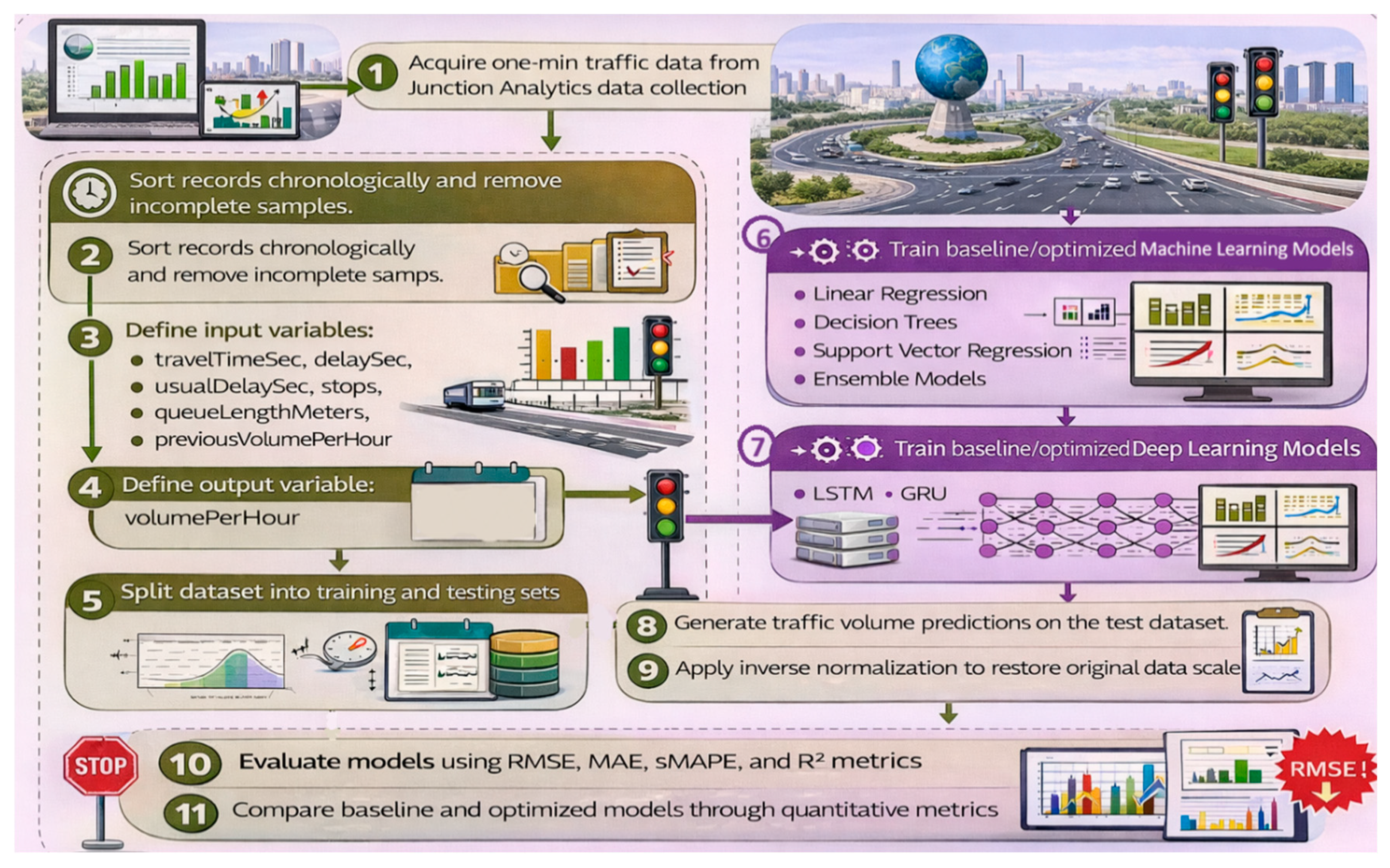
As illustrated in Figure 1, the proposed traffic load prediction framework adopted in this study consists of a structured sequence of data preparation, model development, prediction, and evaluation stages. All of these steps are designed to ensure a fair and consistent comparison between the proposed ML- and DL-based traffic load prediction models.

First, one-minute traffic data are acquired from the TomTom Junction Analytics system (Step 1). The dataset contains multiple traffic-related variables collected at a major urban roundabout in Jeddah. To preserve temporal integrity, incomplete or corrupted samples are removed and the remaining records are arranged chronologically (Step 2).

Next, the input variables used for prediction are defined (Step 3). These variables include travel time (travelTimeSec), delay (delaySec), usual delay (usualDelaySec), number of stops (stops), queue length (queueLengthMeters), and historical traffic volume (previousVolumePerHour). The target output variable is defined as the current traffic volume per hour (volumePerHour), which represents the primary response variable of the prediction task (Step 4).

The dataset is then partitioned into training and testing subsets to ensure that test observations are not used during model development, thereby maintaining the reliability of the evaluation process (Step 5). As part of the preprocessing stage, the input variables are normalized using statistics derived exclusively from the training data to ensure consistent scaling and numerical stability.

Following data preprocessing, baseline and optimized machine learning (ML) models are trained (Step 6). These models include linear regression, decision tree–based models, support vector regression, and ensemble learning techniques. In parallel, baseline and optimized deep learning (DL) models, including LSTM and GRU architectures, are developed to capture temporal dependencies inherent in traffic data (Step 7).

After model training, traffic volume predictions are generated for the test dataset (Step 8). The predicted values are then transformed back to their original scale using inverse normalization to enable direct comparison with the observed traffic volumes (Step 9). The predictive performance of each model is evaluated using several statistical error metrics (Step 10). Finally, baseline and optimized models across both ML and DL configurations are compared using quantitative metrics and visual analyses to assess prediction accuracy and robustness (Step 11).

After presenting the overall traffic load prediction framework illustrated in Figure 1, the following subsections describe the methodological components of the proposed study in detail. First, the traffic dataset and preprocessing procedures are introduced, including data cleaning, feature definition, normalization, and dataset partitioning. Next, the predictive modeling approaches are presented, covering both baseline and optimized configurations of machine learning and deep learning models. Subsequently, the evaluation metrics used to assess prediction accuracy are defined. Finally, the comparative evaluation framework is described to ensure a fair and consistent assessment of all predictive models.

2.1. Data Description and Preprocessing

The proposed study utilizes real-time traffic data obtained from the Earth Globe Roundabout in Jeddah, Saudi Arabia. This major urban intersection experiences heavy traffic demand. The real-time traffic data has been collected using TomTom Junction Analytics platform and comprise one-minute resolution measurements gathered during the month of March. It should be noted that TomTom Junction Analytics provides probe-based traffic estimates derived from floating vehicle data rather than direct sensor measurements. Consequently, the dataset may contain estimation uncertainty inherent to probe-based traffic analytics. However, the use of high-resolution, probe-based traffic data guarantees that the ensuing modeling process is anchored in real-world traffic conditions and facilitates dependable data-driven forecasting.

Prior to model development, the dataset was carefully examined to identify missing values, inconsistencies, and temporal misalignments. All traffic variables were synchronized to a common one-minute time scale to ensure temporal consistency across the observations. Records containing incomplete or corrupted entries were removed during the preprocessing stage.

The final dataset covers the entire month of March 2025, spanning from 1 March 2025 (00:00) to 31 March 2025 (23:59), and contains 44,622 one-minute observations collected at the Earth Globe Roundabout in Jeddah, Saudi Arabia. The dataset includes both weekdays (Sunday–Thursday) and weekends (Friday–Saturday), providing a comprehensive representation of typical urban traffic conditions. The observation period partially overlaps with the Ramadan season in Saudi Arabia, which may influence travel demand patterns due to changes in daily activity schedules. No days were removed due to missing data or sensor failures, ensuring continuous temporal coverage throughout the study period.

The study utilizes a data-driven framework to facilitate a consistent and fair comparative evaluation of the selected prediction models, defining input and output variables based on measurable traffic conditions commonly found in modern Intelligent Transportation Systems (ITS). There are two main reasons for choosing the variables: (i) to accurately show the important operational characteristics of urban traffic flow at intersections, and (ii) to make sure that the chosen features are useful for predicting short-term traffic volume in real-world situations. The proposed formulation employs traffic indicators that reflect both current conditions and short-term temporal context, allowing the models to effectively encapsulate congestion dynamics, traffic unpredictability, and short-term dependencies in a realistic and operationally relevant manner. As shown below, the traffic dataset is organized by listing a set of explanatory input variables and one target output variable.

The selected input variables are:

• travelTimeSec: Travel time through the junction approach (seconds);
• delaySec: Observed traffic delay relative to free-flow conditions (seconds);
• usualDelaySec: Typical delay expected for the same time of day and day of week (seconds);
• stops: Average number of stops per vehicle;
• queueLengthMeters: Estimated queue length on the approach (meters);
• previousVolumePerHour: Traffic volume observed in the previous time step (vehicles/hour).

The selected output variable is:

• volumePerHour: Traffic volume passing through the junction approach (vehicles/hour).

For improved readability, the variable names shown in tables are presented in simplified descriptive form (e.g., Travel Time (s) instead of travelTimeSec), while maintaining the same definitions and measurement units as the original dataset variables.

Table 1. Sample of collected traffic dataset for The Earth Globe Roundabout (Jeddah) during March (one-minute resolution).

Date	Time	Travel Time (s)	Delay (s)	Usual Delay (s)	Stops	Queue Length (m)	Traffic Volume (veh/h)
01-03-2025	1:40:02	54	35	12	0.51	76.15	941
01-03-2025	1:41:01	48	29	13	0.49	88.02	880
01-03-2025	1:42:01	44	25	13	0.53	79.55	819
01-03-2025	1:43:01	43	24	13	0.55	67.81	844
01-03-2025	1:44:02	59	40	14	0.50	63.12	813
01-03-2025	1:45:01	60	41	14	0.49	82.81	808
01-03-2025	1:46:02	41	22	14	0.51	62.51	805
01-03-2025	1:47:01	37	18	15	0.50	54.40	787
01-03-2025	1:48:02	24	5	15	0.42	79.33	801
01-03-2025	1:49:02	12	0	15	0.43	64.12	743

presents a representative sample of the traffic dataset collected at the Earth Globe Roundabout in Jeddah during March 2025. Each record captures the instantaneous traffic state at the junction, combining temporal information (date and time) with multiple operational traffic indicators. The variables reflect key aspects of traffic performance, including travel time, observed and usual delays, stopping behavior, queue formation, and traffic volume. As illustrated in the table, noticeable variations occur over consecutive minutes, even within a short time window, highlighting the highly dynamic nature of urban traffic flow. For instance, fluctuations in travel time and delay are accompanied by changes in queue length and traffic volume, indicating the interaction between congestion buildup and discharge processes at the junction. This fine-grained temporal variability underscores the need for predictive models capable of capturing rapid short-term changes and complex temporal dependencies.

Specifically, the sample records show that periods with higher travel time and delay values (e.g., at 01:44–01:46) are associated with longer queues and elevated traffic volumes, whereas lower travel time and delay values (e.g., at 01:47–01:48) coincide with reduced queue lengths and a noticeable decline in traffic volume. This relationship illustrates how congestion intensity and queue dynamics directly influence short-term traffic load, confirming the suitability of the dataset for short-term traffic volume prediction under real operational conditions.

To better characterize the dataset used for model development, descriptive statistics were computed for all traffic variables involved in the prediction framework.

Table 2. Descriptive statistics of the traffic variables used in the prediction models.

Variable	Mean	Std	Min	Median	Max
Travel Time (s)	47.54	33.91	7	37	362
Delay (s)	29.81	33.36	0	19	344
Usual Delay (s)	24.89	9.49	0	25	52
Stops	0.51	0.24	0	0.44	1.79
Queue Length (m)	382.44	383.74	0	204.27	4879.7
Traffic Volume (veh/h)	2325.94	1493.17	0	2058	8933

presents the main statistical indicators, including the mean, standard deviation, minimum, median, and maximum values. These statistics provide an overview of the variability and distribution of traffic conditions at the Earth Globe Roundabout during the observation period.

The results indicate substantial variability in traffic conditions at the Earth Globe Roundabout. The average traffic volume is approximately 2326 vehicles per hour, with peak values approaching 9000 vehicles per hour during high-demand periods. Similarly, the average vehicle delay is approximately 30 s, while extreme congestion conditions may increase delays to more than 300 s. These variations highlight the dynamic and nonlinear nature of traffic conditions at the study location, which motivates the application of advanced machine learning and deep learning models for short-term traffic prediction.

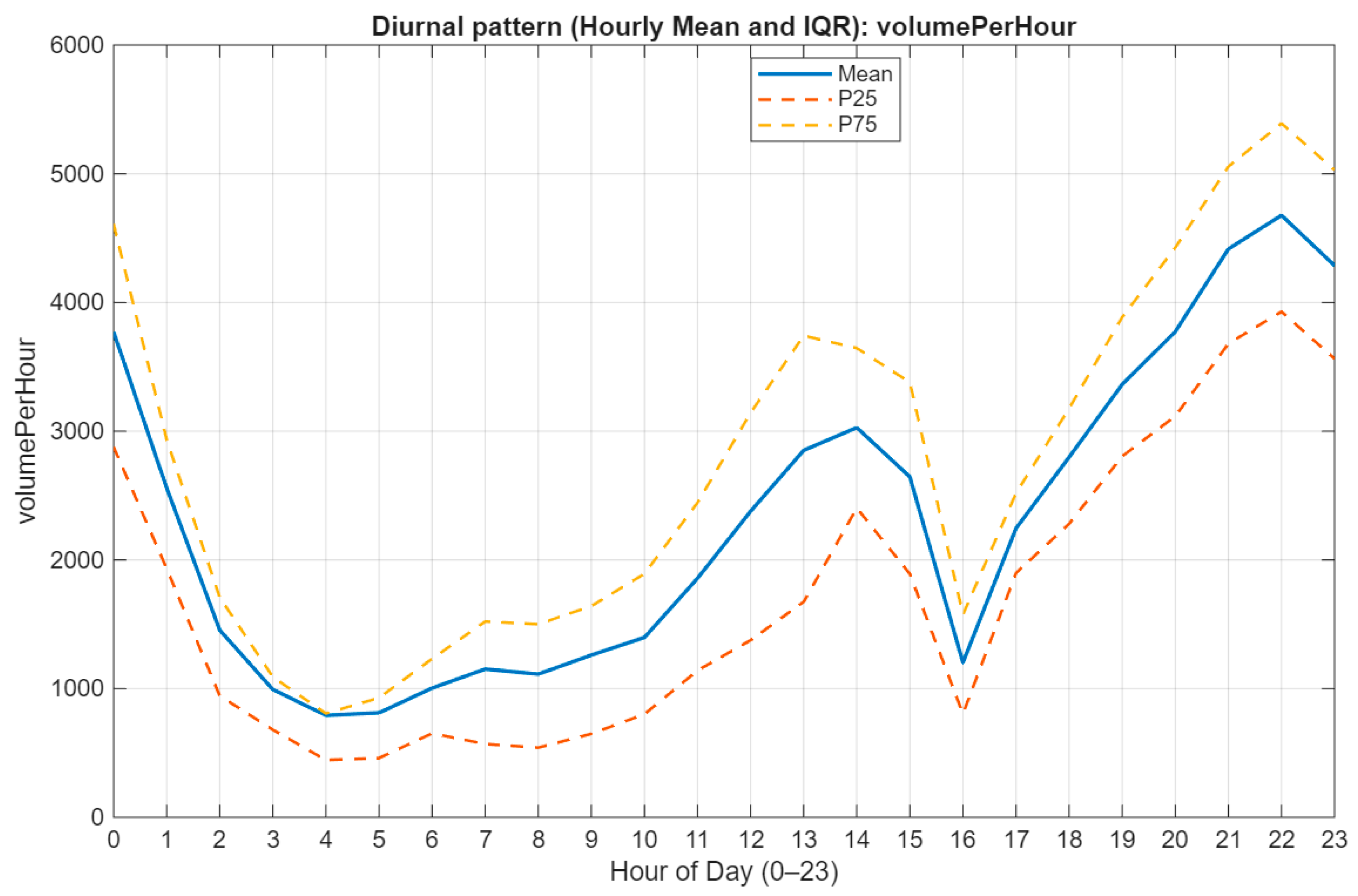
To further illustrate the temporal characteristics of the traffic conditions, Figure 2 and Figure 3 present the diurnal patterns of traffic volume and vehicle delay aggregated by hour of day. Figure 2 shows that traffic demand follows a clear daily cycle, with lower traffic volumes during nighttime hours and pronounced increases during daytime and evening periods. The peak traffic volumes occur during the late afternoon and evening hours, reflecting typical urban commuting patterns.

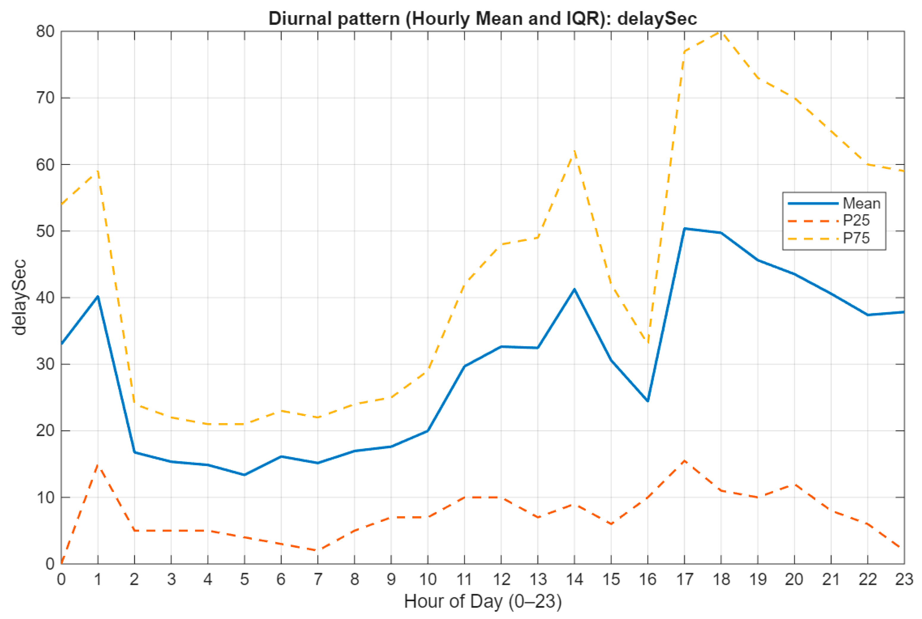
Figure 3 presents the corresponding hourly delay pattern, which closely follows the variations in traffic demand. Delay values remain relatively low during off-peak hours but increase significantly during periods of higher traffic volume. The interquartile ranges shown in both figures highlight the variability of traffic conditions throughout the day, indicating that the traffic system experiences both stable low-demand periods and highly variable peak periods. These temporal dynamics demonstrate the complexity and nonlinearity of traffic behavior at the studied roundabout, reinforcing the need for advanced prediction models capable of capturing short-term traffic fluctuations.

These observed temporal patterns confirm the presence of strong daily traffic regimes, which further motivates the need for predictive models capable of capturing both short-term fluctuations and recurring traffic cycles.

To enhance numerical stability, accelerate model convergence, and ensure balanced feature contribution across variables with different physical scales, z-score normalization was applied to all input variables. Each input feature $x$ was normalized according to:

$$x_{\mathrm{norm}}={\displaystyle \frac{x-\mu }{\sigma }}$$

(1)

where $\mu$ and $\sigma$ denote the mean and standard deviation of the corresponding feature, respectively. Importantly, these statistics were computed exclusively from the training dataset and subsequently applied to the testing dataset to prevent information leakage and preserve the integrity of the evaluation process. This normalization strategy is particularly important for learning algorithms, as it prevents features with larger numerical ranges from dominating the training process and improves the stability of optimization across different model types.

Following model inference, all predicted traffic volumes were transformed back to their original scale prior to performance evaluation. This ensured that error metrics were computed in physically interpretable units (vehicles/hour), facilitating meaningful comparison across models.

To preserve temporal dependencies and reflect realistic deployment conditions, the dataset was partitioned chronologically rather than using random sampling. First, 80% of the observations were used as the development set, while the remaining 20% were strictly held out as an independent test set for final performance evaluation. Within the development set, the last 10% of the timeline was reserved as a validation subset, while the remaining 90% was used for model training. Consequently, the effective dataset split corresponds approximately to 72% training, 8% validation, and 20% testing, all defined chronologically.

This design ensures that the test data represent unseen future observations and are not used during model development, thereby providing a realistic evaluation of model performance for future traffic prediction.

To prevent information leakage during model development, all hyperparameter optimization procedures were restricted to the training data. For the machine learning (ML) models implemented in the MATLAB R2025b Regression Learner App, Bayesian hyperparameter optimization was conducted using internal k-fold cross-validation within the training subset only. For deep learning models (LSTM and GRU), the training portion was chronologically divided into a training block and a validation block, where the validation block corresponds to the last segment of the development set. Bayesian optimization minimized the validation RMSE on normalized targets, and after the optimal hyperparameters were identified, the final model was retrained on the full training subset and evaluated once on the untouched test set.

To enable short-term temporal learning for the recurrent deep learning models, the multivariate traffic time series was converted into a sliding-window sequence representation with a window length of 10 min (i.e., 10 consecutive one-minute observations). Each input sample therefore consists of a 10-step temporal sequence of the six explanatory variables, representing the traffic conditions during the previous 10 min, while the target output corresponds to the traffic volume at the next prediction step. This sequence formulation allows the recurrent networks to capture short-term temporal dependencies and dynamic traffic fluctuations. The windowing procedure was applied consistently to both baseline and optimized deep learning models while maintaining the chronological data split and strict isolation of the test dataset.

2.2. Prediction Models

Based on the data preparation, normalization, and chronological partitioning described in the previous section, short-term traffic load prediction is formulated as a supervised learning problem. This study evaluates a set of regression-based machine learning (ML) and deep learning (DL) models within a systematic comparative framework. All models are trained and tested using the same input–output formulation, normalized feature space, and training–testing split to ensure a fair and consistent performance comparison.

The modeling process encompasses three main stages: model development, prediction, and performance evaluation. Both baseline and optimized model configurations are considered to assess robustness under varying traffic conditions. Where applicable, hyperparameter tuning is conducted using Bayesian optimization with an expected improvement acquisition function, providing an efficient and objective parameter selection process without manual intervention. For regression-based models, Bayesian optimization was conducted using internal 5-fold cross-validation within the training set. For deep learning models, all hyperparameter tuning and model development procedures were restricted to the training subset. The test set was strictly reserved for final performance evaluation to avoid information leakage.

2.2.1. Regression-Based Machine Learning Models

Regression-based ML models were developed to provide baseline and advanced predictive benchmarks for short-term traffic load forecasting. For each approach, a baseline configuration was first implemented, followed by an optimized version in which key hyperparameters were tuned to enhance predictive accuracy and generalization capability. All models utilized the same six input features—travel time, delay, usual delay, number of stops, queue length, and previous traffic volume—without applying dimensionality reduction in order to preserve the physical interpretability of traffic features and ensure a fair comparison across models.

Linear Regression (LR) was employed as a baseline model to capture linear relationships between traffic-related variables and hourly traffic volume. The model was formulated using ordinary least squares estimation and trained using all six input features without regularization or feature transformation. As LR does not involve tunable hyperparameters in the present formulation, no optimized variant was considered. This model serves as a reference for evaluating the performance gains achieved by nonlinear methods.

Regression tree models were used to capture nonlinear decision structures in traffic data. The baseline median tee configuration, referred to as Med Tree, employed a single regression tree with a minimum leaf size of 12, with surrogate decision splits disabled to control model complexity.

The optimized regression tree model, referred to as OptTree, was developed by tuning the minimum leaf size parameter using Bayesian optimization. The optimization process explored a wide search range and selected a minimum leaf size of 50, which improved model generalization by reducing overfitting while preserving interpretability.

Support Vector Machine (SVM) models were applied to represent nonlinear traffic patterns using a kernel-based learning framework. The baseline SVM employed a Gaussian kernel with a kernel scale of 0.61, while the box constraint and epsilon parameters were automatically selected. Input data standardization was not applied.

The optimized SVM variant (OptSVM) was obtained through Bayesian hyperparameter optimization. The optimization process selected a quadratic kernel function, a box constraint of 0.0034, and an epsilon value of 0.0571. These adjustments enabled the optimized SVM to achieve improved predictive accuracy and robustness compared to the baseline configuration.

Ensemble learning models were developed to enhance robustness by aggregating multiple regression trees. The baseline Ensemble model employed a bagging strategy consisting of 30 regression trees, each with a minimum leaf size of 8. Predictions were obtained by averaging the outputs of individual learners.

The optimized ensemble model (OptEnsemble) adopted a boosting-based strategy using Least Squares Boosting (LSBoost). Bayesian optimization was applied to tune key hyperparameters, including the number of learners, learning rate, minimum leaf size, and the number of predictors sampled at each split. The optimized configuration consisted of 174 learners, a learning rate of 0.2798, and a minimum leaf size of 1, resulting in enhanced predictive performance.

Feedforward neural networks were employed as nonlinear regression models. The baseline neural network (NN) consisted of a single hidden layer with 25 neurons and a sigmoid activation function. The model was trained for 50 iterations without regularization, providing a nonlinear baseline with moderate complexity.

The optimized neural network model (OptNN) was developed by tuning network depth, neuron counts, activation functions, and regularization strength. The optimized configuration consisted of three fully connected hidden layers with neuron sizes of 29, 1, and 1, respectively, and a regularization parameter of $\lambda =4.29\times {10}^{-7}$. Bayesian optimization was employed to identify optimal architecture and parameter values. This configuration was selected automatically by Bayesian optimization, indicating that a simpler architecture was sufficient for capturing the dominant patterns in the dataset.

2.2.2. Deep Learning Models

To capture temporal dependencies and sequential traffic patterns inherent in high-resolution traffic data, deep learning (DL) models based on Long Short-Term Memory (LSTM) and Gated Recurrent Unit (GRU) architectures were developed. Both architectures were evaluated under baseline and optimized configurations to examine the impact of hyperparameter tuning on predictive performance. All deep learning models processed multivariate traffic sequences using a sequence-to-one learning strategy, enabling effective modeling of short-term dynamics and temporal correlations in the observed traffic conditions.

The proposed deep learning framework receives a short historical window of multivariate traffic observations and predicts the traffic volume at the next time step. In the present study, the input sequence length was set to 10 time steps (corresponding to 10 min of historical data), while the prediction horizon was one minute ahead. Each input sequence contains six explanatory variables representing the traffic state, namely travel time, delay, usual delay, stops, queue length, and the previous traffic volume.

For both LSTM and GRU architectures, the baseline configuration consists of a single recurrent layer followed by a fully connected layer and a regression output layer. The baseline models use 32 hidden units, a mini-batch size of 128, and are trained for 50 epochs using the Adam optimizer with an initial learning rate of 0.01. To improve numerical stability during training, gradient clipping with a threshold value of 1 was applied. The chronological order of the time-series data was preserved during training by disabling data shuffling.

Hyperparameter tuning was conducted using Bayesian optimization to systematically explore the configuration space of the deep learning models. The optimization process considered four key hyperparameters: the number of hidden units (10–60), the maximum number of training epochs (10–60), the initial learning rate (10⁻²–10⁻¹), and the learning rate drop factor (10⁻²–0.5). Logarithmic scaling was applied to the learning rate and drop factor to enable efficient exploration across several orders of magnitude.

The objective function minimized the validation mean squared error (MSE) computed on a temporally separated validation subset extracted from the training data. A maximum set of 50 Bayesian optimization iterations was performed using the expected-improvement acquisition function. This procedure ensured that model tuning was conducted exclusively on the training data, preventing information leakage from the test set and enabling a fair comparison of model performance. The final hyperparameter configurations selected by the Bayesian optimization procedure are summarized in

Table 3. Optimal hyperparameter configurations identified by Bayesian optimization for the deep learning models used in the traffic load prediction framework.

Model	Hidden Units	Max Epochs	Initial Learning Rate	Learning Rate Drop Factor
OptLSTM	54	13	0.024567	0.20802
OptGRU	52	47	0.010397	0.058149

.

The optimized LSTM model employed 54 hidden units and was trained for 13 epochs with an initial learning rate of 0.024567 and a learning rate drop factor of 0.20802. The optimized GRU model used 52 hidden units and 47 training epochs, with an initial learning rate of 0.010397 and a drop factor of 0.058149. These configurations correspond to the best-performing solutions identified during the 50 optimization iterations based on the minimum validation error.

2.3. Model Evaluation Metrics

Model performance was evaluated by using multiple statistical error metrics to provide a comprehensive assessment of prediction accuracy and robustness. The selected metrics quantify different aspects of performance, including error magnitude, sensitivity to scale, and goodness of fit. All metrics were computed on the test dataset after applying inverse normalization to restore predicted traffic volumes to their original physical scale (vehicles/hour), ensuring an interpretable and consistent comparison across models.

The evaluation metrics used in this study are defined as follows:

Mean Squared Error (MSE):

$$\mathrm{MSE}={\displaystyle \frac{1}{N}}{\sum }_{i=1}^N{(y_i-{\widehat{y}}_i)}^2$$

(2)

where $y_i$ represents the actual traffic volume, ${\widehat{y}}_i$ denotes the predicted traffic volume, and $N$ is the total number of test samples.

Root Mean Squared Error (RMSE):

$$\mathrm{RMSE}=\sqrt{{\displaystyle \frac{1}{N}}{\sum }_{i=1}^N(y_i-{\widehat{y}}_i{)}^2}$$

(3)

RMSE penalizes large errors more heavily and is widely used in traffic forecasting due to its sensitivity to significant deviations.

Mean Absolute Error (MAE):

$$\mathrm{MAE}={\displaystyle \frac{1}{N}}{\sum }_{i=1}^N\mid y_i-{\widehat{y}}_i\mid$$

(4)

MAE provides a direct measure of average prediction error magnitude and is less sensitive to outliers than RMSE.

Symmetric Mean Absolute Percentage Error (sMAPE):

$$\mathrm{sMAPE}={\displaystyle \frac{100}{N}}{\sum }_{i=1}^N{\displaystyle \frac{\mid y_i-{\widehat{y}}_i\mid }{\left(\mid y_i\mid +\mid {\widehat{y}}_i\mid \right)/2}}$$

(5)

sMAPE expresses prediction accuracy as a percentage using a symmetric formulation that reduces the bias of traditional MAPE, particularly when actual values are close to zero. In cases where both actual and predicted values approach zero, a small numerical constant was added to the denominator to prevent division-by-zero errors.

Coefficient of Determination (R²):

$$R^2=1-{\displaystyle \frac{{\sum }_{i=1}^N(y_i-{\widehat{y}}_i{)}^2}{\sum _{i=1}^N(y_i-\overline{y}{)}^2}}$$

(6)

where $\overline{y}$ denotes the mean of the observed traffic volumes. $R^2$ measures the proportion of variance in the observed data explained by the model.

2.4. Comparative Evaluation Framework

To ensure a fair and consistent comparison, all models were trained and tested using identical dataset partitions, input variables, and evaluation procedures. Results were analyzed by comparing:

• Baseline versus optimized model configurations, to quantify the impact of systematic hyperparameter tuning on prediction accuracy, temporal stability, and error behavior;
• Regression-based ML models versus DL models, to assess differences in their ability to capture nonlinear relationships and temporal dependencies in high-resolution traffic data;
• Temporal prediction behavior under different traffic conditions, examined through full-range and zoomed-in visual analyses, with particular focus on peak periods, rapid traffic transitions, and congestion recovery phases.

This structured evaluation framework allows clear identification of the most effective prediction models while maintaining practical relevance for real-world traffic management applications.

2.5. Variability-Based Regime Definition

To examine whether model performance changes under different traffic demand dynamics, we conducted a variability-based regime analysis on the test set. A variability score was computed as the rolling standard deviation of the target traffic load using a 30-min sliding window. Based on percentile thresholds of this score, test samples were categorized into high-variability (top 30%) and low-variability (bottom 30%) regimes. Performance metrics were then computed separately for each regime to evaluate context-dependent behavior.

All experiments were conducted using MATLAB R2025b. Regression-based models were developed using the Regression Learner App, while deep learning models were implemented through MATLAB scripting. This unified environment supports reproducibility and enables consistent implementation of both ML and DL models within a single analytical pipeline.

3. Results and Discussion

This section presents a comprehensive comparative evaluation of baseline and optimized machine learning (ML) and deep learning (DL) models for short-term traffic load prediction using real-world data collected from major urban corridors in Saudi Arabia. The analysis combines global performance indicators with detailed assessment of temporal prediction behavior, enabling an in-depth evaluation of prediction accuracy, robustness, and practical applicability for intelligent transportation systems.

3.1. Overall Prediction Performance

Table 4. Performance comparison of all the proposed prediction models.

ModelName	Type	MSE	RMSE	MAE	sMAPE	R2
GRU	Baseline	49,012	221.387	164.970	9.479	0.974
OptGRU	Optimized	22,237	149.122	108.179	5.787	0.988
LSTM	Baseline	31,898	178.601	127.314	6.683	0.983
OptLSTM	Optimized	22,757	150.854	108.285	5.500	0.988
SVM	Baseline	226,290	475.698	241.539	10.641	0.880
OptSVM	Optimized	28,297	168.216	113.624	5.335	0.985
MedTree	Baseline	36,013	189.772	129.330	6.028	0.981
OptTree	Optimized	30,004	173.218	118.050	5.586	0.984
Ensemble	Baseline	30,010	173.233	117.766	5.543	0.984
Opt Ensemble	Optimized	30,448	174.495	117.194	5.459	0.984
NN	Baseline	29,773	172.548	117.779	5.752	0.984
OptNN	Optimized	29,681	172.283	116.474	5.700	0.984
LR	Baseline	29,681	172.282	116.474	5.700	0.984

presents the quantitative performance comparison between baseline and optimized machine learning (ML) and deep learning (DL) models for traffic volume prediction at the Earth Globe Roundabout in Jeddah. Model performance is evaluated using multiple error metrics, including MSE, RMSE, MAE, sMAPE, and R², providing a comprehensive assessment of prediction accuracy and goodness of fit.

The results in Table 4 indicate that the optimized deep learning models achieve the highest prediction accuracy among all evaluated approaches. In particular, the optimized GRU (OptGRU) achieves the lowest RMSE of 149.12 veh/h, closely followed by the optimized LSTM (OptLSTM) with an RMSE of 150.85 veh/h. Both optimized recurrent models also obtain the highest coefficient of determination (R² ≈ 0.988), indicating a strong ability to capture the temporal patterns of traffic demand.

Among the machine learning models, OptSVM provides the best performance with an RMSE of 168.22 veh/h, representing a substantial improvement compared to the baseline SVM (RMSE = 475.70 veh/h). This result highlights the importance of hyperparameter optimization when applying kernel-based models to complex urban traffic data.

Several baseline models such as LR, NN, and Ensemble show relatively similar performance levels, with RMSE values around 172–173 veh/h and R² ≈ 0.984, indicating that short-term traffic patterns at the studied roundabout exhibit partially predictable and quasi-linear behavior. The nearly identical performance of LR and OptNN suggests that the optimized neural network effectively approximated a near-linear mapping.

In contrast, the baseline recurrent models (GRU and LSTM) show weaker performance compared to their optimized counterparts, confirming that deep learning architectures are highly sensitive to training configuration and benefit significantly from hyperparameter optimization.

Overall, the performance ranking can be summarized as follows:

Optimized DL models (OptGRU ≈ OptLSTM) > Optimized ML models > Baseline ML models > Baseline DL models.

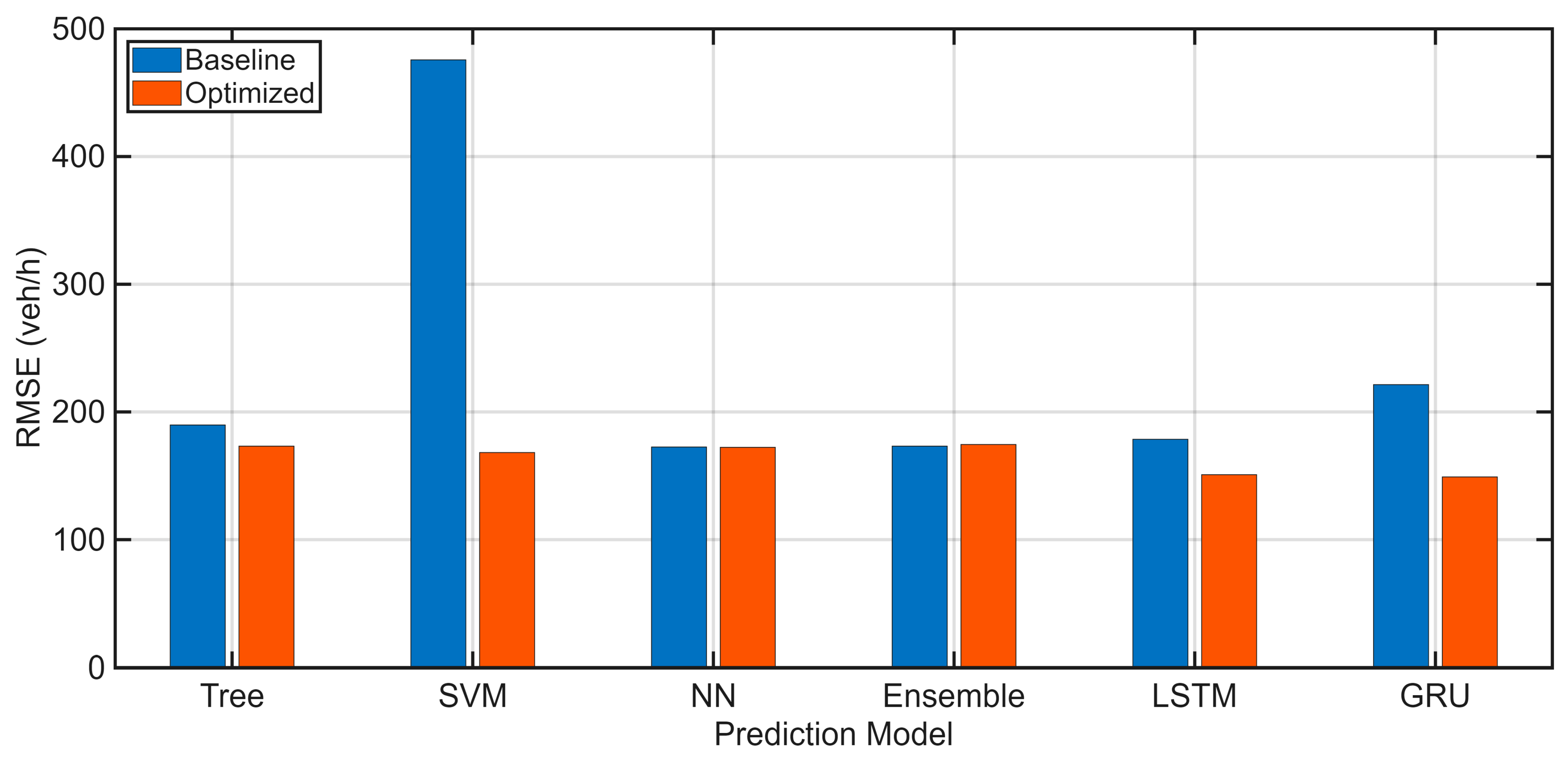
Figure 4 illustrates the comparison of Root Mean Square Error (RMSE) values between baseline and optimized prediction models across different ML and DL approaches. The results clearly demonstrate that hyperparameter optimization leads to substantial performance improvements across all evaluated model families.

Among the baseline models, linear regression (LR), neural networks (NN), and ensemble learning exhibit relatively competitive performance, achieving RMSE values of approximately 172–173 veh/h. In contrast, baseline support vector machines (SVM) and deep learning models show noticeably higher error levels. In particular, the baseline SVM exhibits the highest RMSE, exceeding 475 veh/h, while the baseline GRU and LSTM models show RMSE values of 221.39 veh/h and 178.60 veh/h, respectively. This behavior highlights the sensitivity of complex nonlinear and recurrent models to hyperparameter selection and training configuration when applied without systematic tuning.

Following optimization, a clear reduction in prediction error is observed across most models. The optimized GRU (OptGRU) achieves the lowest RMSE of 149.12 veh/h, closely followed by the optimized LSTM (OptLSTM) with an RMSE of 150.85 veh/h, outperforming all regression-based machine learning approaches. Optimized SVM, tree-based, and neural network models also demonstrate substantial improvements relative to their baseline counterparts, confirming the effectiveness of Bayesian hyperparameter optimization in enhancing predictive accuracy.

The relatively strong baseline performance of the linear regression model can be attributed to the structured traffic patterns typically observed at major urban roundabouts in Saudi Arabia, where regulated traffic flow and consistent daily demand patterns often produce partially linear relationships between traffic variables and traffic volume. These conditions allow simple models to capture overall trends effectively. Nevertheless, linear regression remains limited in representing nonlinear dynamics and sudden traffic fluctuations, which are better captured by optimized deep learning architectures.

Overall, the results presented in Figure 4 highlight the importance of systematic model tuning and demonstrate the superior predictive capability of optimized recurrent deep learning models for short-term traffic load prediction.

However, aggregate performance metrics may mask regime-dependent behavior under fluctuating traffic conditions. Therefore, a variability-based regime analysis is conducted in the following subsection to examine contextual performance differences.

3.2. Variability-Based Regime Analysis

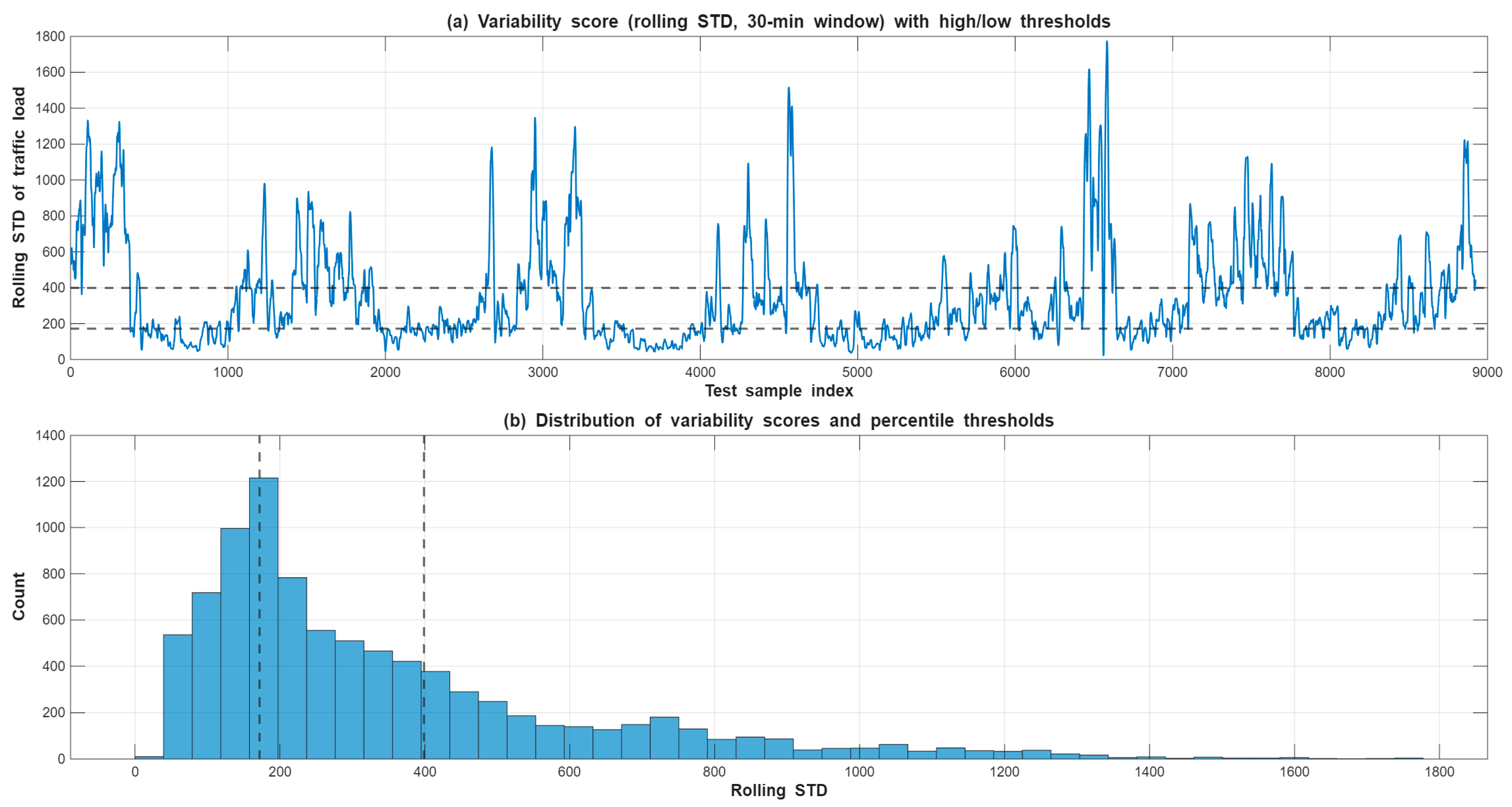
To further investigate whether model performance remains consistent under different traffic demand dynamics, a variability-based regime analysis was conducted on the test dataset. A rolling standard deviation (30-min window) of the target traffic volume was used to quantify short-term demand fluctuations. Based on percentile thresholds, test samples were categorized into high-variability (top 30%) and low-variability (bottom 30%) regimes. Figure 5 illustrates the variability score and the selected thresholds.

As shown in Figure 5a, the variability score exhibits clear temporal fluctuations with intermittent high-intensity bursts and relatively stable periods. The percentile-based thresholds define the boundaries between high- and low-variability regimes. The distribution presented in Figure 5b further illustrates the heterogeneous nature of the traffic dynamics, characterized by a right-skewed distribution of variability scores. This observation supports evaluating model performance separately under different demand regimes.

Based on this regime definition, model performance was evaluated separately under high- and low-variability conditions.

As reported in

Table 5. Model performance under variability-based regimes.

Model	MAE (Overall)	RMSE (Overall)	MAE (HighVar)	RMSE (HighVar)	MAE (LowVar)	RMSE (LowVar)	p-Value vs. Best
GRU	164.970	221.387	232.083	296.316	107.090	131.721	0
OptGRU	108.179	149.122	162.156	206.828	62.301	79.714	1
LSTM	127.314	178.601	192.513	248.434	69.461	91.421	3.36 × 10−44
OptLSTM	108.285	150.854	160.423	205.816	60.976	81.677	0.2871
SVM	241.539	475.698	434.373	730.816	129.808	298.504	0
OptSVM	113.624	168.216	191.425	251.472	50.813	69.527	0.5358
MedTree	129.330	189.772	211.652	276.943	58.034	80.220	2.34 × 10−29
OptTree	118.050	173.218	198.562	255.860	50.246	70.115	0.0023
Ensemble	117.766	173.233	196.940	255.774	51.424	71.064	0.0201
Opt Ensemble	117.194	174.495	198.980	261.541	50.581	69.326	0.2067
NN	117.779	172.548	195.817	256.153	55.619	75.171	0.0002
OptNN	116.474	172.283	196.997	258.604	51.837	71.075	0.0632
LR	116.474	172.282	196.997	258.603	51.837	71.075	0.0632

, the optimized GRU model achieves the best overall predictive performance with the lowest RMSE (149.12 veh/h) and MAE (108.18 veh/h). The optimized LSTM model shows comparable performance (RMSE = 150.85 veh/h), indicating that both optimized recurrent architectures effectively capture the short-term temporal dynamics of traffic demand.

Under high-variability conditions, the optimized GRU and optimized LSTM models remain the most robust, achieving RMSE values of 206.83 veh/h and 205.82 veh/h, respectively. In contrast, several conventional machine learning models exhibit noticeably higher errors in these highly dynamic periods. This behavior reflects the stronger capability of recurrent neural networks to model nonlinear temporal dependencies during rapidly changing traffic states.

Under low-variability conditions, however, several optimized machine learning models become highly competitive. In particular, optimized tree-based and SVM models achieve the lowest MAE values (≈50–51 veh/h), slightly outperforming deep learning models in stable traffic regimes where temporal dynamics are less complex.

To assess statistical significance, the Wilcoxon signed-rank test was applied to paired absolute prediction errors relative to the best overall model (OptGRU). The results indicate that many baseline models show statistically significant differences (p < 0.01), whereas several optimized machine learning models (e.g., OptSVM and OptEnsemble) do not exhibit statistically significant differences compared with the best model. This confirms that performance differences among the top models are relatively small under certain operating conditions.

Overall, the regime-based analysis highlights that model effectiveness depends strongly on traffic demand variability. Optimized recurrent neural networks provide greater robustness under highly dynamic traffic conditions, while optimized classical machine learning models remain competitive in stable regimes. These findings emphasize that relying solely on aggregate performance metrics may obscure meaningful differences in model behavior across operational traffic states. The results also demonstrate that Bayesian hyperparameter optimization substantially improves the performance of recurrent models compared with their baseline counterparts.

3.3. Baseline Models: Temporal Behavior and Limitations

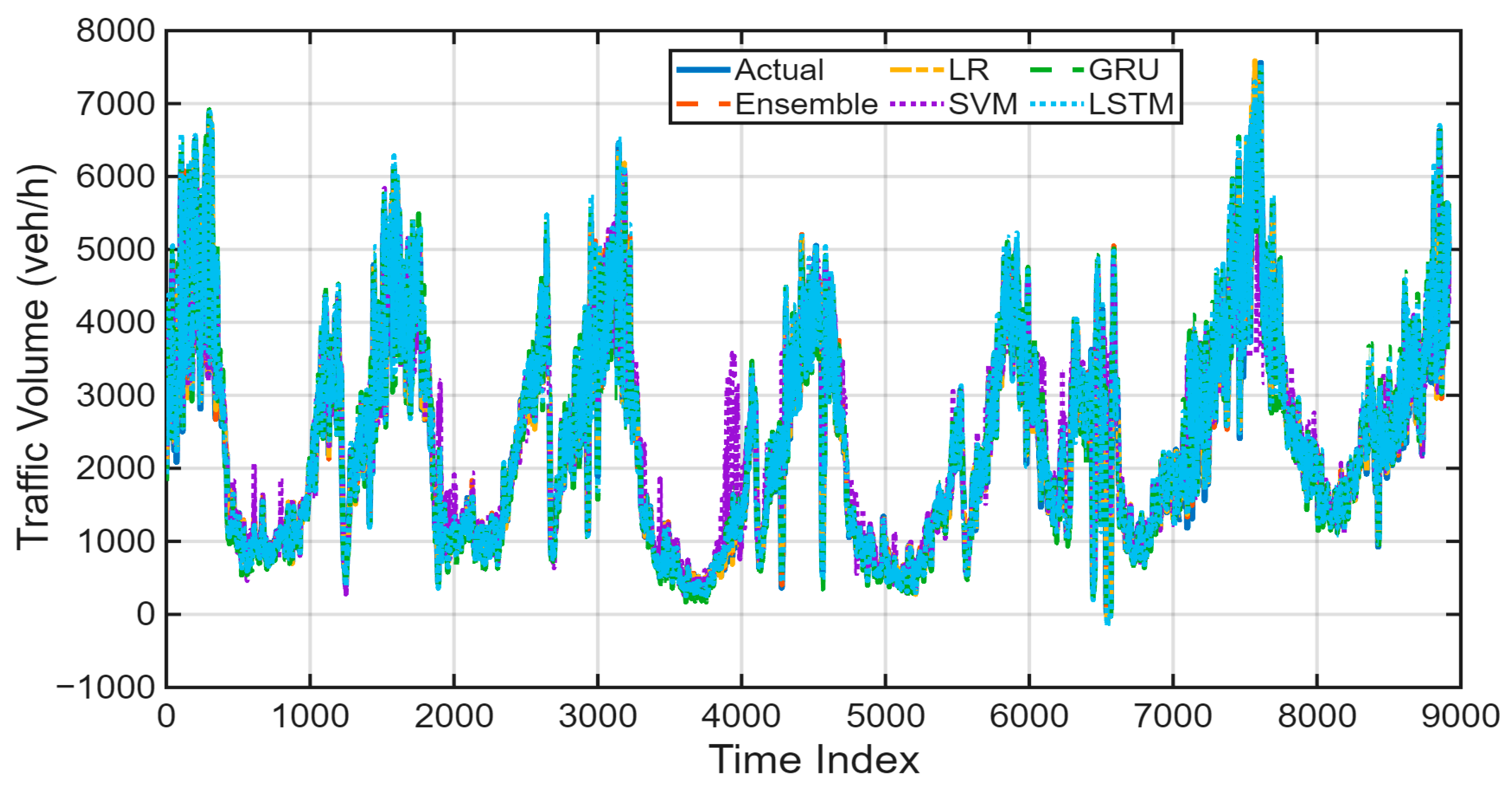
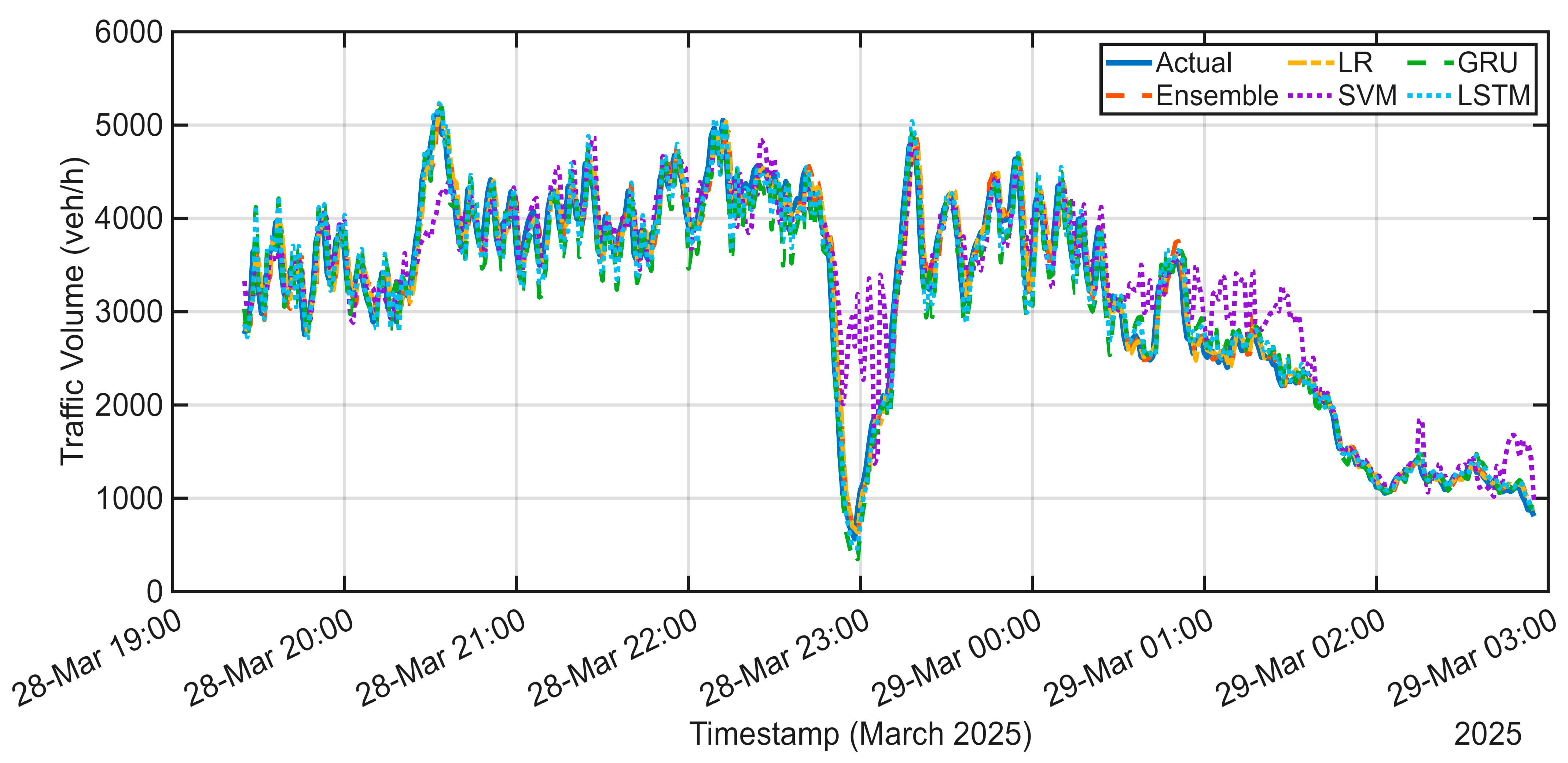
Figure 6 and Figure 7 present the full-range and zoomed-in temporal comparisons between the actual traffic volumes and the predictions generated by the baseline models.

The full-range results shown in Figure 6 indicate that baseline models are generally capable of capturing the overall diurnal traffic patterns, including morning and evening peak periods as well as off-peak intervals. This indicates that the models are able to learn the dominant periodic structure of traffic demand observed at the studied roundabout.

Despite this general agreement with the observed traffic patterns, noticeable deviations emerge during periods of rapid traffic variation and sudden congestion transitions. In particular, several baseline models tend to smooth sharp changes in traffic volume, leading to slight underestimation of peak traffic levels and mild overestimation during abrupt drops. These discrepancies become more evident during highly dynamic traffic conditions, where short-term fluctuations dominate traffic flow behavior.

The zoomed-in analysis presented in Figure 7 provides additional insight into short-term prediction behavior. Linear regression and ensemble models produce relatively smooth approximations that follow the overall trend but struggle to fully capture abrupt changes in traffic volume. Support vector machine (SVM) predictions exhibit higher variability and localized oscillations, resulting in larger deviations during sudden traffic drops and recovery periods. Baseline deep learning models (LSTM and GRU) generally follow the observed trajectory more closely; however, mild smoothing and occasional lag can still be observed around sharp transitions, which slightly limits their ability to reproduce the exact magnitude of rapid traffic breakdown and recovery phases.

These limitations can be attributed to the absence of systematic hyperparameter tuning and the resulting suboptimal model configurations. Without optimization, baseline models—particularly complex nonlinear learners—may struggle to fully adapt to the nonlinear and non-stationary characteristics of real-world traffic flow.

Overall, the baseline temporal analysis indicates that while conventional regression and ensemble-based approaches can provide reasonable short-term predictions under relatively stable traffic conditions, their effectiveness deteriorates during abrupt traffic transitions and highly dynamic regimes. This observation highlights the importance of optimized model configurations to improve responsiveness and prediction accuracy in real-time traffic forecasting applications.

3.4. Optimized Models: Temporal Behavior and Performance Enhancement

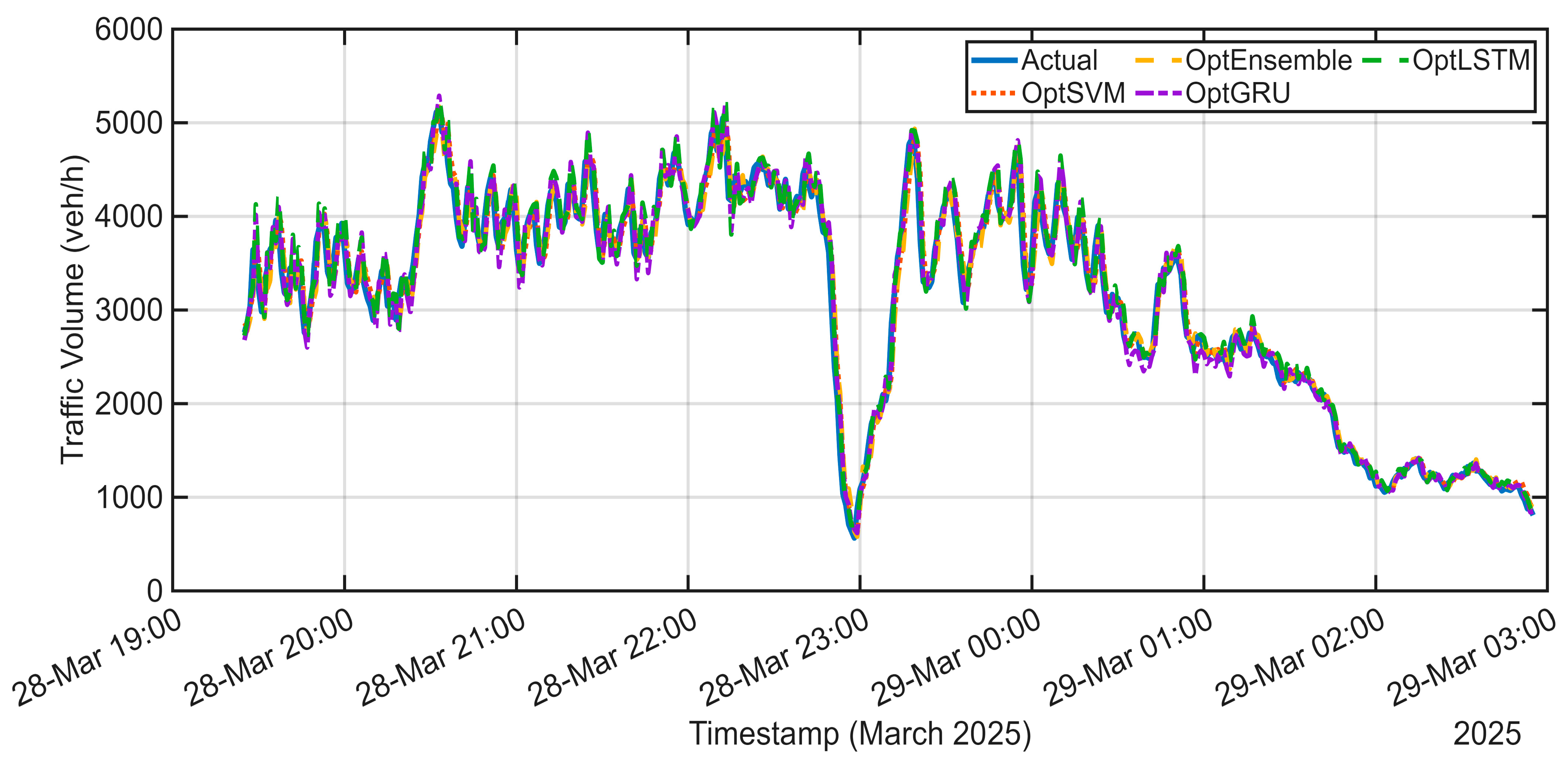
Figure 8 and Figure 9 present the full-range and zoomed-in temporal comparisons between the observed traffic volumes and the predictions generated by the optimized models. Compared with their baseline counterparts, the optimized configurations demonstrate a substantially improved ability to follow rapid variations in traffic demand, reproducing both peak intensities and sudden transitions in traffic volume with higher fidelity.

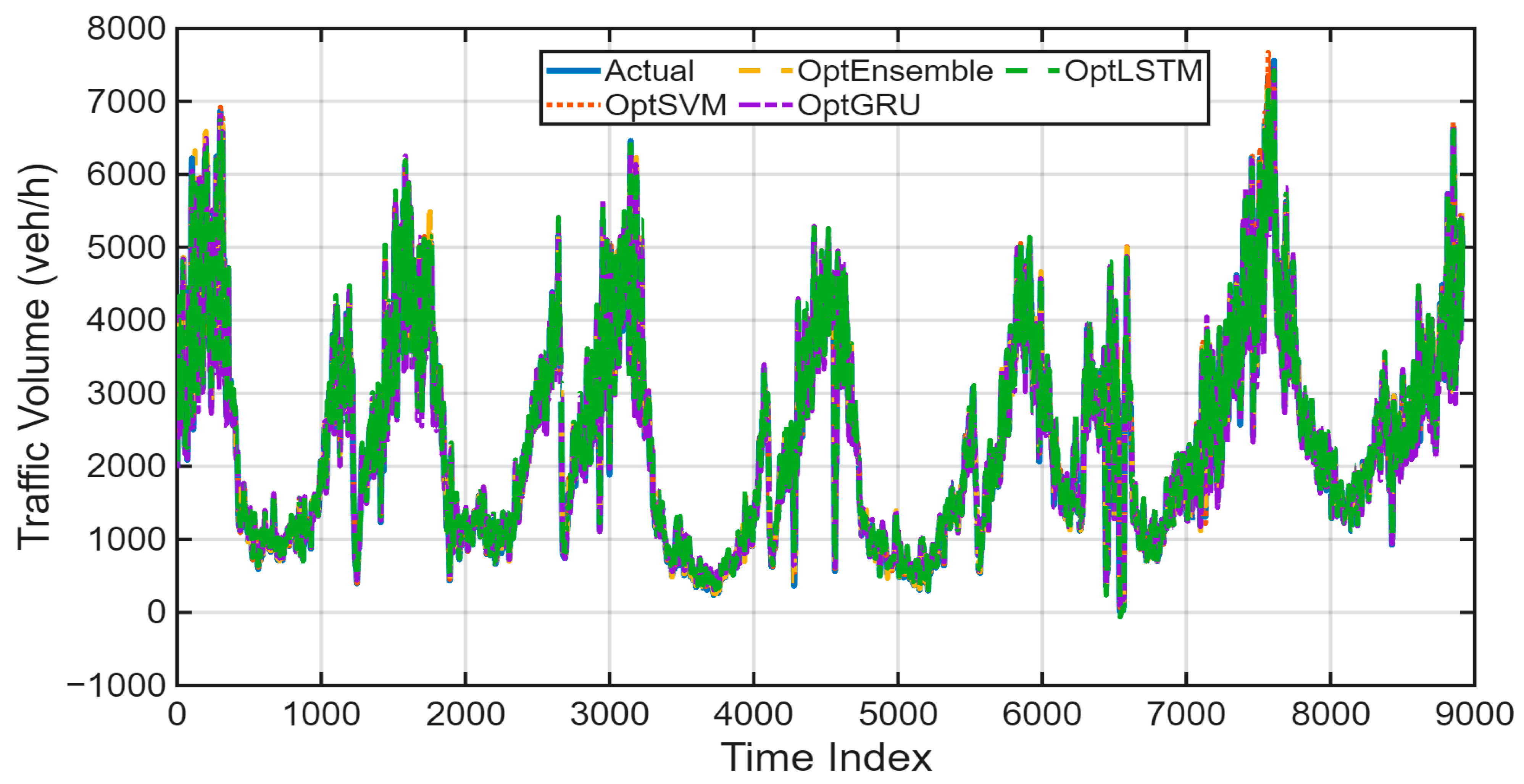
Figure 8 illustrates the full temporal evolution of traffic volume over the entire test horizon. All optimized models capture the dominant cyclical structure of traffic demand, including the recurrent peak–off-peak patterns that characterize daily urban traffic operations. The predicted trajectories closely follow the observed measurements across most of the timeline, indicating that the optimized models are capable of representing both long-term traffic trends and short-term fluctuations present in the dataset. This behavior is consistent with the improved quantitative performance reported in Table 2, where the optimized models achieve lower prediction errors compared with their baseline counterparts.

A clearer comparison between models becomes visible in the zoomed segment presented in Figure 9, which focuses on a short interval characterized by abrupt traffic variations. In this region, the optimized models are required to track a rapid drop in traffic volume followed by a sharp recovery. The optimized recurrent models, OptLSTM and OptGRU, exhibit the closest temporal alignment with the observed traffic signal. Both models respond effectively to the sudden congestion collapse and subsequent recovery phase, reproducing the steep decline and rebound with minimal lag and limited amplitude distortion. This behavior highlights the ability of recurrent architectures to capture complex temporal dependencies in traffic flow dynamics.

The optimized machine learning models, including OptSVM and OptEnsemble, also demonstrate noticeable improvements compared with their baseline counterparts. These models follow the overall traffic trend and reproduce the main peaks reasonably well; however, small deviations remain visible during the most abrupt transitions, particularly around the lowest traffic values in the zoomed interval. This suggests that while optimized classical models can approximate the general traffic pattern effectively, their ability to capture highly nonlinear temporal dynamics remains slightly more limited than that of recurrent deep learning architectures.

Overall, the visual analysis presented in Figure 8 and Figure 9 indicates that systematic hyperparameter optimization plays a critical role in enhancing prediction accuracy and temporal stability. The optimized models exhibit improved alignment with observed traffic volumes and reduced deviations during abrupt changes. Among them, the optimized deep learning models achieve the most consistent temporal tracking performance, reinforcing their suitability for short-term traffic forecasting and real-time intelligent transportation system applications in complex urban environments.

3.5. Stability and Residual Analysis

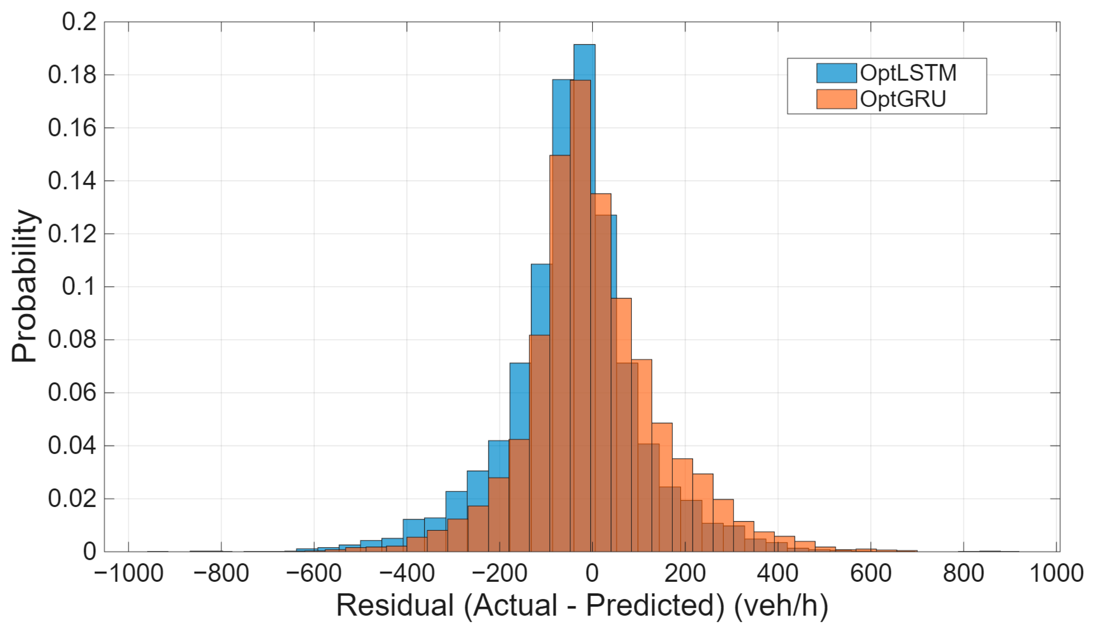
Figure 10 presents the residual histograms of the optimized LSTM and GRU models, where residuals are defined as the difference between the actual and predicted traffic volumes. Residual analysis was focused on these two models because they achieved the highest predictive accuracy and the most stable temporal performance among all evaluated approaches.

As shown in Figure 10, the residual distributions of both models are approximately centered around zero, indicating that prediction errors are generally balanced between overestimation and underestimation. Both distributions exhibit a concentrated peak near zero with gradually decreasing tails, which suggests that most prediction errors remain within a moderate range and that large deviations occur relatively infrequently.

A close comparison between the two histograms indicates similar overall error behavior for OptLSTM and OptGRU, confirming that both architectures provide comparable robustness and generalization capability. At the same time, the presence of residual tails extending in both positive and negative directions suggests that occasional larger prediction errors still occur under highly dynamic traffic conditions. Overall, the residual distributions support the conclusion that the optimized recurrent models achieve stable and largely unbiased prediction performance under real-world urban traffic conditions.

3.6. Key Insights and Practical Implications

The comparative evaluation highlights clear differences in model behavior and suitability for short-term traffic load prediction under real urban operating conditions. Regression-based ML models demonstrate reasonable performance under stable traffic patterns, with linear regression and ensemble methods effectively capturing overall demand trends. However, their ability to represent abrupt traffic transitions and nonlinear temporal dependencies remains limited, particularly during highly dynamic congestion phases.

On the other hand, DL models, specifically optimized LSTM and GRU architectures, exhibit superior capability in capturing both short-term fluctuations and longer-term temporal dependencies inherent in high-resolution traffic data. The temporal and residual analyses confirm that systematic hyperparameter optimization is essential for achieving stable, unbiased, and responsive predictions, especially during peak and transition periods. Notably, optimized GRU models achieve performance comparable to LSTM while maintaining lower architectural complexity, offering a practical trade-off between accuracy and computational efficiency.

From an operational perspective, the findings provide guidance for model selection in smart city traffic applications. Simpler models may be suitable for low-complexity or interpretability-driven scenarios, whereas optimized DL models are better suited for real-time traffic monitoring and adaptive traffic management where accuracy and temporal stability are critical. Overall, the results emphasize that data-driven model selection and systematic optimization play a more decisive role in predictive performance than model complexity alone, supporting reliable deployment of traffic prediction systems in sustainable and intelligent urban mobility frameworks.

In recent years, transformer-based and attention-driven architectures have demonstrated promising performance in time-series forecasting and traffic prediction tasks due to their ability to model long-range temporal dependencies without recurrent structures. Although such architectures were not included in the present comparative framework to maintain controlled experimental consistency across widely adopted ML and DL baselines, they represent a valuable direction for future research. Investigating transformer-based traffic load prediction under similar high-resolution urban settings may further extend the contextual understanding of model robustness and scalability.

In terms of computational requirements, conventional machine learning models (linear regression, regression tree, SVM, and ensemble methods) exhibit relatively low training complexity and complete model training within seconds to a few minutes on the current dataset. This computational efficiency makes them particularly attractive for deployment in resource-constrained traffic monitoring environments. In contrast, deep learning models require longer training times due to sequential processing and iterative epoch-based optimization. In the present experiments, the training of LSTM and GRU networks required several minutes depending on the selected hyperparameter configuration. Nevertheless, during inference all models generate predictions within milliseconds per sample, confirming their practical suitability for real-time intelligent transportation system (ITS) applications with one-minute temporal resolution.

4. Conclusions

This study contributes to the traffic forecasting literature by providing a systematic comparative evaluation of conventional machine learning and deep learning models using high-resolution real-world traffic data collected from a major urban roundabout in Jeddah, Saudi Arabia. The analysis examines baseline and optimized model configurations to assess predictive accuracy, temporal behavior, and robustness under realistic operating conditions.

The results indicate that conventional ML models, such as linear regression and ensemble approaches, provide competitive performance under relatively stable traffic patterns and offer advantages in terms of simplicity and interpretability. However, their ability to represent nonlinear dynamics and abrupt traffic transitions remains limited. In contrast, DL architectures, particularly LSTM and GRU models, demonstrate stronger capability in capturing complex temporal dependencies and rapid traffic fluctuations when applied to high-resolution data.

From an operational perspective, the findings highlight that predictive performance is strongly influenced by data characteristics and model configuration rather than model complexity alone. Careful comparative evaluation enables informed model selection that balances accuracy, robustness, and practical deployment considerations. In the context of Saudi Vision 2030 and the United Nations’ Sustainable Development Goal 11 (Sustainable Cities and Communities), the proposed evaluation framework supports data-driven traffic management strategies that enhance mobility efficiency, reduce congestion, and contribute to sustainable urban transportation systems. Furthermore, the variability-based regime analysis emphasizes that traffic prediction model selection should consider demand dynamics rather than relying solely on aggregate evaluation metrics. Overall, the results highlight that model effectiveness is highly sensitive to hyperparameter configuration and traffic dynamics rather than model complexity alone.

From a practical deployment perspective, computational efficiency also plays an important role in model selection. In the present experiments, conventional machine learning models completed training within seconds to a few minutes, making them suitable for operational environments with limited computational resources. Deep learning models required longer training times due to iterative optimization and sequential processing; however, once trained, all models produced predictions within milliseconds per sample. This confirms that both ML and DL approaches are computationally feasible for real-time intelligent transportation system (ITS) applications with one-minute temporal resolution.

It is also important to acknowledge the scope and limitations of the present study. The analysis is based on traffic data collected from a single urban roundabout in Jeddah, Saudi Arabia. While the results provide valuable insights into model behavior under realistic operational conditions, the findings may not directly generalize to other road network configurations or urban environments without further validation. Moreover, the inclusion of previousVolumePerHour reflects short-term temporal persistence in traffic flow and is commonly used in traffic forecasting studies. However, it may also act as a strong autoregressive predictor. A detailed feature importance or ablation analysis is therefore identified as a potential direction for future work.

Future work will extend this study by incorporating additional contextual variables such as weather conditions and special events, exploring multi-horizon forecasting, and evaluating the proposed framework across multiple intersections or corridor-level traffic networks. Incorporating spatial interactions through graph-based or hybrid architectures also represents a promising direction for improving scalability and capturing network-level traffic dynamics.

References

1. Manibardo, E.L.; Laña, I.; Del Ser, J. Deep Learning for Road Traffic Forecasting: Does It Make a Difference? IEEE Trans. Intell. Transp. Syst. 2022, 23, 6164–6188. [Google Scholar] [CrossRef]
2. Majumdar, S.; Subhani, M.M.; Roullier, B.; Anjum, A.; Zhu, R. Congestion Prediction for Smart Sustainable Cities Using IoT and Machine Learning Approaches. Sustain. Cities Soc. 2021, 64, 102500. [Google Scholar] [CrossRef]
3. Akhtar, M.; Moridpour, S. A Review of Traffic Congestion Prediction Using Artificial Intelligence. J. Adv. Transp. 2021, 2021, 8878011. [Google Scholar] [CrossRef]
4. United Nations. Transforming Our World: The 2030 Agenda for Sustainable Development; Resolution A/RES/70/1; United Nations: New York, NY, USA, 2015; Available online: https://sdgs.un.org/2030agenda (accessed on 19 March 2026).
5. Sun, S.; Zhang, C.; Yu, G. A Bayesian network approach to traffic flow forecasting. IEEE Trans. Intell. Transp. Syst. 2006, 7, 124–132. [Google Scholar] [CrossRef]
6. Tang, J.; Chen, X.; Hu, Z.; Zong, F.; Han, C.; Li, L. Traffic flow prediction based on combination of support vector machine and data denoising schemes. Physica A 2019, 534, 120642. [Google Scholar] [CrossRef]
7. Qiu, J.; Zhao, Y. Traffic prediction with data fusion and machine learning. Analytics 2025, 4, 12. [Google Scholar] [CrossRef]
8. Lin, G.; Lin, A.; Gu, D. Using Support Vector Regression and K-Nearest Neighbors for Short-Term Traffic Flow Prediction Based on Maximal Information Coefficient. Inf. Sci. 2022, 608, 517–531. [Google Scholar] [CrossRef]
9. Yi, Z.; Liu, X.C.; Markovic, N.; Phillips, J. Inferencing hourly traffic volume using data-driven machine learning and graph theory. Comput. Environ. Urban Syst. 2021, 85, 101548. [Google Scholar] [CrossRef]
10. Ou, J.; Li, J.; Wang, C.; Wang, Y.; Nie, Q. Building Trust for Traffic Flow Forecasting Components in Intelligent Transportation Systems via Interpretable Ensemble Learning. Digit. Transp. Saf. 2024, 3, 126–143. [Google Scholar] [CrossRef]
11. Barredo Arrieta, A.; Laña, I.; Del Ser, J. What Lies Beneath: A Note on the Explainability of Black-Box Machine Learning Models for Road Traffic Forecasting. In Proceedings of the 2019 IEEE Intelligent Transportation Systems Conference (ITSC), Auckland, New Zealand, 27–30 October 2019; pp. 2232–2237. [Google Scholar] [CrossRef]
12. Kim, M.; Lee, D. Why uncertainty in deep learning for traffic flow prediction is needed. Sustainability 2023, 15, 16204. [Google Scholar] [CrossRef]
13. Abdullah, S.M.; Periyasamy, M.; Kamaludeen, N.A.; Towfek, S.K.; Marappan, R.; Kidambi Raju, S.; Alharbi, A.H.; Khafaga, D.S. Optimizing traffic flow in smart cities: Soft GRU-based recurrent neural networks for enhanced congestion prediction using deep learning. Sustainability 2023, 15, 5949. [Google Scholar] [CrossRef]
14. Topilin, I.; Jiang, J.; Feofilova, A.; Beskopylny, N. Traffic flow prediction via a hybrid CPO-CNN-LSTM-attention architecture. Smart Cities 2025, 8, 148. [Google Scholar] [CrossRef]
15. Zhang, Y.; Wang, X.; Xie, J.; Bai, Y. Comparative Analysis of Deep-Learning-Based Models for Hourly Bus Passenger Flow Forecasting. Transportation 2024, 51, 1759–1784. [Google Scholar] [CrossRef]
16. Zhang, J.; Sha, J.; Zhang, C.; Zhang, Y. A CNN-LSTM-GRU hybrid model for spatiotemporal highway traffic flow prediction. Systems 2025, 13, 765. [Google Scholar] [CrossRef]
17. Liu, R.; Shin, S.Y. A review of traffic flow prediction methods in intelligent transportation system construction. Appl. Sci. 2025, 15, 3866. [Google Scholar] [CrossRef]
18. Mystakidis, A.; Koukaras, P.; Tjortjis, C. Advances in traffic congestion prediction: An overview of emerging techniques and methods. Smart Cities 2025, 8, 25. [Google Scholar] [CrossRef]
19. Tsalikidis, N.; Mystakidis, A.; Koukaras, P.; Ivaškevičius, M.; Morkūnaitė, L.; Ioannidis, D.; Fokaides, P.A.; Tjortjis, C.; Tzovaras, D. Urban traffic congestion prediction: A multi-step approach utilizing sensor data and weather information. Smart Cities 2024, 7, 233–253. [Google Scholar] [CrossRef]
20. Vlahogianni, E.I.; Karlaftis, M.G.; Golias, J.C. Short-term traffic forecasting: Where we are and where we’re going. Transp. Res. Part C Emerg. Technol. 2014, 43, 3–19. [Google Scholar] [CrossRef]
21. Guo, S.; Lin, Y.; Feng, N.; Song, C.; Wan, H. Attention based spatial-temporal graph convolutional networks for traffic flow forecasting. In Proceedings of the AAAI Conference on Artificial Intelligence, Honolulu, HI, USA, 27 January–1 February 2019; Volume 33, pp. 922–929. [Google Scholar] [CrossRef]
22. Dong, Z.; Yu, S.; Shen, Y. Multi-scale dynamic hypergraph convolutional network for traffic flow forecasting. J. Shanghai Jiaotong Univ. (Sci.) 2025, 30, 880–888. [Google Scholar] [CrossRef]
Figure 1. Load Traffic Prediction Overall Framework.
Smartcities 09 00056 g001
Figure 2. Diurnal pattern of traffic volume at the Earth Globe Roundabout.
Smartcities 09 00056 g002
Figure 3. Diurnal pattern of vehicle delay at the Earth Globe Roundabout.
Smartcities 09 00056 g003
Figure 4. RMSE of the baseline and optimized prediction models.
Smartcities 09 00056 g004
Figure 5. Variability-based regime definition derived from the test dataset: (a) rolling standard deviation of traffic volume computed using a 30-min window with percentile-based thresholds indicating high- and low-variability regimes; (b) distribution of variability scores with vertical dashed lines marking the 30th and 70th percentile thresholds used to classify low- and high-variability conditions.
Smartcities 09 00056 g005
Figure 6. Full-range prediction results of the baseline models.
Smartcities 09 00056 g006
Figure 7. Zoom-range prediction results of the baseline models.
Smartcities 09 00056 g007
Figure 8. Full-range prediction results of the optimized models.
Smartcities 09 00056 g008
Figure 9. Zoom-range prediction results of the optimized models.
Smartcities 09 00056 g009
Figure 10. Residuals of optimized DL-based prediction models.
Smartcities 09 00056 g010