Performance Analysis of Different Borehole Heat Exchanger Configurations: A Case Study in NW Italy

Highlights

What are the main findings?

• A good knowledge of the underground parameters and of the aquifer characteristics are essential in the design of borehole heat exchangers as part of a shallow geothermal plant integrated in a district heating and cooling grid.
• Borehole heat exchangers with a coaxial configuration outperform double U pipes in terms of energy efficiency, especially during intermittent operation modes of the geothermal heating system.

What is the implication of the main finding?

• Proper design of a shallow geothermal plant can potentially reduce the cost of drilling boreholes and make the installation easier on site, also improving the sustainability of urban environments.
• A geothermal-based district heating and cooling grid can be combined with other renewable energies, achieving the best thermal energy performance, improving smart energy systems, and the decarbonisation of the building sector.

Abstract

The central role of heating and cooling in energy transition has been recognised in recent years, especially with geopolitical developments since February 2022 which demand an acceleration in deploying local energy sources to increase the resilience of the energy sector. Geothermal energy is a promising and vital option to optimize heating and cooling systems, promoting sustainability of urban environments. To this end, a proper design is of paramount importance to guarantee the energy performance of the whole system. This work deals with the optimization of the technical and geometrical characteristics of borehole heat exchangers (BHEs) as part of a shallow geothermal plant that is assumed to be integrated in an already operating gas-fired DH grid. Thermal performances of three different configurations were analysed according to the geological information that revealed an aquifer at −36 m overlying a poorly permeable marly succession. Numerical simulations validated the geological, hydrogeological, and thermo-physical models by back-analysing the experimental results of a thermal response test (TRT) on a pilot 150 m deep BHE. Five-year simulations were then performed to compare 150 m and 36 m polyethylene 2U, and 36 m steel coaxial BHEs. The coaxial configuration shows the best performance both in terms of specific power (74.51 W/m) and borehole thermal resistance (0.02 mK/W). Outcomes of the study confirm that coupling the best geological and technical parameters ensure the best energy performance and economic sustainability.

1. Introduction

The energy crisis of the last three years has led governments to put in place short- and long-term measures aimed at shielding consumers from the direct impact of the rising energy prices across Europe and to counteract the continuous economic volatility [1]. The pressure is high for finding solutions to reduce energy imports and fight against climate change impacts. As described in the last report on climate change by the Intergovernmental Panel on Climate Change (IPCC, [2]), urgent and faster actions are needed to mitigate global warming and limit the temperature increase to 1.5 °C above pre-industrial levels [3]. The geopolitical situation requires new approaches mainly for the decarbonisation of the heating and cooling (H&C) sector, which is still responsible for almost half of the final energy consumption in Europe. Moreover, H&C significantly depends on energy imports, above all, fossil fuels [4,5]. Low carbon sources, such as geothermal energy, represent a vital option to produce cleaner energy and substantially decrease its consumption and cost, especially when integrated into district heating and cooling (DHC) grids [3,4,5,6]. In this way, the direct heat exchange can strongly facilitate decarbonisation by supplying energy with a high level of flexibility [7].

However, due to a fragmented regulatory framework across Europe, geothermal energy still plays a minor role in the European H&C sector, slowing down its economic development [6,8,9]. Further implementation of this technology represents an urgent challenge to reduce energy import.

The recent multiple crises have led to an increased interest in using geothermal energy in DHC to substitute fossil fuels, especially natural gas. However, due to shortcomings in the market development efforts in the past years, services needed for the rollout of DHC in Europe are limited and require significant ramp-up periods [6]. One of the most important and recent initiatives aimed at increasing the use of renewable energy sources is the “European Parliament resolution 2023/2111(INI) on geothermal energy”. This reveals the paramount importance of shallow geothermal technologies such as ground-source heat pumps (GSHP), which represent one of the most common applications for space heating and cooling [10].

According to [11], thermal interferences between boreholes due to a dense installation of shallow geothermal systems may cause the ground to be overexploited as well as limit the technical performance of the whole system. At the same time, the technical potential should be defined at a regional scale, evaluating the area in which BHEs can provide higher thermal potential and their impact on the ground. However, thermal performances of BHEs are linked to a number of factors such as the grout used in sealing the borehole, which withstands mechanical stress and environmental impacts, to the cyclic freeze–thaw loads [11], the thermal characteristics of the geological formations of interest, and the groundwater flow.

Different methodologies are discussed in the literature to optimize the thermal performance of BHEs, also comparing those considered as the best performing. Among these, [12] showed the results of different flow and heat transport simulations to evaluate the impact of different parameters on the operation of H&C systems. They demonstrated how BHE length as well as grouts and heat carrier fluid can influence ground source heat pump (GSHP) operation. A similar analysis was conducted by [13], who compared the thermal and hydraulic parameters together with the maximum operational depth of coaxial, single U, and double U pipes for shallow to deep BHEs. Energy performances comparing coaxial and double U pipes were also evaluated in [14,15]. In particular, in [14] the short- and long-term operation of the different pipe geometries were analysed, and the simulation revealed how the coaxial configuration allowed for a better thermal performance due to the higher thermal capacitance of the heat carrier fluid and the lower borehole thermal resistance. Numerical simulations were used by [16] to investigate the effect of different design parameters such as single U, double U, and cross U pipe for small-diameter boreholes, observing that the thermal performance of the system is enhanced by passing from the laminar to the turbulent regime and by increasing the volume in which the heat transfer fluid can flow. Moreover, other works focused on the comparison between coaxial and double U pipes, also evaluating their performances during intermittent operation modes [16,17,18,19,20]. However, most of these studies did not focus on optimizing the length of the BHE according to the geological and hydrogeological model of the site based on a detailed geothermal characterization, but they consider underground as an isotropic and homogenous medium. The influence of site characteristics such as subsurface and groundwater characteristics on BHE thermal performances were instead investigated by [21,22] through numerical simulations, employing steady state conditions but without considering the influence of the groundwater advection.

This study deals with the comparison of three geothermal BHE configurations aimed at providing space heating and cooling, in order to evaluate their thermal performance according to the local hydrogeological setting. The test site is located in Nizza Monferrato, Piedmont (NW Italy).

In particular, geological data served to set up a thermo-hydrogeological conceptual model which was validated by back-analysing a thermal response test (TRT) realised on a 150-meter pilot BHE. The resulting numerical model was then used to simulate five-year operation of 150 m and 36 m polyethylene 2U, and 36 m steel coaxial BHE. Thermal performance was analysed according to the specific power provided by each configuration and to their borehole thermal resistance.

Unlike previous works, the comparison of different borehole configurations evaluating their thermal performance based on specific geological, hydrogeological, and thermo-physical parameters of the underground soils is the innovative core of this work. Knowing the detailed hydrogeological conditions allows understanding of how the hydrodynamic characteristics of the groundwater can significantly increase the thermal efficiency, avoiding deeper and more expensive drillings.

2. Geological Setting

The investigated area (Figure 1) is in the municipality of Nizza Monferrato (NW Italy), about 70 km from Turin. It is located in the upper Monferrato, one of the tectono-sedimentary domains of the Tertiary Piedmont Basin (TPB), a terrigenous Upper Miocene to Pliocene succession originating in the Alpine retro-foreland after the mid-Eocene continental collision between the Adriatic promontory and the European plate [23]. The TPB is a >4 km thick marine sedimentary succession juxtaposed to the Alpine and Apennine metamorphic tectonic units [23,24]. It covers the boundary between the Alpine and Apennine thrust belts and can be considered as a crustal piggy-back basin of the Miocene Apennine belt [25]. In particular, the Monferrato area represents the north-western part of the Apennines together with the Turin Hills [26,27]; it consists of the folded marine Tertiary formations and overlies the Plio-Quaternary thrust belt which divides the TPB from the Mesozoic and Cenozoic geological units underneath the fluvial lithologies of the Po Plain [25].

The test site (Figure 1) is mainly characterized by a NW–SW faulting system [28] and, in particular, the Nizza Monferrato area mainly consists of the following Pliocenic and Messinian deposits [27,29]:

• “Marne di Sant’Agata Fossili” (Tortonian/Lower Messinian), bioturbated clayey to calcareous foraminifers-rich marl sediments, showing a gradual transition toward the top into a rhythmic alternation of marls and organic-rich, extremely laminated mudstones (VGS₃, in Figure 1);
• “Membro di Nizza Monferrato” (Messinian), belonging to the “Gessoso-Solfifera” geological unit mainly composed of clays, silts, and subordinate sandstones with a variable colour including dark yellow, grey, cream-white, and purple, in which a primary laminated microcrystalline gypsum bed is recognizable (CCS, in Figure 1);
• “Conglomerati di Cassano-Spinola” (Upper Messinian), a succession of sandy and pelitic layers bordered at the top and bottom by irregular erosional surfaces [30] following in discontinuity the “Gessoso-Solfifera” (CCS, in Figure 1);
• “Villafranchiano” (Plio-Pleistocene), a sedimentary succession represented by transgressive-regressive deposits, the base of which consist of deep-sea clayey sediments (“Argille Azzurre” Unit) followed by sands of marginal marine environment (“Sabbie di Asti”) [30] (FAA, in Figure 1);
• “Quaternary succession” (Holocene–present), consisting of sandy-gravelly and silty-sandy fluvial deposits which overlie all the stratigraphic succession; it is present in the shallower 30 m (MEA₃ and CMT₃, in Figure 1).

Figure 1. Geological sketch map with the pilot BHE location represented by a red star (modified after “Carta Geologica d’Italia, Foglio 194 Acqui Terme” by “Progetto CARG” of ISPRA [29]). The A–A’ cross section represents the area in which the geophysical surveys were conducted; green points represent field thermal conductivity measures (see next sections).

Figure 1. Geological sketch map with the pilot BHE location represented by a red star (modified after “Carta Geologica d’Italia, Foglio 194 Acqui Terme” by “Progetto CARG” of ISPRA [29]). The A–A’ cross section represents the area in which the geophysical surveys were conducted; green points represent field thermal conductivity measures (see next sections).

Available geophysical data allowed inferring the subsurface characteristics based on the resistivity and chargeability obtained by an electrical resistivity tomography (ERT), realised close to the investigated area. These properties allowed highlighting of the relevant geological formations in order to set up the thermo-hydrogeological conceptual model relevant for geothermal applications as commonly described in the literature [31,32,33,34,35]. The ERT was performed by means of 80 stainless steel electrodes with 6 m spacing, a dipole-dipole array configuration for the acquisition with a total of 2310 potential measurements (Figure 2). The adopted configuration allowed a resolution of about 3 m both in the x and depth directions (i.e., half the adopted electrodes spacing). Along the investigated line no particular topography was present; therefore, no topographic correction was applied to the data.

Tomographies show the presence of a shallow (5 to 10 m) coverage with low resistivity (10–40 Ohm.m) and low chargeability (<1 ms) values. This coverage can be related to the presence of anthropic landfill, generally correlated with low-water-content sands. Below this layer there is a thick (20–30 m), low-resistivity (generally < 30 Ohm.m), high-chargeability (>7 ms) formation, potentially associated with the presence of saturated sandy-silty alluvial deposits with localized clay lenses (Holocene alluvial deposits). In particular, the evidence of isolated high chargeability zones (>10 ms) could reflect the presence of areas with significant silty content. This formation overlays a generally medium-high resistivity (around 80 Ohm.m) and a medium-low chargeability (around 5 ms) formation consisting of compacted silts and clays (“Gessoso-Solfifera”). Within this deep formation, a zone showing low resistivity (< 10 Ohm.m) and high chargeability (>6 ms) is potentially correlated to high clay content.

3. Materials and Methods

Specific field tests were conducted to integrate the available geological information and further characterize the conceptual model with both thermal and hydrogeological data. Numerical simulations were first carried out to validate the conceptual model through a back-analysis of the TRT. In a second step, the validated numerical model was used to simulate the long-term operation of different borehole configurations having the following characteristics (

Table 1. BHE characteristics. Keys: L is the BHE length; D is the BHE diameter; d_in and d_out are the inner and outer pipe diameters; b_in and b_out represent the inner and outer pipe thicknesses; and λ_in and λ_out are the inner and outer pipe thermal conductivities. Shank spacing refers to the space between the outer and the inner pipe centres, only for 2U geometries. Concerning coaxial configurations: subscript “in” refers to the central polyethylene pipe, while subscript “out” to the stainless steel outer pipe.

BHE Configuration	L (m)	din (m)	bin (m)	dout (m)	bout (m)	D (m)	λin (W × m−1 K−1)	λout (W × m−1 K−1)	Shank Spacing (m)	Grout Sealing Wall BHE
Double U (PE100 SDR11)	150	0.026	-	0.032	0.0029	0.152	-	0.42	0.12	Bentonite
Double U (PE100 SDR11)	36	0.026	-	0.032	0.0029	0.152	-	0.42	0.12	Bentonite
Coaxial	36	0.025	0.0023	0.065	0.0080	0.178	0.42	52	-	Bentonite

):

• 2U150 m: polyethylene double U pipe with a depth of 150 m, which corresponds to the pilot borehole (borehole diameter: 0.152 m; pipe diameter: 0.032 m; pipe wall thickness: 0.0029 m);
• 2U36 m: polyethylene double U pipe with a depth of 36 m, in light of the base of the aquifer highlighted by the pilot drilling (borehole diameter: 0.152 m; pipe diameter: 0.032 m; pipe wall thickness; 0.0029 m);
• Coax 36 m: coaxial configuration with stainless steel outer casing (outer diameter: 0.061 m; wall thickness: 0.008 m) and polyethylene inner pipe (outer diameter: 0.025 m; wall thickness: 0.0023 m) with a depth of 36 m.

3.1. Field Tests

Thermal conductivity measurements were carried out on the outcropping geological formations in the neighbouring of the investigated area (Figure 1). The adopted device was a KD2Pro (Decagon Device), a commercial thermal property analyser which conforms to IEEE Standard 442-1981 and to the ASTM Standard D5334-00, and is based on a proprietary algorithm [36]. This device consists of four needle probes of which the RK-1 has been assessed as the most appropriate one to be inserted in the investigated materials (0 cm long, 3.9 mm diameter, with an accuracy of ±10%).

Moreover, a pilot borehole (diameter 0.152 m) was drilled down to 150 m below ground level (b.g.l.) and equipped with a double U (2U) polyethylene pipe (outer pipe diameter 0.032 m). The stratigraphy deduced by the drilling confirmed the geological model described in the previous section and highlighted the presence of a sandy aquifer in the first 36 m b.g.l.

A thermal response test (TRT) investigating a preliminary vertical borehole 150 m in depth, was further conducted with a flow rate of 0.45 l/s and an average power of 6.3 kW over 72 h. The test followed the same characteristics as reported in [37,38]; it provided subsurface thermal parameters such as thermal conductivity and borehole thermal resistance, aimed at evaluating the heat transfer mechanism with greater accuracy. Equation (1), developed by [39], was used to accurately defined the results obtained from the TRT:

$$\mathrm{Tf}\left(\mathrm{t}\right)={\displaystyle \frac{\mathrm{q}}{4\mathrm{\pi }\mathrm{\lambda }}}\ast \left(\ln {\displaystyle \frac{4\mathsf{\alpha }\mathrm{t}}{{\mathrm{r}}^2}}-\mathsf{\gamma }\right)+\mathrm{q}\ast \mathrm{Rb}+\mathrm{Tg}$$

(1)

where

• Tf(t) is the average fluid temperature (T_in and T_out) depending on the test time, expressed in °C.
• q is the injected power in the unit of time and depth, expressed in W/m and is equal to Q/H (H is the drilling depth), in which Q is the injected power in the unit of time, expressed in W.
• λ is the ground thermal conductivity, expressed in W/m/K.
• γ is the Eulero constant, equal to 0.5772.
• α is the thermal diffusivity, expressed in m²/s.
• t is the test time, expressed in s.
• r is the borehole radius, expressed in m.
• Rb is the borehole thermal resistance, expressed in K/(W/m).
• Tg is the undisturbed temperature, expressed in °C.

3.2. Numerical Simulations

Numerical simulations were performed with FeFlow^®, a finite element commercial software for groundwater and porous media modelling with a specific tool for BHE simulations. The geometrical model consists of a 3D volume 50 × 50 × 200 m, spatially discretized into 69,264 triangular prism elements and 37,200 nodes. The meshing methodology followed the same procedure as in [37,38], and [40] but better refining the mesh thanks to the updated features of the 8.1 version. A point gradation of 2 was used, as well as 0.2 m for polygons and the point target size, and a check for obtuse angles and triangles violating the Delaunay criterion was also conducted. On each active node of the mesh, the algebraic MultiGrid Solver (SAMG) was used.

In order to validate the conceptual model, a trial and error back-analysis technique was used to fit the numerical data to the experimental results obtained from the TRT test (3.1). The Al Khoury approach [41], a fully transient method which provides higher accuracy for short-term predictions, was applied to simulate the 72 h TRT test. It consists of a specific time step typical for transient groundwater conditions, and it is based on differential equations [42].

Aimed at better defining the hydraulic conditions, the 1st kind flow boundary conditions (BC) were set on both sides of the 3D model; this allows reproducing the hydraulic gradient equal to about 0.3%, as well as a S/N groundwater flow direction. Concerning the thermo-technical model, the 4th kind boundary condition which defines BHE properties was applied to 6.3 kW of constant thermal power for 72 h. During the back analysis of the TRT, ground parameters such as thermal conductivity, hydraulic conductivity and hydraulic gradient were gradually changed to get closer to the results obtained from the TRT and then to real conditions. These properties represent those which affect the heat transfer more, playing an important role in handling the inlet and outlet temperatures during the BHE operation. This approach was fundamental in refining the previous collected information, well defining the geological, hydrogeological, and thermo-physical models. Furthermore, the undisturbed ground temperature was also configured to match the profile, measured before the TRT.

In addition, to better calculate the heat transfer during the numerical simulation, another key parameter, the borehole thermal resistance, was taken into account. Borehole thermal resistance was calculated along the depth of the BHE through Equation (2), using average fluid and wall temperature inferred from the numerical model:

$$Rb={\displaystyle \frac{Tf-Tb}{q}}$$

(2)

where

• Tf is the average fluid temperature (T_in and T_out) depending on the test time, expressed in °C.
• q is the injected power in the unit of time and depth, expressed in W/m and is equal to Q/H (H is the drilling depth), in which Q is the injected power in the unit of time, expressed in W.
• Tb is the borehole wall temperature expressed in °C.
• Rb is the borehole thermal resistance, expressed in m K W⁻¹.

All these steps were needed to validate the final geothermal model, which was then used as a basis for the long-term simulations of the three different BHE configurations. Unlike the previous simulations conducted by back-analysing the TRT, in this case the quasi-stationary method by Claesson & Eskilson [43] was applied. This approach is adopted when long-term simulations with less frequent and less steep inflow temperature changes occur. It provides a reasonable accuracy at lower computational cost and assumes a local thermal equilibrium between all the elements of the BHE (pipes, grout, and ground) at any time of the simulation [42]. In this case, the computed heat transfer coefficient, calculated from the geometrical information and the thermal conductivities of the different BHE parts, was used. For these long-term numerical simulations, the different BHEs considered consist of typical characteristics used in the Italian market as shown in Table 1. Unlike the previous numerical simulations of the TRT test, the operation of each BHE configuration was simulated by assigning an inlet temperature of 0 °C for 12 h on- and off- daily cycles, over five-year simulations.

4. Results

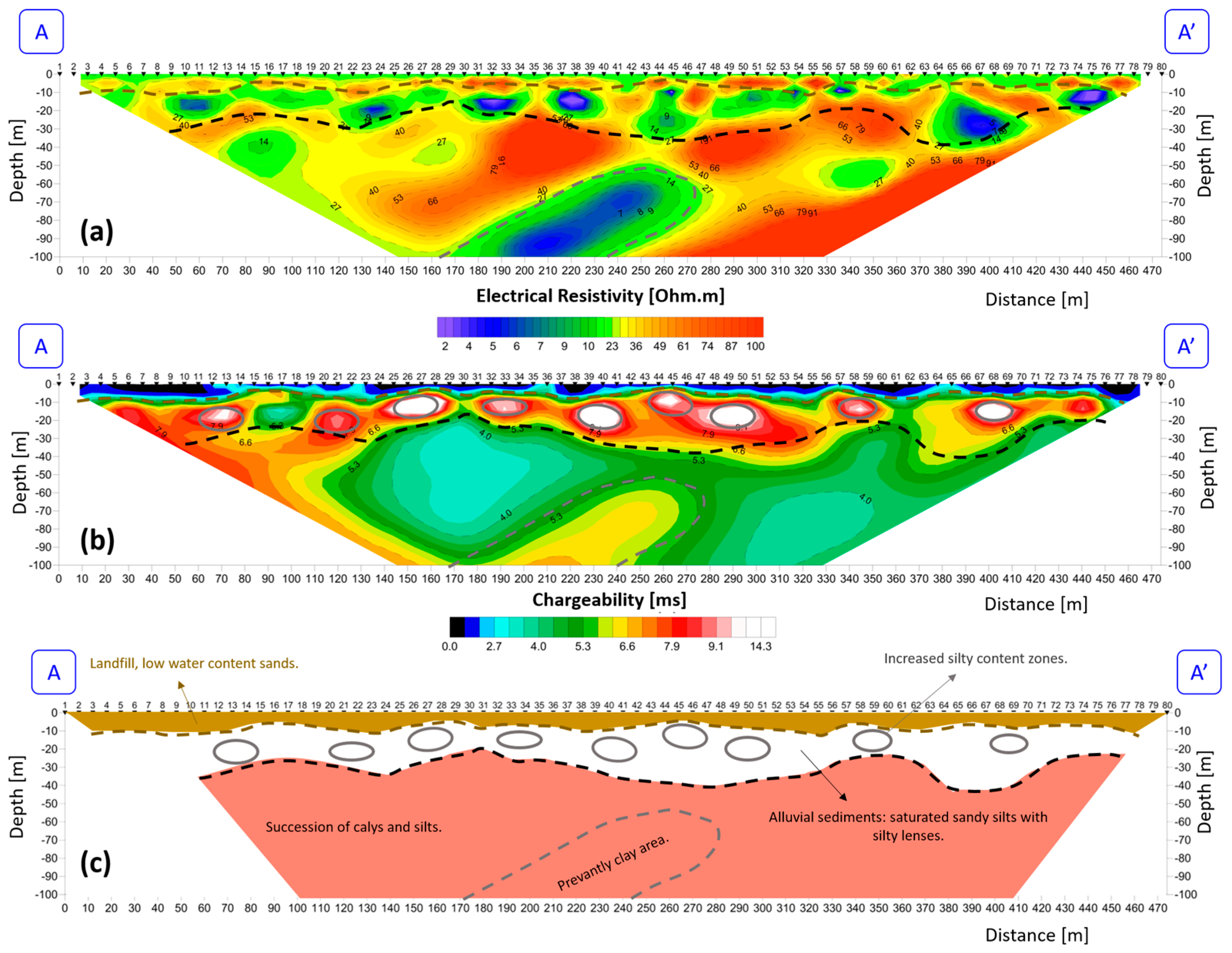
4.1. Thermo-Geological Conceptual Model

Collected geological data enabled identifying a multi-aquifer system that can reach a maximum thickness of about 36 m. This system is generally characterized by shallower deposits with a discrete to good hydraulic conductivity (e.g., Holocenic alluvial deposits) ranging from 10⁻⁴ to 10⁻⁵ m s⁻¹, followed by deeper medium to low porosity deposits such as the “Gessoso-Solfifera” (10⁻⁶ m s⁻¹) and the “Marne di Sant’Agata Fossili” (10⁻⁷ to 10⁻⁸ m s⁻¹) formations. Thermal conductivity measurements highlighted low values for alluvial sediments (λ = 0.65 W m⁻¹ K⁻¹), sandy and pelitic succession (λ = 0.66 W m⁻¹ K⁻¹), silts, clays, and clayey marls (λ = 0.79 W m⁻¹ K⁻¹). These low thermal conductivity values can be mainly ascribed to several factors such as the needle probe not being well inserted due to coarse-grained sediments in the finer matrix that hinder its insertion at depth, or due to alteration or weathering typical of outcropping deposits. However, the thermal conductivity data obtained can be considered typical of sediments when dry conditions occurred.

The undisturbed underground temperature was measured with PT100 sensors inside the BHE through a cable containing sensors placed at specific depths, as shown in

Table 2. Temperature profile measured in the pilot BHE.

Depth b.g.l. (m)	Lithology	Temperature (°C)
10	Sands	13.9
30	Sands and saturated silts	14.2
60	Silts and clays	14.6
100	Marls	15.6
120	Marls	16.2
150	Marls	16.7

. The PT100 sensors were placed some days after its completion and just before conducting the TRT by recording inlet and outlet temperatures of the heat carrier fluid circulating inside the pipe, as proposed by [44]. Once starting the TRT, after approximately 15 min of fluid circulation, the temperature fluctuations evened out and the estimate of the average undisturbed ground temperature was about 14 °C. This value is lower than those measured through PT100 sensors because it represents an average along the entire length of the borehole. The temperature profile in Table 2 was obtained by using thermal sensors, thus defining the final thermogeological model of the investigated area.

Inlet and outlet temperatures of the heat carrier fluid tend to stabilize 10–15 h after starting TRT, reaching 27.3 °C (inlet) and 24.0 °C (outlet) at the end of the test, as shown in Figure 3. These values were useful to calculate both the average thermal conductivity (1.94 W m⁻¹K⁻¹) and the average borehole thermal resistance R_b (0.07 m K W⁻¹) via the common infinite line source analytical model as reported in [36]. The TRT outputs only one value of both the thermal conductivity and the borehole thermal resistance, as the average values of the subsurface and of the borehole, respectively, without considering differences in lithologies, ground water, or grouting. As widely investigated in previous studies [36,45], thermal properties of soils strongly depend on their mineralogical composition, porosity, and density, as well as on hydrogeological characteristics.

The knowledge of these specific parameters is of paramount importance to evaluate the heat transfer from each specific layer. To this aim, results from the back-analysis of the TRT were helpful to validate all the ground parameters at depth. The valid agreement between experimental and numerical results of the TRT testifies an accurate calibration of the thermogeological model, highlighting that the model can reliably reproduce heat transfer processes occurring in the subsurface when the geothermal system is operating. This is further verified by estimating the mean temperature (green continuous lines) using a 2% confidence interval (green dashed lines) of the average temperature curve.

Data collected from the literature, stratigraphic well logs, and site-specific tests, as well as from back-analysis of the TRT, allowed refining of the final thermogeological model as depicted in Figure 4 and in

Table 3. Geological, hydro-geological, and thermo-physical characteristics, as revealed by preliminary field surveys and information from the literature. Keys: λs is the soil thermal conductivity; Φ is the porosity; K is the hydraulic conductivity along X, Y, and Z directions; and T is the average undisturbed ground temperature based on temperature data from Table 2.

Depth (m)	Lithology	λs (W × m−1 K−1)	Φ	Kxx (m/s)	Kyy (m/s)	Kzz (m/s)	T (°C)
0–9	Sands	0.48	0.40	1.00 × 10−4	1.00 × 10−4	1.00 × 10−5	15.2
9–36	Sands and saturate silts	2.58	0.30	5.00 × 10−5	5.00 × 10−5	5.00 × 10−6	15.2
36–113	Silts and clays	2.56	0.45	1.00 × 10−6	1.00 × 10−6	1.00 × 10−7	15.2
113–150	Marls	2.46	0.20	1.00 × 10−7	1.00 × 10−7	1.00 × 10−8	15.2

.

Below a few meters of a sandy quaternary cover, the alluvial deposits host a discrete groundwater reservoir until a depth of about 36 m b.g.l. Between −36 and −113 m, a layer made by silts and clays, probably related to the “Gessoso-Solfifera” formation is characterized by a certain soil moisture but without a significant groundwater circulation. The deepest part up to 150 m depth consists of marly deposits probably refers to the “Marne di Sant’Agata Fossili” formation characterized by a very low permeability. For all these deposits, the thermal conductivity shows interesting values at about 2.5 W m⁻¹ K⁻¹.

4.2. Comparison of Different BHE Configurations

Results from numerical simulations comparing three different BHEs configurations during on- and off- cycles of 12 h each over five years are summarized in Figure 5 and Figure 6.

Figure 5 shows the specific thermal power [W/m] which can be extracted at the end of each on-cycle from the three BHEs over the first six months of the five-year simulation; these months were chosen as a reference slot to represent typical heating in the investigated area. As shown in Figure 5, the performance of the three BHEs are similar showing a quite abrupt decrease at the very beginning of the test and then stabilizing, respectively, at about 79.32 W/m for the Coax 36 m, 58.29 W/m for the 2U 36 m, and 46.24 W/m for the 2U 150 m at the end of the first six months.

On the other hand, Figure 6 represents the last 48 h of the fifth year of simulation, showing what is the specific power from each BHEs after each off- and on-cycle.

The two time slots at 43764 and 43788 as shown in Figure 6 refer to the specific power (W/m) at the 12th hour of each on-cycle after a 12 h off-cycle. In these cases, the specific thermal power of each BHE configuration reaches a very high value at 220 W/m, which only means the power required for switching on the plant, then they stabilize to the right value depending on the thermo-technical characteristics of each BHE.

The results obtained allow three main situations to be highlighted (

Table 4. Comparison of specific power [W/m] and borehole thermal resistance [m K W⁻] between the three different BHE configurations at step 5172 h.

BHE Type	Power 0–36 m [W]	Specific Power [W m−1]	Rb [m K W−1]
2U 150 m	1869.63	45.26	0.085
2U 36 m	2084.05	57.89	0.081
Coax 36 m	2839.88	78.89	0.020

; Figure 5 and Figure 6):

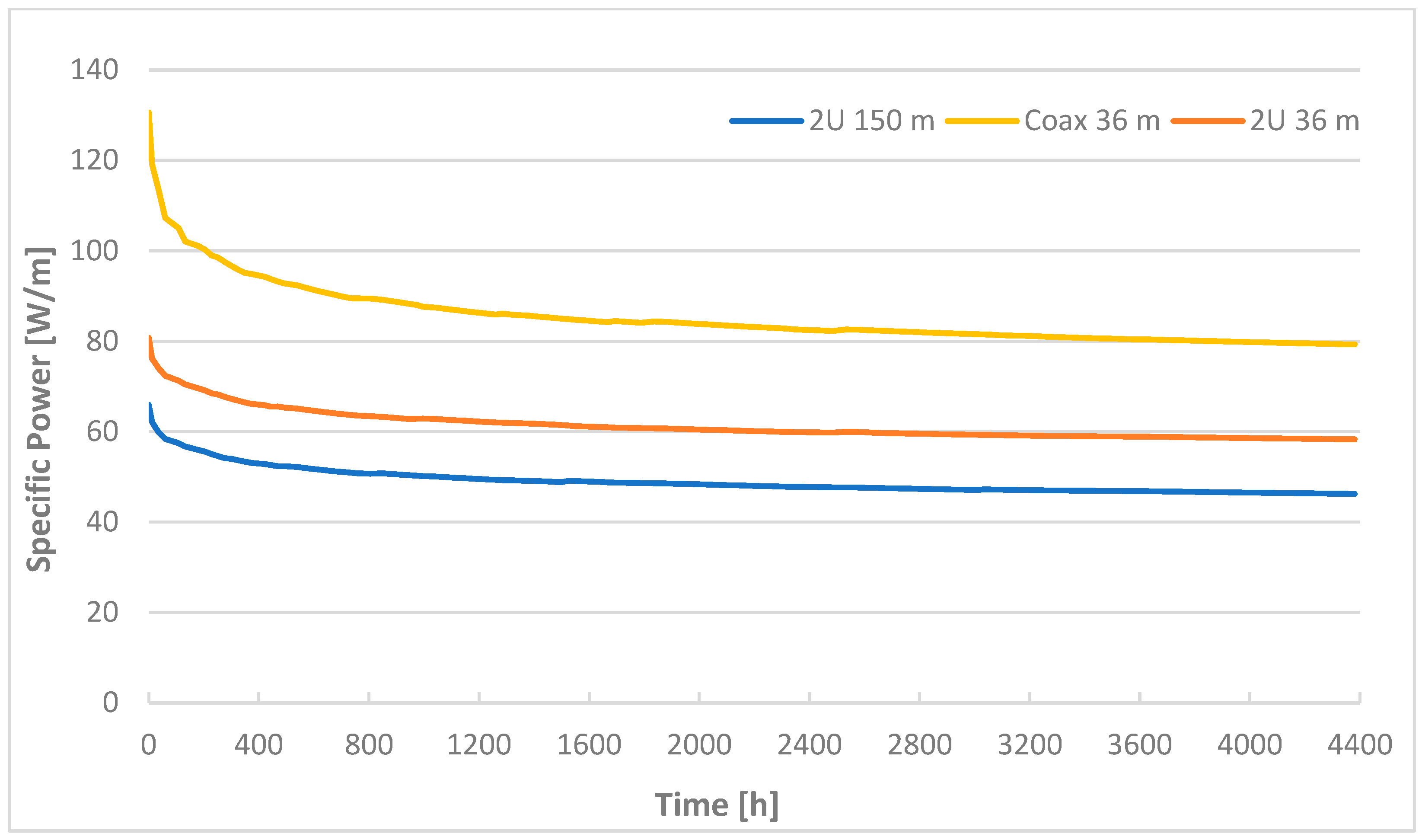
• With the same BHE geometry and material, the 2U 36 m BHE allowed for better linear thermal power extraction (56.03 W/m) compared to the 2U 150 m, which recorded a value of 42.47 W/m.
• Using the coaxial steel geometry (Coax 36 m), the linear thermal power that can be extracted increases to 74.51 W/m.
• The specific thermal power at the end of the first six months of simulation shows very similar values (2U 150 m = 46.24 W/m; 2U 36 m = 58.29 W/m; Coax 36 m = 79.32 W/m) to those recorded at the end of the five years of system operation (2U 150 m = 42.46 W/m; 2U 36 m = 55.51 W/m; Coax 36 m = 74.51 W/m). Therefore, thermal specific power decreases quite slowly after the first six months (about 5% for all the BHEs), then shows a thermal stabilization in the next few months; these results thus confirm how these data can also be used to describe the thermal performance of each BHE in long-term analysis.

Moreover, the borehole thermal resistance, which represents the temperature difference between the fluid in the BHE and the borehole wall in contact with the subsurface, shows that the coaxial pipe has the lowest value (0.020 m K W⁻¹), thus recording a significant difference compared to the double U configurations (Table 4; Figure 7).

On the other hand, the average borehole thermal resistance of the 2U BHE at −36 and −150 m depth does not show any significant difference, displaying 0.085 m K W⁻¹ and 0.081 m K W⁻¹, respectively. Calculations reported in Table 4 refer to step 5172 h, revealing only 6% difference to the final steps depicted in Figure 6.

5. Discussion

The evaluation of the thermal performance of different BHE configurations is of paramount importance in defining the specific thermal power that can be extracted and, thus, the overall thermal efficiency of a shallow geothermal system. Boreholes can indeed be equipped with different geothermal pipe geometries which can give different thermal performances. The study demonstrate that quite different energies could be extracted from the same geological framework with different BHE technologies and geometries.

The numerical simulations conducted over five years operation with three different BHE configurations revealed important insights:

• Knowledge of the right geological, hydrogeological, and thermo-physical properties of the ground is of paramount importance in correctly evaluating the thermal efficiency of BHEs.
• The specific thermal power of each BHEs records similar values to those displayed at the end of the five-year simulation already starting from the fifth month, ensuring the long-term stability of the system.
• Maintaining the same geometry and material (double U pipes in polyethylene), the pipe at −36 m showed a higher specific thermal power than that at −150 m. This confirms how at −36 m the same BHE configuration fully exploits the only aquifer present in the subsurface; as shown in Figure 4, the most favourable thermal conditions indeed occur between −9 and −36 m where the hydrodynamic characteristics of the groundwater can significantly increase the thermal efficiency. This helps in understanding how the 2U 36m BHE can be the best solution than the deeper one with the same geometry, strongly reducing drilling costs.
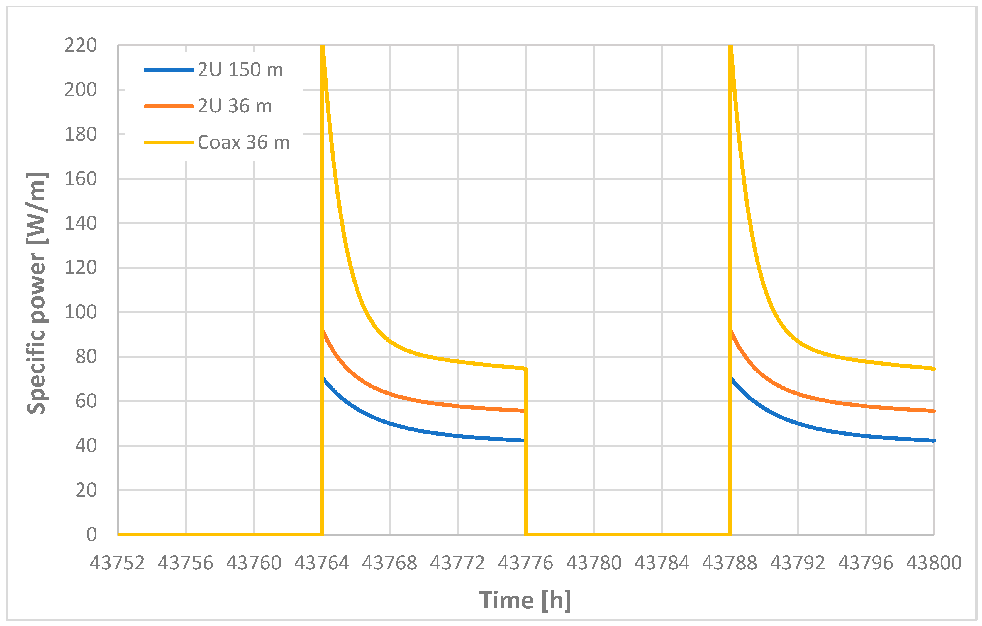
• The higher specific power of 80 [W/m] for the coaxial configuration differs from values found in the literature for which the highest value recorded is equal to 42.2 W/m [46], which is, however, based only on the thermo-technical characteristics of the BHE without considering the hydrogeological and geological parameters that can potentially contribute to the heat power also exceeding 80 W/m in some scenarios.
• The coaxial geometry proved to be not only the most efficient among the scenarios in terms of thermal power extracted but also the most thermally stable, as evidenced during intermittent operating modes with daily-on and -off cycles (12 h each); it was also easier to install on site.

The coaxial configuration also shows a lower borehole thermal resistance (0.020 m K W⁻¹, which is the best value obtained) with a relevant difference compared to the 2U geometries. The borehole thermal resistance is indeed a key performance and design parameter to evaluate. Its lowest values mean better performance but also a lower required borehole length, leading to lower total installation costs [47].

The optimization of a shallow geothermal system helps to minimize investment costs by reducing the depth and the number of drilling boreholes.

Results from numerical simulations suggest how using the coaxial design could potentially reduce the cost of drilling boreholes and make the installation easier on site, as the effective diameter would be smaller than a comparable 2U BHE. These observations are in line with previous studies [13,14,15,17,18,19,20] which highlight that the coaxial configuration outperforms the 2U BHE, and how the benefits gained in using the coaxial geometry could result in a 50% reduction in length compared to 2U, even if it might involve, at the same time, higher costs because of the stainless steel of the outer pipe instead of the most popular polyethylene type [48]. In addition, comparing the same BHE configurations (2U BHE) this study confirms how the groundwater flow can significantly improve the heat exchange rate and thus the specific thermal power, which strongly depends on the groundwater level, its flow rate and direction, and on the aquifer thickness [48]. In this regard, the better performance of the 2U 36m compared to the 2U 150 m can also be explained by a greater heat dissipation on increasing the borehole depth, leading to higher specific thermal power for shallower BHEs, which is also in line with findings by [49].

6. Conclusions

Three different borehole heat exchanger (BHE) configurations have been compared in the framework of a study aimed at integrating geothermal energy for space heating and cooling of buildings in a small city in Piedmont (NW Italy). The study confirms how a good knowledge of the underground parameters and of the aquifer characteristics are essential in the design of the BHE, providing the possibility to obtain a greater thermal specific power, by optimizing the depth and then decreasing drilling costs. This allows understanding how the hydrodynamic characteristics of the groundwater are fundamental in increasing the thermal performance of the boreholes, highlighting that the boreholes at shallow depths are thermally more efficient than the deeper ones in which poor hydrodynamic groundwater conditions occur. This confirmed the importance of doing a very detailed study of the subsoil.

Taking into account the impact that these technical features could have on the thermal efficiency of a shallow geothermal system, the main findings of this work can be summarized as follows:

• Geological, hydro-geological, and thermo-physical models should be validated through a back-analysis of the ground response test, especially for medium-large systems.
• Numerical simulations help in selecting the best heat exchanger geometry, based not only on the design or on the duty cycle but also on the thermal efficiency of the ground in terms of the amount of heat which can be extracted from it.
• Where there are lithologies with an overall thermal conductivity from medium to high, steel coaxial pipes usually perform better than conventional double U BHEs.
• The coaxial configuration outperforms the double U pipes, especially during intermittent operation modes.
• Using the coaxial loop design could potentially reduce the cost of drilling boreholes and make the installation easier on site, as the effective diameter would be smaller than a comparable double U BHE.

Using of the coaxial BHEs seems to better satisfy the required energy needs than the traditional double U. Even if more BHEs are needed, ground properties of the investigated area also allow for a simple direct push of the outer steel pipe of the coaxial BHE, saving on both the drilling and the grouting costs.

References

1. Sgaravatti, G.; Tagliapietra, S.; Trasi, C.; Zachmann, G. National Fiscal Policy Responses to the Energy Crisis. Bruegel Datasets 2023. Available online: https://www.bruegel.org/dataset/national-policies-shield-consumers-rising-energy-prices (accessed on 18 March 2025).
2. Lee, H.; Calvin, K.; Dasgupta, D.; Krinner, G.; Mukherji, A.; Thorne, P.; Trisos, C.; Romero, J.; Aldunce, P.; Barrett, K.; et al. Climate Change 2023: Synthesis Report. Sixth Assessment Report of the Intergovernmental Panel on Climate Change; Lee, H., Romero, J., Eds.; IPCC: Geneva, Switzerland, 2023; pp. 35–115. [Google Scholar] [CrossRef]
3. Moreno, D.; Nielsen, S.; Sorknæs, P.; Lund, H.; Thellufsen, J.Z.; Mathiesen, B.V. Exploring the location and use of baseload district heating supply. What can current heat sources tell us about future opportunities? Energy 2024, 288, 129642. [Google Scholar] [CrossRef]
4. Chicco, J.M.; Antonijevic, D.; Bloemendal, M.; Cecinato, F.; Goetzl, G.; Hajto, M.; Hartog, N.; Mandrone, G.; Vacha, D.; Vardon, P.J. Improving the Efficiency of District Heating and Cooling Using a Geothermal Technology: Underground Thermal Energy Storage (UTES). In New Metropolitan Perspectives NMP 2022; Lecture Notes in Networks and Systems; Calabrò, F., Della Spina, L., Piñeira Mantiñán, M.J., Eds.; Springer: Cham, Switzerland, 2022; Volume 482. [Google Scholar] [CrossRef]
5. Kavvadias, K.; Jiménez-Navarro, J.P.; Thomassen, G. Decarbonising the EU Heating Sector—Integration of the Power and Heating Sector; EUR 29772 EN; JRC114758; Publications Office of the European Union: Luxembourg, 2019. [Google Scholar] [CrossRef]
6. Goetzl, G.; Chicco, J.; Schifflechner, C.; Figueira, J.; Tsironis, G.; Zajacs, A. Pathways to better integrate geothermal energy at its full technological scale in European heating and cooling networks. Eur. Geol. 2022, 1–7. [Google Scholar] [CrossRef]
7. Boesten, S.; Ivens, W.I.; Dekker, S.C.; Eijdems, H. 5th generation district heating and cooling systems as a solution for renewable urban thermal energy supply. Adv. Geosci. 2019, 49, 129–136. [Google Scholar] [CrossRef]
8. Dumas, P. Policy and Regulatory Aspects of Geothermal Energy: A European Perspective. In Geothermal Energy and Society; Lecture Notes in Energy; Manzella, A., Allansdottir, A., Pellizzone, A., Eds.; Springer: Cham, Switzerland, 2019; Volume 67. [Google Scholar] [CrossRef]
9. Tsagarakis, K.P.; Efthymiou, L.; Michopoulos, A.; Mavragani, A.; Anđelković, A.S.; Antolini, F.; Bacic, M.; Bajare, D.; Baralis, M.; Bogusz, W.; et al. A review of the legal framework in shallow geothermal energy in selected European countries: Need for guidelines. Renew. Energy 2020, 147, 2556–2571. [Google Scholar] [CrossRef]
10. Kupfernagel, J.H.; Hesse, J.C.; Schedel, M.; Welsch, B.; Anbergen, H.; Müller, L.; Sass, I. Impact of operational temperature changes and freeze–thaw cycles on the hydraulic conductivity of borehole heat exchangers. Geotherm. Energy 2021, 9, 24. [Google Scholar] [CrossRef] [PubMed]
11. Walch, A.; Mohajeri, N.; Gudmundsson, A.; Scartezzini, J.-L. Quantifying the technical geothermal potential from shallow borehole heat exchangers at regional scale. Renew. Energy 2021, 165, 369–380. [Google Scholar] [CrossRef]
12. Casasso, A.; Sethi, R. Efficiency of closed loop geothermal heat pumps: A sensitivity analysis. Renew. Energy 2014, 62, 737–746. [Google Scholar] [CrossRef]
13. Brown, C.S.; Kolo, I.; Banks, D.; Falcone, G. Comparison of the thermal and hydraulic performance of single U-tube, double U-tube and coaxial medium to deep borehole heat exchangers. Geothermics 2024, 117, 102888. [Google Scholar] [CrossRef]
14. Quaggiotto, D.; Zarrella, A.; Emmi, G.; De Carli, M.; Pockelé, L.; Vercruysse, J.; Psyk, M.; Righini, D.; Galgaro, A.; Mendrinos, D.; et al. Simulation-Based Comparison Between the Thermal Behavior of Coaxial and Double U-Tube Borehole Heat Exchangers. Energies 2019, 12, 2321. [Google Scholar] [CrossRef]
15. Morchio, S.; Fossa, M.; Beier, R.A. Study on the best heat transfer rate in thermal response test experiments with coaxial and U-pipe borehole heat exchangers. Appl. Therm. Eng. 2022, 200, 117621. [Google Scholar] [CrossRef]
16. Bidarmaghz, A.; Narsilio, G.; Johnston, I. Numerical Modelling of Ground Heat Exchangers with Different Ground Loop Configurations for direct Geothermal Applications. In Proceedings of the 18th International Conference on Soil Mechanics and Geotechnical Engineering, Paris, France, 2–6 September 2013; pp. 3343–3346. [Google Scholar]
17. Zarrella, A.; Scarpa, M.; Carli, M.D. Short time-step performances of coaxial and double U-tube borehole heat exchangers: Modeling and measurements. HVAC&R Res. 2011, 17, 959–976. [Google Scholar] [CrossRef]
18. Harris, B.; Lightstone, M.F.; Reitsma, S.; Cotton, J.S. A numerical study on the intermittent operation of u-tube and coaxial borehole heat exchangers. Geothermics 2024, 121, 103030. [Google Scholar] [CrossRef]
19. Wood, C.J.; Liu, H.; Riffat, S.B. Comparative performance of ‘U-tube’ and ‘coaxial’ loop designs for use with a ground source heat pump. Appl. Therm. Eng. 2012, 37, 190–195. [Google Scholar] [CrossRef]
20. Wang, J. Comparative heat transfer efficiency study of coaxial and U-loop boreholes. GSTF J. Eng. Technol. 2014, 2, 1–6. [Google Scholar] [CrossRef]
21. Liu, Q.; Weiland, F.; Pärisch, P.; Kracht, N.; Huang, M.; Ptak, T. Influence of site characteristics on the performance of shallow borehole heat exchanger arrays: A sensitivity analysis. Geothermics 2023, 114, 102785. [Google Scholar] [CrossRef]
22. Schelenz, S.; Vienken, T.; Shao, H.; Firmbach, L.; Dietrich, P. On the importance of a coordinated site characterization for the sustainable intensive thermal use of the shallow subsurface in urban areas: A case study. Environ. Earth Sci. 2017, 76, 73. [Google Scholar] [CrossRef]
23. Rossi, M.; Craig, J. A new perspective on sequence stratigraphy of syn-orogenic basins: Insights from the Tertiary Piedmont Basin (Italy) and implications for play concepts and reservoir heterogeneity. Geol. Soc. Lond. Spec. Publ. 2016, 436, 93–133. [Google Scholar] [CrossRef]
24. Bertotti, G.; Mosca, P.; Juez, J.; Polino, R.; Dunai, T. Oligocene to Present kilometres scale subsidence and exhumation of the Ligurian Alps and the Tertiary Piedmont Basin (NW Italy) revealed by apatite (U-Th)/He thermochronology: Correlation with regional tectonics. Terra Nova 2006, 18, 18–25. [Google Scholar] [CrossRef]
25. Federico, C.; Pizzino, L.; De Gregorio, S.; Favara, R.; Galli, G.; Giudice, G.; Gurrieri, S.; Quattrocchi, F.; Voltattorni, N. Inverse and forward modelling of groundwater circulation in a seismically active area (Monferrato, Piedmont, NW Italy): Insights into stress-induced variation in water chemistry. Chem. Geol. 2008, 248, 14–39. [Google Scholar] [CrossRef]
26. Giraudi, C. Quaternary evolution of the plain between Casale Monferrato and Valenza: Implications for the tectonics of the Monferrato thrust front (Piedmont, NW Italy). Alp. Mediterr. Quat. 2015, 28, 71–92. [Google Scholar]
27. D’Atri, A.; Irace, A.; Piana, F.; Tallone, S.; Varrone, D.; Bellino, D.; Fioraso, G.; Cadoppi, P.; Fusetti, E.; Morelli, M.; et al. Note Illustrative Della Carta Geologica d’Italia Alla Scala 1: 50.000, Foglio 194 Acqui Terme; Istituto Superiore per la Protezione e la Ricerca Ambientale (ISPRA): Rome, Italy, 2014; pp. 1–229. [Google Scholar]
28. Quattrocchi, F.; Favara, R.; Capasso, G.; Pizzino, L.; Bencini, R.; Cinti, D.; Galli, G.; Grassa, F.; Francofonte, S.; Volpicielli, G. Thermal anomalies and fluid geochemistry framework in occurrence of the 2000–2011 Nizza Monferrato seismic sequence (northern Italy): Episodic changes in the fault zone heat flow or chemical mixing phenomena? Nat. Hazards Earth Syst. Sci. 2003, 3, 269–277. [Google Scholar] [CrossRef]
29. D’Atri, A.; Irace, A.; Piana, F.; Tallone, S.; Varrone, D.; Bellino, D.; Fioraso, G.; Cadoppi, P.; Fusetti, E.; Morelli, M.; et al. Carta Geologica d’Italia Alla Scala 1: 50.000, Foglio 194 Acqui Terme; Istituto Superiore per la Protezione e la Ricerca Ambientale (ISPRA): Rome, Italy, 2014. [Google Scholar]
30. Ghielmi, M.; Rogledi, S.; Vigna, B.; Violanti, D. La successione messiniana e plio-pleistocenica del Bacino di Savigliano (settore occidentale del Bacino Terziario Piemontese). Geol. Insubrica 2019, 13, 3–141. [Google Scholar]
31. Carrier, W.D. Goodbye, Hazen; Hello, Kozeny-Carman. J. Geotech. Geoenviron. 2003, 129, 1054–1056. [Google Scholar] [CrossRef]
32. Slater, L. Near surface electrical characterization of hydraulic conductivity: From petrophysical properties to aquifer geometries—A review. Surv. Geophys. 2007, 28, 169–197. [Google Scholar] [CrossRef]
33. Hoffmann, R.; Dietrich, P. Geoelectrical measurements for the determination of groundwater flow directions and velocities. Grundwasser 2007, 9, 194–203. [Google Scholar] [CrossRef]
34. Bibby, H.M.; Dawson, G.B.; Rayner, H.H.; Bennie, S.L.; Bromley, C.J. Electrical resistivity and magnetic investigations of the geothermal systems in the Rotorua area, New Zealand. Geothermics 1992, 21, 43–64. [Google Scholar] [CrossRef]
35. Arato, A.; Boaga, J.; Comina, C.; De Seta, M.; Di Sipio, E.; Galgaro, A.; Giordano, N.; Mandrone, G. Geophysical monitoring for shallow geothermal applications—Two Italian case histories. First Break 2015, 33, 75–79. [Google Scholar] [CrossRef]
36. Giordano, N.; Chicco, J.; Mandrone, G.; Verdoya, M.; Wheeler, W.H. Comparing transient and steady-state methods for the thermal conductivity characterization of a borehole heat exchanger field in Bergen, Norway. Environ. Earth Sci. 2019, 78, 460. [Google Scholar] [CrossRef]
37. Chicco, J.M.; Fonte, L.; Mandrone, G.; Tartaglino, A.; Vacha, D. Hybrid (Gas and Geothermal) Greenhouse Simulations Aimed at Optimizing Investment and Operative Costs: A Case Study in NW Italy. Energies 2023, 16, 3931. [Google Scholar] [CrossRef]
38. Chicco, J.M.; Mandrone, G. Modelling the energy production of a borehole thermal energy storage (BTES) system. Energies 2022, 15, 9587. [Google Scholar] [CrossRef]
39. Eklöf, C.; Gehlin, S. Ted-a Mobile Equipment for Thermal Response Test: Testing and Evaluation. Master’s Thesis, Luleå University of Technology, Luleå, Sweden, 1996; pp. 11–62. Available online: http://www.divaportal.org/smash/get/diva2:1032479/FULLTEXT01.pdf (accessed on 18 March 2025).
40. Chicco, J.M.; Mandrone, G. How a sensitive analysis on the coupling geology and borehole heat exchangers characteristics can improve efficiency and production of shallow geothermal system. Heliyon 2022, 8, e9545. [Google Scholar] [CrossRef] [PubMed]
41. Al-Khoury, P.G.; Bonnier, R. Efficient finite element formulation for geothermal heating systems. Part II: Transient. Int. J. Numer. Methods Eng. 2006, 67, 725–745. [Google Scholar] [CrossRef]
42. Diersch, H.-J.G. FEFLOW–Finite Element Modeling of Flow, Mass and Heat Transport in Porous and Fractured Media. Earth Environ. Sci. 2014, 1, 1–996. [Google Scholar]
43. Claesson, J.; Eskilsson, P. Conductive Heat Extraction by a Deep Borehole; Analytical Studies Thermal Analysis of Heat Extraction Boreholes; Department of Mathematical Physics, University of Lund: Lund, Sweden, 1987; pp. 1–26. [Google Scholar]
44. Gehlin, S.; Bo, N. Determining undisturbed ground temperature for thermal response test. ASHRAE Trans. 2003, 109, 151–156. [Google Scholar]
45. Chicco, J.M.; Verdoya, M.; Giuli, G.; Invernizzi, C. Thermophysical properties and mineralogical composition of the Umbria-Marche carbonate Succession (Central Italy). In The Geological Society of America. Special Paper. 250 Million Years of Earth History in Central Italy: Celebrating 25 Years of the Geological Observatory of Coldigioco; Koeberl, C., Bice, D.M., Eds.; The Geological Society of America: Boulder, CO, USA, 2019; p. 542. [Google Scholar] [CrossRef]
46. He, X.; Li, J.; Chen, Y.; Niu, B. Analysis on heat transfer performance of coaxial borehole heat exchanger in a layered subsurface with groundwater. Heliyon 2024, 10, e37442. [Google Scholar] [CrossRef] [PubMed]
47. Javed, S.; Spitler, J. Accuracy of borehole thermal resistance calculation methods for grouted single U-tube ground heat exchangers. Appl. Energy 2017, 187, 790–806. [Google Scholar] [CrossRef]
48. Jia, G.S.; Ma, Z.D.; Xia, Z.H.; Wang, J.W.; Zhang, Y.P.; Jin, L.W. Influence of groundwater flow on the ground heat exchanger performance and ground temperature distributions: A comprehensive review of analytical, numerical and experimental studies. Geothermics 2022, 100, 102342. [Google Scholar] [CrossRef]
49. Chen, J.; Qiao, W.; Xue, Q.; Zheng, H.; An, E. Research on ground-coupled heat exchangers. Int. J. Low-Carbon Technol. 2010, 5, 35–41. [Google Scholar] [CrossRef]
Figure 2. ERT results: (a) electrical resistivity, (b) chargeability, and (c) geological conceptual model. In both (a,b), the main geological layers and formations are depicted as in the geological interpretation provided in (c). In (c), colours of the geological layers correspond to the same colours as in Figure 1, except for the landfill in the first meters.
Smartcities 08 00121 g002
Figure 3. Inlet (red), outlet (blue), and average (green) temperature recordings from the field TRT (continuous lines) vs. those simulated numerically (dashed lines). Simulated average temperature is given with a 2% confidence interval.
Smartcities 08 00121 g003
Figure 4. Final thermogeological model of the investigated area. Kxx, Kyy, and Kzz represent the hydraulic conductivity along the X, Y, and Z directions; λs is the thermal conductivity of the solid; ϕ is the porosity; and T is the undisturbed ground temperature.
Smartcities 08 00121 g004
Figure 5. Comparison between specific power extraction (W/m) at the 12th hour of each on-cycle (12 h cycle on and 12 h cycle off), which can be extracted from the three different geothermal BHE configurations, during the first six months of the five-year simulation corresponding to the time slot between 0 and 4380 h.
Smartcities 08 00121 g005
Figure 6. Comparison between specific power extraction (W/m) which can be extracted from the three different geothermal BHE configurations, during the last 48 h of the five-year simulation corresponding to the time slot between 43,752 and 43,800.
Smartcities 08 00121 g006
Figure 7. Comparison of the borehole thermal resistance (Rb, m K W−1) for the three different BHE geometries.
Smartcities 08 00121 g007