Improving Time Series Data Quality: Identifying Outliers and Handling Missing Values in a Multilocation Gas and Weather Dataset

Highlights

What are the main findings?

• A hybrid rule-based and statistical method significantly improves detection of outliers in time series gas and weather data across multiple locations.
• An imputation strategy combining temporal and spatial information leads to more reliable handling of missing values.

What is the implication of the main finding?

• The proposed methods enhance the quality of environmental sensor data to be used in descriptive and predictive analytics.
• This approach can be adapted to other domains with similar challenges in multivariate time series datasets.

Abstract

High-quality data are foundational to reliable environmental monitoring and urban planning in smart cities, yet challenges like missing values and outliers in air pollution and meteorological time series data are critical barriers. This study developed and validated a dual-phase framework to improve data quality using a 60-month gas and weather dataset from Jubail Industrial City, Saudi Arabia, an industrial region. First, outliers were identified via statistical methods like Interquartile Range and Z-Score. Machine learning algorithms like Isolation Forest and Local Outlier Factor were also used, chosen for their robustness to non-normal data distributions, significantly improving subsequent imputation accuracy. Second, missing values in both single and sequential gaps were imputed using linear interpolation, Piecewise Cubic Hermite Interpolating Polynomial (PCHIP), and Akima interpolation. Linear interpolation excelled for short gaps (R² up to 0.97), and PCHIP and Akima minimized errors in sequential gaps (R² up to 0.95, lowest MSE). By aligning methods with gap characteristics, the framework handles real-world data complexities, significantly improving time series consistency and reliability. This work demonstrates a significant improvement in data reliability, offering a replicable model for smart cities worldwide.

1. Introduction

Handling outliers and missing values is a critical challenge in data management. This challenge is especially significant for time series data, as its sequential nature introduces complexities not found in static datasets lacking temporal dependencies. In conventional datasets, outliers are often identified using standard statistical techniques, and missing values are managed through methods like mean or median imputation [1,2]. However, these traditional approaches fail to account for the temporal dependencies inherent in time series data, treating each data point independently [3]. This oversight can lead to significant inaccuracies, as the continuity, trends, and patterns within the data are essential for meaningful analysis. For example, in environmental datasets, failing to consider these temporal structures can distort analyses and lead to flawed predictions, ultimately affecting decision-making processes [4].

Time series data present unique challenges, such as autocorrelation, where each observation is influenced by preceding values, and seasonality, which introduces repeating patterns over time [3]. These factors complicate the application of traditional methods. Anomalies like outliers can disrupt these patterns, skewing analytical models and reducing their predictive accuracy [5,6]. Similarly, missing data points, often caused by sensor malfunctions, transmission issues, or environmental factors, disrupt the sequence of observations and risk losing critical temporal patterns [7]. Addressing these challenges requires advanced methods that not only clean the dataset but also preserve its temporal and structural integrity.

In smart cities, where decision-making relies heavily on accurate, real time data, addressing these data imperfections is especially critical [8]. Decision makers, urban planners, environmental analysts, and policymakers depend on high-quality datasets to monitor air quality, design mitigation strategies, and evaluate public health interventions [9,10]. For example, erroneous or missing air pollution data can lead to misleading insights, impacting the effectiveness of regulatory measures and the allocation of resources. The increasing adoption of Internet of Things (IoT) sensors in smart cities has further highlighted the importance of robust data-management strategies, as these sensors often generate vast amounts of time series data that are prone to inconsistencies and gaps [11,12]. Improving data quality is therefore foundational for effective urban management, supporting the creation of smarter, more sustainable cities.

This study employs the need for advanced outlier-identification methods that preserve temporal structure and minimize information loss [5]. Outlier detection serves as the necessary first step in improving data quality, as undetected anomalies can skew imputation methods, leading to biased or inaccurate results [6]. For instance, gas-concentration readings outside plausible environmental ranges often indicate issues. These can include sensor errors, data-transmission failures, or readings below detection limits [3]. These zero readings present a unique challenge, as their nature cannot always be determined due to a lack of supporting metadata. Consequently, in this study, zero values were treated as outliers and flagged for removal to avoid potential biases in subsequent analyses.

By addressing these issues first and treating outliers as missing values, the framework ensures a cleaner, more reliable dataset. This preprocessing step significantly enhances the effectiveness of imputation techniques, ensuring that temporal structure and data integrity are maintained [13]. Such an approach is particularly critical in time series datasets, where preserving continuity and avoiding distortions is essential for accurate downstream analyses and decision-making.

Missing values in time series data require specialized imputation techniques that consider both the continuity and variability of the data. The goal is not merely to fill gaps but to restore missing data in a way that reflects realistic trends and preserves the dataset’s temporal coherence [13,14]. Advanced methods, including machine learning-based techniques such as K-Nearest Neighbors (KNN) or LSTM Bayesian neural network with nonparametric dynamic thresholding (ConvLSTMBNN-DT), offer promising solutions for handling these challenges [7]. By combining these methods with statistical techniques, we aim to build a robust framework for addressing data quality issues in environmental datasets [4].

This research focuses on gas concentrations and meteorological data collected from ten monitoring stations in Jubail Industrial City, Saudi Arabia, over 60 months. These datasets, which are integral to smart city systems, present unique challenges due to their size, complexity, and susceptibility to errors and gaps. By addressing these challenges, the study provides practical tools and methodological advancements for improving data quality in time series datasets. Our approach combines statistical methods, such as Interquartile Range (IQR) and Z-Score, with machine learning-based techniques, including Local Outlier Factor (LOF) and Isolation Forest, to identify and handle outliers while preserving the dataset’s temporal integrity. Missing values are then addressed using a combination of interpolation, regression-based, and machine learning-based imputation methods, tailored to the dataset’s specific characteristics.

The main contributions of this study are as follows: (1) We develop a dual-phase data quality pipeline for environmental time series, combining statistical and machine learning techniques for outlier detection and imputation. (2) We propose a sequential strategy for handling zero values, isolated gaps, and prolonged missing sequences that preserves temporal integrity. (3) We apply curvature-aware interpolation methods, specifically PCHIP and Akima. These methods preserve the natural shape of time series data during imputation. They significantly reduce error, with MSE between 0.002 and 0.004, and R² values between 0.95 and 0.97, on a 14-million-record dataset from the Royal Commission. (4) We demonstrate that the proposed workflow is adaptable to other smart city and IoT datasets with minimal adjustments. To guide this work, we address the following research questions:

Research Question 1: How can data-management strategies improve the quality of the data on urban planning and environmental monitoring in smart cities?

This question highlights the foundational role of data management in ensuring accurate and reliable datasets, which are essential for effective decision-making in urban planning and environmental monitoring.

Research Question 2: What methods can be most effective for handling missing values in time series data, and how will these methods influence the reliability and accuracy of environmental condition assessments in smart cities?

This question focuses on identifying the most effective techniques for imputation and interpolation, evaluating their impact on the reliability of environmental assessments critical for urban management.

These contributions strengthen the broader field of smart city analytics and environmental monitoring. The proposed methods help ensure that data-driven insights more accurately reflect real-world conditions by minimizing the impact of outliers and missing values. By improving data quality at the source, this work supports more resilient, data-informed decision-making for sustainable urban development and public health planning.

This paper is organized as follows: Section 2 (Previous Work), reviews related work. Section 3 (Data Description), we describe the dataset used for this study, including its structure, sources, and key characteristics, setting the stage for the subsequent analysis. Section 4 (Methodology) outlines the methods employed for outlier detection, handling missing values, and improving data quality. In Section 5 (Results), we present the outcomes of applying the proposed methodologies, highlighting the effectiveness of the approaches and discussing their impact on data quality. Section 6 (Discussion) provides an in depth interpretation of the results, critically evaluating the methodologies and their implications for future studies. Finally, Section 7 (Conclusions) summarizes the key findings of this work, discusses its contributions, and suggests potential directions for future research.

2. Previous Work

Maintaining high data quality is crucial for time series datasets, particularly in applications such as environmental monitoring and smart city systems [15,16]. Time series data often suffer from imperfections, including outliers, missing values, and inconsistencies introduced by IoT-generated data [15]. These issues can significantly impact the reliability of predictive models and decision-making processes [16]. Over the years, researchers have developed various approaches to address these challenges, ranging from statistical methods to advanced machine learning models [16]. This section reviews the key contributions in the field, focusing on outlier detection, missing value imputation, and the specific challenges posed by IoT-based environmental data. By identifying the limitations of existing methods, this review establishes the foundation for developing a framework to improve data quality in time series datasets.

Conventional statistical methods, such as Z-Score and the IQR, are commonly used for outlier detection. Akouemo and Povinelli [17] provide an extensive review of statistical outlier-detection methods in time series data. While effective, these methods often fail to account for temporal dependencies, leading to potential misclassifications in time series datasets. Appaia and Palraj [18] emphasize the importance of domain-specific thresholds for identifying outliers in environmental datasets. For instance, zero readings for gas concentrations are physically implausible under normal conditions and are treated as outliers. Incorporating such domain knowledge ensures that detected anomalies reflect real world constraints. Sharma and Singh [19] further highlight how domain-specific knowledge can enhance the accuracy of anomaly detection in smart city applications. However, these methods often overlook the integration of domain knowledge with temporal dependencies, which this research seeks to address.

Machine learning models, including supervised and unsupervised approaches, have been extensively used for outlier detection. Li et al. [20] discuss the integration of domain knowledge into anomaly-detection algorithms, enhancing their accuracy in identifying contextually relevant anomalies. Bansal et al. [21] highlight the use of clustering-based and deep learning models for identifying outliers in complex datasets. Recent studies, such as Zhu et al. [22] and Fang et al. [23], explore ensemble methods and hybrid models that leverage multiple algorithms to improve the robustness of anomaly detection. ARIMAX models have also been applied to extract time series characteristics and identify outliers through residual hypothesis testing, demonstrating robustness in maintaining temporal consistency [17]. While these models improve detection capabilities, there is still a lack of unified frameworks that effectively incorporate both machine learning models and domain-specific thresholds for complex environmental datasets.

Time series-specific imputation methods, such as Seasonal Decomposition and Exponential Smoothing State Space Models, focus on preserving temporal patterns. Hyndman and Athanasopoulos [3] describe these approaches in the context of forecasting, demonstrating their utility in maintaining seasonal and trend components during imputation. Bansal et al. [21] extend this by incorporating hybrid approaches that combine statistical and machine learning models to improve accuracy in environmental datasets where seasonality and autocorrelation are prominent. In addition, Sharma and Singh [19] categorize imputation techniques into statistical, machine learning, and hybrid methods, highlighting the trade offs between simplicity, computational efficiency, and accuracy. Although these methods have shown promise, challenges remain in handling prolonged missing intervals and leveraging inter-variable relationships, particularly in multi-sensor datasets.

Prolonged missing intervals and cases where relationships between variables can be leveraged have motivated the application of regression-based techniques. These models ensure that the imputed values align with the observed patterns in the dataset. Similarly, Zhang and Zhou [14] discuss combinatorial deep neural model for missing values imputation in air quality, particularly effective when addressing gaps in sensors with block missing and long-interval consecutive missing and does not require repeated modeling. Despite these advancements, regression-based techniques often lack scalability for large-scale, real-time applications, which are critical for smart city systems.

Machine learning techniques, such as K-Nearest Neighbors (KNN), have been widely adopted for missing value imputation due to their ability to account for complex nonlinear relationships. Jadhav and Kulkarni [24] provide a state of the art review of these techniques, emphasizing their robustness in high-dimensional datasets. Advanced methods, including neural network-based imputations, have also been explored to capture intricate temporal dependencies. Zainuddin et al [13] discuss how neural networks enhance the accuracy of imputations by leveraging temporal structures in the data. Additionally, Jin et al. [25] highlight the potential of deep learning models in handling large-scale time series data with missing values. The integration of neural networks into imputation workflows is in line with the growing need for scalable and accurate solutions. However, the challenge of balancing computational efficiency and accuracy remains.

The increasing adoption of IoT sensors in smart cities has underscored the need for robust data-management strategies. Gilman et al. [26] and Syed et al. [8] discuss challenges related to inconsistencies and gaps in IoT-generated time series data. These works emphasize the importance of leveraging inter-sensor relationships and advanced imputation techniques to address missing values and improve data quality. Sharma and Singh [19] further elaborate on the role of IoT-based data analytics in improving urban decision-making and sustainability. Multi-source approaches that extract patterns across datasets have also proven effective in improving the reliability of environmental datasets [20].

High-quality datasets are essential for environmental monitoring. Bibri and Krogstie [9] explore air quality monitoring in smart cities, emphasizing the role of accurate data in regulatory measures and public health interventions. Tsokov et al. [4] discuss hybrid spatiotemporal models for air pollution forecasting, combining CNN and LSTM to handle large-scale environmental datasets. Shekhar et al. [27] advance this further by focusing on spatiotemporal data-mining methods to uncover hidden patterns in environmental data, enhancing the applicability of these models to addressing real world challenges. Benchmark datasets such as Weather2K [22] provide opportunities to evaluate forecasting models under real-world conditions, which directly informs validation processes for imputation and outlier detection.

Recent advances highlight the role of deep learning and probabilistic methods in handling missing values. DeepMVI [21] showcases the robustness of neural networks in capturing complex dependencies in time series data. Bayesian models, such as BayOTIDE [23], add value by handling irregular sampling and quantifying uncertainty, providing confidence intervals for critical imputations to applications such as air quality monitoring. Practical tools like the “imputeTS” package [28] further emphasize the need for accessible workflows for preprocessing time series data.

Previous research on missing data in environmental sensor networks has largely focused on imputation techniques [29,30,31]. Although valuable, these techniques often operate under assumptions that may not hold in real world scenarios, particularly when dealing with complex datasets containing various types of missingness such as zero values, single missing values, and sequences of missing values. Zero values represent instances where sensors report no concentration of a substance, which may be due to actual absence, sensor malfunction, or values below the detection limit. Single missing values are isolated instances where a sensor fails to report a reading, often surrounded by valid data points. Sequences of missing values involve consecutive missing readings, indicating prolonged sensor issues or data-transmission failures. Furthermore, broader data quality frameworks, such as those discussed in Practical Data Quality [32], tend to concentrate on data governance and organizational aspects. They tend not to focus on the technical details of missing data handling for error minimization. This research directly addresses this gap by developing a methodology (Section 4) that prioritizes the sequential handling of different types of missing value to minimize the introduction of errors before any imputation or analysis is conducted. This approach is crucial because the treatment of one type of missingness can significantly affect the treatment of others.

These studies collectively emphasize the importance of leveraging domain-specific knowledge, advanced statistical methods, and machine learning approaches to preserve temporal and spatial dependencies. Despite significant progress, challenges remain to integrate these methods into a unified framework to address data imperfections in time series datasets. Current approaches often fail to fully capture the interplay between outlier detection, imputation methods, and spatiotemporal dependencies, particularly in the context of environmental datasets with IoT-generated data. Building on these foundations, our research aims to develop a robust and systematic framework to improve data quality. This framework integrates spatiotemporal data mining [27], domain knowledge [18], and addresses specific IoT-driven challenges [26]. The goal is to ensure the reliability of the data used in smart city and environmental monitoring systems. By addressing these limitations, this work seeks to uncover new insights and provide practical tools that improve decision-making processes and policy interventions through accurate and scalable solutions.

Recent studies have applied deep learning models to impute missing values in time series data. These include Transformer-based models for EEG signal restoration [33], 1D-CNNs for atmospheric data filtering [34], and LSTM-based autoencoders for long-term gap imputation in environmental datasets [35,36]. These methods have demonstrated strong capabilities in modeling nonlinear temporal dependencies, especially in high-resolution or multivariate contexts. However, their complexity, data requirements, and tuning overhead make them less practical for many real-time or resource-constrained applications.

3. Data Description

Environmental monitoring in smart cities requires high-resolution, accurate data to assess air quality and weather patterns. This study utilizes a unique dataset collected from Jubail Industrial City, Saudi Arabia, which provides insights into the challenges and opportunities of handling time series data in complex urban environments. With hourly gas and weather measurements from ten monitoring locations, this dataset supports the development of robust data-management strategies to improve data quality for urban planning and environmental monitoring.

3.1. Dataset Overview

The dataset includes hourly measurements of both gas pollutants and meteorological variables, covering a period of 60 months from January 2018 to December 2022. Jubail Industrial City, with its blend of industrial and residential zones, serves as an ideal case study for environmental monitoring (see Figure 1). The gas data in

Table 1. Gas pollutant variables for all 10 sensors from (January 2018–December 2022).

Gases Categorized by Pollutants Units	Unit	Collected
CO, H2S	parts per million (ppm)	Hourly
SO2, NO, NO2, NOx, NH3, NMHC, THC, Benzene, Ethyl Benzene, (m,p-xylene), o-Xylene, Toluene	parts per billion (ppb)	Hourly

include pollutants such as carbon monoxide (CO), hydrogen sulfide (H₂S), sulfur dioxide (SO₂), nitric oxide (NO), nitrogen dioxide (NO₂), oxides of nitrogen (NO_x), ammonia (NH₃), and non-methane hydrocarbons (NMHC). Advanced metrics, such as NMHC 3-h rolling average, total hydrocarbons (THC), benzene, ethyl benzene, MP-xylene (m,p-xylene), o-xylene, and toluene, are also captured.

Meteorological data in

Table 2. Meteorological variables for all 10 sensors from (January 2018–December 2022).

Category	Variables	Unit	Collected
Air Temperature	2 m, 10 m	°C	Hourly
Soil Temperature	−0.05 m, −1.0 m, −2.0 m	°C	Hourly
Relative Humidity	NA	%	Hourly
Atmospheric Pressure	NA	hPa	Hourly
Solar Radiation	NA	W m−2	Hourly
Wind (10 m, 50 m, 90 m)	Speed, Direction	m s−1, °	Hourly

encompass atmospheric temperature (at 2 m and 10 m heights), relative humidity (RH), pressure (PRES), and solar radiation (SR). Wind speed and direction are recorded at 10 m, 50 m, and 90 m, while soil temperature is monitored at depths of −0.05 m, −1.0 m, and −2.0 m below ground level. This extensive dataset provides valuable insights into both short term fluctuations and long term trends.

3.2. Focus on Carbon Monoxide (CO)

While data for multiple pollutants are available, this study primarily focuses on carbon monoxide (CO) as a representative pollutant. CO was selected due to its relevance in urban air quality studies and its association with vehicular and industrial emissions. Moreover, the challenges presented by CO data, such as outliers and missing values, make it an ideal candidate for demonstrating the effectiveness of the proposed data-management framework. The methodology developed here can be extended to other pollutants in future analyses.

3.3. Data Organization and Storage

The dataset is organized by sensor and year, with each file containing hourly measurements. Each file follows a consistent naming convention (S1_2018.***) for streamlined analysis. Although no official metadata were provided, we created a custom data dictionary to document variable names, units, and data-processing steps. This organization ensures efficient analysis and supports reproducibility, providing a transparent framework for handling large-scale environmental datasets.

3.4. Data Quality Considerations

Maintaining data quality is essential for meaningful analysis. Gas concentrations should never be zero or negative; such values indicate potential sensor errors or transmission issues and are treated as outliers. Similarly, sudden spikes in gas concentrations, often caused by sensor anomalies or unusual environmental events, disrupt typical data patterns and require careful handling. These data quality issues directly impact the imputation process and subsequent analyses. The methods used to address these challenges are detailed in the methodology section.

3.5. Spatial Context

The sensor network in Jubail Industrial City spans both residential and industrial zones. Each zone has distinct environmental characteristics, which adds complexity to the dataset. For example, industrial areas may experience more emissions, while residential zones are influenced by different microclimates. These location-specific factors directly affect gas concentrations and weather patterns. Figure 1 shows where sensors are placed, with industrial zones marked in red and residential zones in blue. To improve data quality, we adjusted preprocessing steps to reflect these geographical differences. This helped address challenges such as sensor bias and uneven spatial coverage. We also considered localized effects, such as industrial heat islands, when building statistical models. These adjustments helped ensure more accurate analysis of urban conditions, including how pollution spreads across the city.

By addressing the dataset’s unique challenges, including spatial variability, temporal gaps, and data anomalies, the preprocessing phase established a robust foundation for subsequent outlier detection and missing value imputation. The following sections detail the methods and techniques applied to ensure data integrity and analytical reliability.

4. Methodology

To operationalize the proposed framework, we designed a structured data quality pipeline tailored for environmental time series. The approach combines domain-aware statistical analysis with machine learning techniques to detect and correct anomalies, preserving temporal continuity and minimizing imputation error.

This study implements a thorough data-processing methodology to ensure the accuracy and reliability of gas (specifically CO) and weather data analysis in Jubail Industrial City. Raw data obtained from environmental sensors are often compromised by anomalies, outliers, and missing values, which can negatively impact the validity of subsequent analyses. The methodology, illustrated in Figure 2, comprises three interconnected stages: data preprocessing, outlier handling, and missing value imputation. Throughout each stage, quality control is maintained through a combination of visual inspection of time series plots and statistical checks to prevent data distortion.

The initial preprocessing stage focuses on two key areas. First, all received files are standardized into a consistent CSV format to ensure uniformity and seamless integration of data from multiple sources. Second, we addressed the erroneous zero values present in the CO sensor data. Given the environmental context, it is physically implausible for CO concentrations to reach zero. Therefore, these values are identified as artifacts, removed from the dataset, and replaced with NaN (Not a Number) to distinguish them from valid measurements. Following zero removal, single missing values (isolated NaN values) are identified and handled using linear interpolation. This method estimates the missing value by drawing a straight line between the two neighboring known values, which preserves the continuity of the time series and prepares the dataset for accurate outlier detection.

The next stage involves outlier detection and handling. Several outlier-detection methods were evaluated, including IQR, Z-score, and Local Outlier Factor (LOF). Ultimately, the Isolation Forest (IsoForest) algorithm was selected due to it is superior performance in identifying anomalous data points. The IsoForest algorithm identifies outliers based on their isolation in the feature space, points that are easily isolated are considered outliers. Identified outliers are temporarily removed from the dataset to prevent them from unduly influencing the subsequent missing value-imputation process.

The core of the methodology lies in the imputation of missing values. To thoroughly evaluate various imputation techniques, 10% of the data points were randomly selected and artificially set to NaN. This created a controlled benchmark for comparing the imputed values with known true values. The remaining missing values (both original and artificially induced) were classified as either single missing values or sequential missing values (consecutive NaN values). The single missing values were interpolated using linear interpolation, as described in the preprocessing step. For sequential missing values, a range of imputation techniques were carefully tested, including linear interpolation, spline interpolation, k-Nearest Neighbors (k-NN) imputation, and Multivariate Imputation by Chained Equations (MICE). The optimal imputation method for sequential missing values was determined through comparative analysis. The performance of all imputation methods (both single and sequential) was evaluated using multiple metrics, including the coefficient of determination (R²), Mean Squared Error (MSE), and Mean Absolute Error (MAE). The primary objective was to maximize R² while minimizing both MSE and MAE.

Finally, after the optimal imputation techniques were identified and applied, the temporarily removed outliers were reintroduced into the dataset, specifically those outliers with very high values observed only rarely within the five-year data range. This critical step ensures that the final processed dataset retains all original data points, including those representing genuine extreme events, thus preserving the inherent variability of the environmental data and providing a complete and accurate dataset for subsequent analysis. Therefore, the complete methodology ensures that all original data are used in the analysis, with only the non-valid data receiving specialized treatment.

Throughout the entire process, quality-control measures are implemented to validate each step. These measures ensure that preprocessing maintains data consistency, outlier detection identifies only true anomalies, and imputation methods align with the expected characteristics of the data. Each step in this methodology is carefully designed to minimize inconsistencies and prepare the dataset for a better future environmental analysis.

4.1. Data Preprocessing

The data-preprocessing phase involved several critical steps to ensure that the dataset was clean, consistent, and ready for imputation and further analysis. All preprocessing tasks were performed using Python 3.9, leveraging powerful libraries such as Pandas 2.2 [37], NumPy 1.24 [38], the built-in Datetime module (Python 3.9) [39] for data manipulation, PyJanitor 0.23 [40], and Matplotlib 3.6 [41] for visual validation of data consistency.

The first step involved standardizing all received files into a consistent CSV format to ensure uniformity and enable seamless integration. Using Python’s file-handling capabilities, data from multiple sources were merged into a single dataset. Any unstructured or semi-structured data were transformed into a tabular format using Pandas, ensuring all variables were organized as columns and observations as rows. The duplicate records were then identified and removed to eliminate redundancy. We dropped irrelevant columns that were not required for imputation or further analysis to simplify the dataset. Units of measurement were standardized across variables to address inconsistencies between sensors. For example, gas concentrations were converted to parts per million (ppm), and temperatures were unified in degrees Celsius. These conversions were performed using NumPy for efficient mathematical operations. Subsequently, we aligned timestamps with a uniform hourly frequency to maintain temporal consistency. Missing timestamps were identified and inserted as placeholders for later imputation. The datetime module was used to handle time alignment and ensure that all records adhered to a consistent time format. Data types were verified and corrected to ensure that the numeric values, categorical variables, and timestamps were appropriately formatted, avoiding issues during later analytical stages. Finally, metadata such as sensor locations were integrated into the dataset wherever available. These metadata were essential to provide context and improve the interpretability of the data. Throughout this phase, Matplotlib was used to visually inspect data trends and verify the success of the preprocessing steps. For example, time series plots were generated to check for gaps and unexpected problems in the data. These preprocessing steps were carefully designed to handle the diverse challenges presented by the raw data, ensuring that the dataset was clean, structured, and ready for subsequent phases of outlier detection and missing value handling.

4.2. Handling Zero Values

The datasets present several challenges, including zero values, single missing values, and sequences of missing values. These will be addressed sequentially, with the order of operations being crucial because handling one type of missingness can impact how subsequent types are addressed (see Figure 3), which illustrates the different types of missing values and the distribution of zeros across all sensors. This section focuses on the first issue: zero values. In environmental sensor data, zero values can represent true measurements (zero precipitation), values below the detection limit, or sensor malfunctions. Ideally, these scenarios would be treated differently. However, due to the complexity of the dataset and the lack of complete sensor specifications and error mode information, a conservative approach is adopted. All zero values are considered missing values (NaN). This prevents erroneous assumptions and ensures that they do not unduly influence the interpolation of adjacent missing data or subsequent analyses.

4.3. Identifying and Addressing Single Missing Values

Ensuring data quality is paramount in datasets with temporal dependencies, such as environmental sensor data. Missing values disrupt the continuity of the data, leading to potentially misleading analyses and inaccurate predictions. For example, a gap in gas-concentration measurements (ozone or particulate matter) during a pollution event could delay public health warnings, while missing meteorological data (temperature or wind speed) during extreme weather might prevent accurate modeling of storm impacts or heatwave risks. Among these issues, missing values situated between two known values are particularly critical, as they introduce inconsistencies that can compromise the integrity of temporal trends and the reliability of downstream analyses to reflect actual conditions. This study outlines a robust methodology for handling these missing values, involving three key stages: identifying missing values between two known values, interpolating them using a linear interpolation approach, and validating the results by comparing interpolated values to expected trends and examining residuals. This methodology not only restores data continuity but also aligns interpolated values with the context provided by surrounding data points. For longer sequences of missing data, multiple imputation techniques were tested; these are evaluated in subsequent sections.

4.3.1. Identifying Single Missing Values

The first step involves identifying single missing values that occur between two known values in the same sensor time series. To ensure chronological consistency, the dataset is first sorted by time index. We then create a boolean mask using pandas.isnull() to flag all missing values. This mask is a sequence of True (for missing) and False (for present) values (see Figure 3).

We define three intermediate masks:

• mask_na = s.isnull()                     marks missing entries.
• prev_ok = s.shift(1).notna()    marks entries whose predecessor is non-missing.
• next_ok = s.shift(-1).notna()      marks entries whose successor is non-missing.

We then compute

$$\mathtt{single}\_\mathtt{gap}=\mathtt{mask}\_\mathtt{na}\&\mathtt{prev}\_\mathtt{ok}\&\mathtt{next}\_\mathtt{ok},$$

which flags exactly those NaN positions flanked by valid entries on both sides. For example, in the sequence [10, NaN, 30], the missing value at index 1 is correctly detected. More importantly, the algorithm also handles patterns like [10, NaN, 5, NaN, 5], where multiple isolated NaNs appear. Each NaN is flanked by valid values and is therefore identified as a single missing value. This method explicitly excludes consecutive or boundary NaNs, which fail at least one neighbor check. Those cases are handled separately using forward-fill and backward-fill to maintain continuity when interpolation is not feasible. The entire process is implemented in Python using Pandas and NumPy, and results are visually verified by overlaying the detection mask on the raw time series.

4.3.2. Interpolating Missing Values Using Linear Interpolation

Once the missing values have been identified, the next step involves filling them using linear interpolation. As described in Section 4.2, zero values will be considered missing and filled using linear interpolation (see Figure 4, which shows a heatmap to the single missing values was successfully interpolated. Linear interpolation is well-suited for this task as it assumes a linear trend between the two known values surrounding the missing entry, which, while not always perfectly accurate, is often a reasonable approximation for environmental variables over the hourly intervals used in this dataset. Other more sophisticated methods were evaluated, but were deemed computationally intensive.

4.3.3. Validation and Rechecking

To validate the interpolation process and ensure the integrity of the dataset, a multifaceted approach is employed. First, the resulting interpolated values are checked to ensure they remain within the range defined by their neighboring known values. This step prevents the introduction of unrealistic or spurious values that could arise from extrapolation (predicting values outside the range of known data). After this initial check, the dataset is rechecked for any remaining missing values using the same boolean masking technique described in Section 4.3. This confirms that all identified missing values, including those initially recorded as zero (as mentioned in Section 4.2), between two known values have been successfully filled. A heatmap is generated to visualize any remaining missing values, providing a clear and intuitive view of the completeness of the dataset after interpolation. Furthermore, key statistical summaries, such as the mean, standard deviation, median, and select percentiles (25th, 75th), are calculated for each sensor’s data both before and after the interpolation process. The percentage change in each statistic is calculated and required to be within a margin of 5%, a value chosen to balance the need for data fidelity with the inherent uncertainty of interpolation. This comparison ensures that the interpolation process has not unduly altered the overall distribution and statistical properties of the data, thus confirming that the adjustments align with the overall characteristics and trends of the dataset.

4.4. Outlier Detection

Outlier detection was a critical step in ensuring the integrity of the dataset, focusing on identifying and addressing both unexpected high values and unexpected low values, such as zeros. This process aimed to prevent extreme or anomalous data points from distorting subsequent analyses, particularly during the imputation of missing values. A combination of statistical methods (IQR, Z-Score), machine learning-based techniques (LOF, Isolation Forest), and domain-specific considerations was used to identify and address outliers effectively. Importantly, the definitions of outliers and errors were tailored to this specific dataset, recognizing that these thresholds may vary between different datasets and contexts.

In our dataset, spanning five years of continuous monitoring, the highest recorded CO concentration was 8 parts per million (ppm), occurring only once. Given the rarity of this value, we have established 8 ppm as the upper threshold for valid CO measurements, since the maximum values that CO reach in 5 years is less than 8. Consequently, any readings exceeding this limit are classified as errors, as they are considered physically implausible within the environmental context of our study. These anomalous data points are probably due to sensor malfunctions or data-transmission issues. To preserve the integrity and consistency of our dataset, these erroneous values are flagged and addressed appropriately, which may involve removal, imputation, or separate analysis, depending on the nature and extent of the anomaly.

In contrast, sudden increases in CO concentrations from typical patterns are identified as outliers. Although these spikes might represent genuine environmental fluctuations, they are marked for further scrutiny as a result of their departure from established trends. It is important to note that CO levels up to 8 ppm are considered valid within our processed dataset, this value serves as the maximum acceptable limit, not as an error threshold.

This approach aligns with established air quality standards. The National Ambient Air Quality Standards (NAAQS) set by the Environmental Protection Agency (EPA) designate 9 ppm as the maximum allowable concentration (the safe range level) over an eight hour average [42]. By setting our threshold at 8 ppm, we ensure that our data remains within recognized safe exposure levels, thereby enhancing the reliability of our findings.

Supporting this threshold, a study by Javors et al. [43] examined breath carbon monoxide levels and found that a cut off level of 8 ppm or higher is often used to identify smoking status. This suggests that CO concentrations at or above this level are indicative of CO exposure (Low level concern), reinforcing our decision to classify readings beyond 8 ppm as errors in our environmental dataset.

To identify outliers, statistical techniques such as the IQR method and Z-Score analysis were applied [1,2]. The IQR is defined as $Q_3-Q_1$, where $Q_1$ and $Q_3$ are the 25th and 75th percentiles of the data. A reading is flagged as an outlier if it lies below $Q_1-1.5\times \mathrm{IQR}$ or above $Q_3+1.5\times \mathrm{IQR}$. For example, for CO at sensor S1 we have $Q_1=0.282$ ppm and $Q_3=0.617$ ppm, so $\mathrm{IQR}=0.335$ ppm. This gives thresholds of $0.282-1.5\times 0.335\approx -0.225$ ppm (truncated to 0 ppm) and $0.617+1.5\times 0.335=1.1195$ ppm; any CO value outside [0, 1.1195] ppm is therefore flagged as an outlier. Similarly, the Z-Score method identified data points with values greater than 3 or less than −3 as potential outliers [3]. Recognizing the temporal structure of the data, these methods were adjusted using rolling window statistics, calculating Z-Scores and IQR values within a moving window to account for local trends and seasonal patterns [13]. We used a rolling window of 7 days, corresponding to short-term local trends without smoothing out valid anomalies. This adjustment ensured that normal temporal fluctuations were not mistakenly classified as outliers.

Machine learning-based methods, including Local Outlier Factor (LOF) and Isolation Forest, were also employed to enhance the detection process. Isolation Forest complemented these methods by isolating anomalous data points through random decision trees, efficiently detecting global and local outliers in complex datasets [5]. For Local Outlier Factor (LOF), we used n_neighbors = 20 to ensure sensitivity to local fluctuations while minimizing false positives in dense regions. Isolation Forest was configured with n_estimators = 1000 and contamination = 0.02, reflecting the low expected frequency of anomalies. These settings were chosen based on empirical tuning and alignment with prior studies in environmental monitoring

Domain-specific thresholds played a crucial role in refining the detection process. For example, while CO values above 8 ppm were flagged as errors specific to this dataset, the definition of outliers was based on the patterns and normal ranges observed in this particular dataset. These thresholds were dataset-specific and may differ in other studies or contexts. Zero values, which are physically implausible for gas concentrations, were also flagged as anomalies because gas concentrations cannot drop to zero under normal conditions [6].

Once identified, outliers and errors were treated in the same manner as missing values to maintain consistency in the data quality-improvement process. These values were replaced using imputation techniques such as interpolation, k-Nearest Neighbors imputation, or time series specific models, depending on the context. Visual validation was performed to ensure that the treated values integrated smoothly with the dataset. Time series plots were generated to inspect the corrected values, confirming that they aligned with the overall trends and patterns observed in the data and that no artificial jumps or discontinuities were introduced.

This tailored approach to outlier detection emphasized the importance of dataset specific thresholds and the need to differentiate between errors and outliers. By adequately addressing both types of anomalies, this methodology safeguarded the integrity and reliability of the dataset for subsequent analysis.

4.5. Handling Missing Values

Handling missing values was a critical step in ensuring the completeness, reliability, and usability of the dataset for time series analysis, especially given its importance for downstream tasks such as predictive modeling and accurate trend identification. Missing data in the dataset resulted from various causes, including sensor malfunctions, communication errors during data transmission, and deliberate removal of values flagged as errors or outliers during preprocessing (as described in Section 4.4). These missing values were not uniformly distributed, with some sensors exhibiting short single gaps, while others experienced extended periods of missing data, particularly at the boundaries of the dataset. This variability in missing data posed a significant challenge and required the application of a combination of statistical, regression-based, machine learning-based, and time series specific methods to ensure that the imputation process was accurate and consistent with the temporal structure of the dataset [14].

We implemented the imputation process in Python, leveraging libraries such as Pandas for data manipulation [44], NumPy for efficient numerical operations [45], scikit learn for machine learning-based methods [46], and statsmodels for time series specific techniques such as Kalman Smoothing [47]. This ensured computational efficiency and reproducibility throughout the process. The first step involved a detailed analysis of the patterns and distribution of missing values between sensors and time intervals, which helped guide the selection of appropriate imputation methods [13].

For short single gaps, simple interpolation methods such as linear interpolation were applied due to their ability to provide quick and reliable estimates of smooth trends in the data [48]. For scenarios requiring smoother transitions, cubic spline interpolation was used, which ensures that the overall shape of the data remains intact [49]. Piecewise Cubic Hermite Interpolation Polynomial (PCHIP) was employed for more complex scenarios, as it preserves monotonicity and smoothness over larger gaps [50]. Kalman Smoothing was prioritized for noisy datasets with sequence gaps, providing temporally consistent estimates by smoothing out variations [51].

For sequence missing intervals (consecutive missing values) or cases where relationships between variables could be leveraged, regression-based techniques were applied. Multiple linear regression models were used to predict missing values based on other correlated variables, such as weather conditions or gas concentrations from neighboring sensors [13]. These methods were particularly effective when addressing gaps in sensors with strong inter-variable dependencies, ensuring that imputed values aligned with observed patterns in the dataset.

Advanced machine learning-based imputation methods were used to handle intricate patterns of missingness. The K-Nearest Neighbors (KNN) algorithm, using a defined time window to select neighbors, estimated missing values by analyzing the similarity of neighboring observations, effectively capturing localized patterns in the data [13]. Transferred Multiple LSTM based deep auto-encoder (TMLSTM-AE), which uses spatial and time series information to fill in single missing, multiple missing, block missing, and long-interval consecutive missing in air quality data looking for more accurate and consistent predictions [14].

4.6. Validate the Handling Missing Values

To validate the effectiveness of the imputation methods, a carefully designed evaluation framework was implemented. A subset of the original dataset (10% of existing values, a proportion commonly used in imputation validation studies) was intentionally removed, simulating missing data, and imputation methods were applied to estimate these values. The imputed results were then compared with the original data to assess the accuracy of each method using metrics such as MSE and MAE. Sensitivity analysis was conducted by introducing small random perturbations (adding Gaussian noise with a standard deviation of 1% of the data range) to the imputed dataset and evaluating the stability of key statistical summaries and trend analyses, ensuring that the imputation process preserved critical patterns and relationships in the data. Visual validation, including time series plots generated using Matplotlib, confirmed that the imputed values aligned seamlessly with the observed trends, ensuring consistency across all sensors. This multifaceted approach addressed the challenges posed by the variability and complexity of missing data in time series datasets. By employing a diverse range of techniques and leveraging domain knowledge, the methodology ensured that the imputed dataset retained its temporal coherence, cross-sensor relationships, and overall integrity. This process not only enhanced the quality of the dataset but also established a reliable foundation for subsequent analyses, such as environmental trend identification and predictive modeling. As demonstrated in the results section, the chosen methods effectively minimized imputation errors, contributing to the robustness of the study’s findings.

4.7. Quality-Control Measures

To ensure the accuracy, reliability, and consistency of the dataset, quality-control measures were implemented at every stage of the workflow, spanning preprocessing, outlier detection, and handling missing values. These measures were designed to reduce errors, maintain data integrity, and validate the effectiveness of the applied methods. The approach adhered to best practices established by the Open Geospatial Consortium (OGC) Sensor Web Enablement (SWE) standard [52] and methodologies for air quality monitoring systems [53,54].

During preprocessing, we standardized the raw data files into a uniform format to address structural inconsistencies caused by variations across sensors. Gas concentrations were expressed in parts per million (ppm), temperatures were converted to degrees Celsius, and wind speeds were standardized to meters per second. Timestamps were aligned according to the ISO 8601 [55] format to ensure temporal coherence. Consistency checks included verifying that numerical fields contained valid values and confirming the adherence of column names to a unified schema. Error logging using Python’s logging module captured discrepancies such as missing files, invalid entries, or structural mismatches. Additionally, random samples of the cleaned data were manually inspected to validate transformations, ensuring that gas concentration ranges and timestamp alignments conformed to predefined standards.

Quality checks during outlier detection focused on validating flagged anomalies to ensure that only genuine outliers were addressed. time series plots were generated using Matplotlib to visually inspect anomalies and confirm deviations from expected trends. For domain-specific thresholds, such as CO levels exceeding 8 ppm, flagged values were reviewed against known physical limits and sensor operational conditions. This step was critical in distinguishing between sensor errors and plausible environmental anomalies. Furthermore, cross-sensor comparisons were conducted for measurements taken at the same location to assess inter-sensor reliability [54].

Handling missing values required robust validation measures to ensure the reliability of the imputation process. Artificial gaps were introduced into the dataset, and metrics such as MSE and MAE were calculated to assess performance, while sensitivity analysis was performed by perturbing the imputed data with random noise to evaluate the robustness of the imputation process. Visual inspections of time series plots ensured that imputed values integrated seamlessly with the overall trends and patterns in the dataset. Statistical checks, including recalculating descriptive metrics such as means, medians, and variances, confirmed that the imputed dataset preserved the original structure and variability.

Post-processing involved additional quality-control steps to ensure that the dataset maintained its structural integrity and temporal coherence. Automated rule-based checks were implemented to continuously monitor data quality. For instance, predefined limits, such as CO levels that do not exceeding 8 ppm, triggered alerts for manual review. Anomaly detection using recalculated Z-Scores identified any remaining outliers, with values exceeding ±3 flagged for further investigation. These steps ensured that the dataset adhered to physical constraints and industry standards [56].

The final validation focused on verifying the completeness and consistency of the dataset after all quality-control measures were applied. Summary statistics, including means, medians, and standard deviations, were recalculated for each variable and visualized using boxplots and histograms to inspect any changes in the data distribution. Temporal coherence was validated by examining time series plots for irregularities such as unexplained jumps or gaps. Missing timestamps were flagged and addressed through interpolation, ensuring continuity in the temporal structure of the data [3]. Cross-sensor comparisons were reviewed to confirm that relationships between variables were preserved, further improving the reliability of the dataset.

By integrating these quality-control measures throughout preprocessing, outlier detection, and missing value imputation, the methodology ensured the dataset’s structural integrity, and temporal coherence. Validation processes, including statistical checks, visual inspections, and sensitivity analyses, provided confidence in the reliability of the dataset for predictive modeling and environmental trend analysis. These measures established a robust framework for handling large-scale, complex time series datasets in environmental monitoring.

5. Results

5.1. Impact of Preprocessing

The preprocessing phase successfully transformed the raw, unstructured data into a clean and consistent dataset suitable for time series analysis. A total of thirty raw data files were standardized into a consistent CSV format and merged into a single dataset containing more than 14.5 million data values within 30 columns, approximately 483,120 rows. This dataset represents gas and weather data collected from ten locations over 60 months. During the data-cleaning process, we identified and removed duplicate records, which reduced the dataset by 2.8%. These steps streamlined the dataset and improved its manageability, ensuring a cleaner and more reliable foundation for analysis.

To address inconsistencies between variables, the units of measurement were standardized, ensuring uniformity across all sensors. For example, gas concentrations were converted to parts per million (ppm), and temperatures were standardized to degrees Celsius. Standardizing units eliminated discrepancies between sensors and allowed accurate cross-sensor comparisons, crucial for detecting trends and relationships in environmental monitoring. The timestamps were aligned with a uniform hourly frequency, ensuring temporal consistency throughout the dataset (see Figure 5). This alignment process revealed 217 missing timestamps, representing less than 0.01% of the total expected timestamps, which were inserted as placeholders to maintain the integrity of the time series data for later imputation. In addition, metadata, such as sensor locations, was integrated where available, providing essential contextual information for spatial analyses and enhancing the interpretability of environmental trends across the monitored locations.

Throughout the preprocessing phase, visual validation using Matplotlib revealed significant improvements in data consistency. Time series plots confirmed the elimination of anomalies caused by inconsistent units and duplicate records, while the temporal alignment of the data was verified. These preprocessing efforts significantly enhanced the accuracy and reliability of the dataset, ensuring that it could effectively support environmental monitoring and urban planning analyses in smart city systems, such as air quality forecasting and pollution source identification. This strong foundation facilitated subsequent steps, including outlier detection and the handling of missing values.

5.2. Identifying and Addressing Missing Values Between Two Known Values

The results of this methodology demonstrate clear and measurable improvements in data quality. In all cases, the number of missing values between two known values was reduced to zero. Linear interpolation effectively restored data continuity, ensuring that the interpolated values aligned with the contextual trends of the flanking values. The application of interpolation also enhanced the coherence of temporal patterns, as confirmed through statistical validation and visualization. Statistical summaries (including mean, variance, and median, as shown in

Table 3. The difference during the interpolation process to the mean and variance of the dataset, which remained consistent.

Sensors	Mean	Variance	Median
S1	0.07%	0.08%	0.00%
S2	0.06%	0.08%	0.00%
S3	0.01%	0.05%	0.00%
S4	0.12%	0.07%	0.20%
S6	0.05%	0.16%	0.00%
S8	0.06%	0.12%	0.18%
S9	0.06%	0.01%	0.00%
S10	0.09%	0.03%	0.23%
S11	0.02%	0.15%	0.24%
S12	0.04%	0.17%	0.00%

) revealed that the dataset remained statistically consistent before and after the interpolation process, confirming that the method preserved the dataset’s inherent structure. This aligns with the validation criteria, where the expected percentage change must be less than 5%. The visualization of the heatmap provided a clear representation of the success, with no missing values remaining between two known values visible in the final dataset (see Figure 4).

5.3. Outlier Detection

Outlier detection effectively identified and addressed errors and anomalies in the dataset, ensuring data quality and consistency for subsequent analyses. For CO, values exceeding 8 parts per million (ppm) were classified as errors, reflecting implausible measurements likely caused by sensor malfunctions or data-transmission issues. No CO readings above this threshold were found in the dataset. Similarly, zero values across all gas measurements, which are physically implausible, were identified as an error. Approximately 0.9% of the total gas concentration readings were flagged as zero values, representing a significant portion of the non realistic measurements.

In addition to errors, sudden spikes in CO values were identified as outliers, Figure 6 shows that clearly, as they represented abrupt deviations from the normal data range and patterns. These spikes accounted for 0.1% of the flagged CO data points and were identified using both statistical methods and machine learning-based techniques. Statistical methods such as the Z-Score and IQR approach successfully flagged extreme values, while rolling window statistics adjusted for local trends and seasonal patterns, ensuring that regular temporal fluctuations were not misclassified as outliers. Machine learning techniques, including Local Outlier Factor (LOF) and Isolation Forest, identified localized anomalies, particularly in areas with varying data densities. Together, these methods provided a robust mechanism for detecting anomalies in the dataset. By combining statistical and machine learning approaches, the outlier-detection process ensured that anomalies were accurately identified across different data patterns.

Following identification, the flagged errors and outliers were treated as missing values (see

Table 4. CO distribution across sensors. The green areas represent the ranges where most of the data points are concentrated; as the frequency of data points increases, the green hue becomes darker, indicating higher density. Conversely, the red areas indicate ranges with little to no data points, highlighting regions of low or zero density.

CO	S1	S2	S3	S4	S6	S8	S9	S10	S11	S12
0.1	6178	2961	4658	4001	6372	1364	6991	6471	7586	4161
0.3	13,688	9647	18,825	12,007	13,025	8842	17,760	14,598	14,278	14,796
0.5	13,994	14,296	15,267	15,283	12,724	16,763	10,733	13,082	15,760	13,222
0.7	9114	13,342	5199	10,691	11,339	12,152	6571	7528	7061	9670
0.9	2929	4963	1345	3775	3037	4600	3698	3741	1914	3800
1.1	644	1162	897	808	396	1374	948	724	199	880
1.3	96	258	237	158	91	533	221	258	48	231
1.5	40	48	54	39	4	230	34	170	36	66
1.7	14	18	17	18	2	138	15	84	11	22
1.9	7	13	6	9	0	75	6	86	4	9
2.1	3	9	9	0	0	42	2	2	0	2
2.3	1	4	7	1	0	29	5	4	1	1
2.5	2	3	5	0	1	9	3	3	0	0
2.7	3	3	4	0	0	8	1	5	0	1
2.9	0	0	0	1	0	2	3	0	1	0
3.1	0	4	2	0	0	0	1	0	0	0
3.3	0	0	1	0	0	1	1	1	0	0
3.5	0	0	1	0	1	0	0	0	2	1
3.7	0	0	0	0	0	0	2	1	0	0
3.9	0	2	0	0	0	0	0	0	0	0
4.1	0	2	0	0	0	0	2	0	0	0
4.3	0	0	0	0	0	0	1	0	0	0
4.5	0	1	0	0	0	2	0	2	0	0
4.7	0	0	0	0	0	0	0	2	0	0
4.9	2	0	0	0	0	0	1	1	0	0
5.1	0	0	0	0	0	1	2	0	0	0
5.3	0	0	0	0	0	0	0	0	0	0
5.5	0	0	0	1	0	0	0	0	0	0
5.7	0	0	0	0	0	0	0	0	0	0
5.9	0	0	0	0	0	0	0	0	0	0
6.1	0	0	0	0	0	0	0	0	0	0
6.3	0	0	0	0	0	0	0	0	0	0
6.5	0	0	0	0	0	0	0	0	0	2
6.7	0	0	0	0	0	0	0	0	0	2
6.9	0	0	0	1	0	0	0	0	0	0
7.1	0	0	0	0	0	0	0	0	0	0
7.3	0	0	0	0	0	0	0	0	0	0
7.5	0	0	0	0	0	0	0	0	0	0
7.7	0	0	0	0	0	0	0	1	0	0

). In this table, the distribution of CO concentrations is visualized using a color gradient. The green areas represent the ranges where most of the data points are concentrated, as the frequency of data points increases, the green hue becomes darker, indicating higher density. In contrast, the red areas indicate ranges with little to no data points, highlighting regions of low or zero density. Notably, around a CO concentration of 1.2 ppm, there is a sharp decline in data density, as evidenced by the transition from green to light green and then to red. This abrupt decrease suggests that CO concentration values exceeding 1.2 ppm are infrequent and may be considered outliers. Since gases should never have a concentration of exactly zero, any such readings were flagged as outliers, in addition to other extreme values (see Figure 7 and Figure 8). Removing these outliers resulted in significant performance improvements, particularly in the PCHIP and Akima interpolation methods, where the MSE values decreased from 0.0047 to 0.0024. This reduction in MSE by almost 50% underscores the importance of addressing outliers before performing missing value imputation. This improvement satisfies the validation criteria and requires a significant decrease in MSE values after the removal of the outliers. Visual validation through plots confirmed that the identified and treated values aligned smoothly with the overall trends and patterns of the data, ensuring that the temporal integrity of the dataset was preserved.

By identifying and treating errors and anomalies, the outlier-detection process ensured that the dataset accurately reflected the level of pollution in the real world, allowing more reliable analyses for urban planning and environmental monitoring. These steps improved the reliability and usability of the dataset, laying the foundation for robust imputation methods and subsequent environmental analyses.

5.4. Effectiveness of Imputation Methods

The imputation process successfully addressed the missing values in the dataset, ensuring temporal consistency, preserving cross-sensor relationships, and improving overall data quality. Missing values were imputed using a combination of interpolation, regression-based, machine learning-based, and time series specific methods, tailored to the characteristics and distribution of the gaps. The analysis revealed that the dataset had a missing data range of approximately 1% to 4%, with most missing values resulting from sensor malfunctions or communication errors. These findings address Research Question 2 by identifying effective methods for handling missing values and demonstrating their impact on the reliability and accuracy of environmental condition assessments in smart cities.

For short single missing values between known values, interpolation techniques such as linear interpolation provided seamless transitions in the data. This method achieved high accuracy, as reflected in their low MSE as low as 0.0012 and R-squared values ranging from 0.90 to 0.97 (average of 0.94) during validation.

For sequence missing values, among these, PCHIP and Akima interpolation were particularly effective, achieving MSE values between 0.002 and 0.004 and higher R² scores (up to 0.95), making them ideal for datasets with nonlinear trends. Regression-based techniques such as multiple linear regression and stochastic regression leveraged inter-variable dependencies, providing moderate improvements, particularly for sensors with strong correlations to other variables, but with higher MSE values than interpolation methods. Machine learning-based methods, including KNN performed exceptionally well for complex patterns of missingness, particularly in datasets with nonlinear relationships. The KNN algorithm was effective in capturing localized patterns, while MICE iteratively refined imputed values, resulting in improved overall accuracy. As part of finding the best method, we even tried advanced time series specific methods such as Kalman Smoothing and Seasonal-Trend decomposition using Loess (STL) decomposition were instrumental in maintaining temporal integrity, with STL decomposition effectively handling seasonal patterns and trends. For STL decomposition, we used a seasonal window size of 13 and a trend window of 15, and enabled robust fitting to reduce sensitivity to outliers. These parameters were selected based on typical weekly and monthly seasonal cycles in the data and provided the best reconstruction fidelity in our tests.

Both regression-based imputations estimate a missing CO concentration at time t by regressing on its immediate temporal neighbors. Concretely, we fit

$${\widehat{CO}}_t={\beta }_0+{\beta }_{1}C{O}_{t-1}+{\beta }_{2}C{O}_{t+1}+{\epsilon }_t,$$

where $C{O}_{t-1}$ and $C{O}_{t+1}$ are the known CO measurements at the preceding and following time steps. For the KNN imputer, we use a univariate approach: each non-missing time point s is represented by its scalar $C{O}_s$; distances are computed as

$$d(s,t)=|C{O}_s-C{O}_t|,$$

we set $k=5$, and the imputed value is

$${\widehat{CO}}_t={\displaystyle \frac{1}{k}}\sum _{i\in N_k\left(t\right)}C{O}_i,$$

where $N_k\left(t\right)$ denotes the set of the k nearest neighbors of time t in CO space.

We recognize that using more variables such as other gases or weather data could improve accuracy. But in this study, we chose a simple approach that focuses only on CO values at $t-1$ and $t+1$. This helped reduce computational cost while keeping the method efficient. In our experiments, this univariate method performed well. It reached R² ≈ 0.94 on held-out gaps. Adding more inputs gave only small gains and did not justify the extra complexity.

Our validation process confirmed the effectiveness of the methods we applied. Artificially removed data (10% from the dataset) were successfully recovered with high accuracy. Across all methods, MSE values ranged from 0.001 to 0.005, representing less than 0.1% of the typical range of values for the measured variables. Sensitivity analysis, introducing random noise to the imputed values, confirmed the stability of the imputation process. The MSE on the original imputed data was 0.04222, while the MSE on the perturbed data was 0.04229. This represents a change of only 0.16%, indicating that the imputation methods are highly robust to small perturbations in the data (see Figure 9). Visual validation through time series plots further confirmed that the imputed values aligned seamlessly with the dataset’s overall trends and patterns (see Figure 10 and Figure 11, which clearly shows the missing values imputation area).

By employing a diverse set of imputation methods, this study ensured a reliable dataset for subsequent predictive modeling and environmental trend analysis. The findings highlight the importance of selecting appropriate techniques based on the characteristics of missing data and demonstrate how effective imputation can improve the reliability of datasets for urban planning and environmental monitoring in smart cities. A breakdown of the methods and their performance is provided in

Table 5. MSE for different imputation methods under varying outlier-handling thresholds. “Normal” indicates no outlier handling, while IQR 1.5 and IQR 3 refer to outlier-detection thresholds where data points beyond 1.5 and 3 times the IQR were removed. Using the stricter IQR 1.5 threshold is expected to yield better results by reducing extreme outliers that may negatively impact model performance.

Rank	Method	Normal	IQR 3	IQR 1.5
1	PCHIP (Best preferred)	0.00470	0.00327	0.00241
2	Akima	0.00474	0.00328	0.00242
3	Linear	0.00486	0.00337	0.00249
4	Time	0.00486	0.00337	0.00249
5	Kalman Smoothing	0.00500	0.00338	0.00250
6	Polynomial (order = 2)	0.00607	0.00376	0.00282
7	Quadratic	0.00607	0.00376	0.00282
8	Cubic	0.00650	0.00391	0.00295
9	Nearest	0.00812	0.00587	0.00446
10	KNN Imputer	0.00901	0.00683	0.00525
11	Backward Fill	0.00951	0.00674	0.00525
12	Forward Fill	0.00991	0.00711	0.00541
13	Hot Deck Imputation	0.00991	0.00711	0.00541
14	EWMA (span = 3)	0.01039	0.00779	0.00607
15	Moving Average (median (w = 3))	0.01067	0.00760	0.00584
16	Moving Average (mean (w = 3))	0.01067	0.00760	0.00584
17	EWMA (span = 5)	0.01133	0.00877	0.00687
18	EWMA (halflife = 2)	0.01167	0.00912	0.00717
19	Moving Average (mean (w = 6))	0.01413	0.01090	0.00856
20	Moving Average (median (w = 6))	0.01438	0.01168	0.00923
21	Moving Average (mean (w = 12))	0.01687	0.01387	0.01108
22	Moving Average (median (w = 12))	0.01749	0.01484	0.01194
23	STL Decomposition	0.02328	0.01979	0.01661
24	MICE Imputer	0.05000	0.04725	0.04295
25	EM Algorithm	0.05000	0.04725	0.04295
26	Iterative Imputer	0.05000	0.04725	0.04295
27	Regression Imputation	0.05002	0.04732	0.04298
28	Spline (order = 3)	0.05464	0.05096	0.04504
29	Spline (order = 2)	0.05630	0.05260	0.04649
30	Spline (order = 1)	0.05755	0.05377	0.04752
31	Mean Imputation	0.05860	0.05482	0.04856
32	Expanding Mean	0.05870	0.05482	0.04857
33	Stochastic Regression	0.05909	0.05562	0.04982
34	Median Imputation	0.05934	0.05545	0.04894
35	Mode Imputation (Least preferred)	0.24053	0.23578	0.22525

, showing the results across different outlier-handling techniques.

Key Findings

The dataset contained 0.9% zero values, randomly distributed across the gas and weather sensors. These zeros, representing a portion of a total of 3.9% missing values, posed significant challenges that required robust imputation techniques to ensure data integrity and reliability. A comparative analysis of various imputation methods was performed, and the results are summarized in Table 5. Key findings are discussed below:

• Piecewise Polynomial Interpolation (PCHIP, Akima, Cubic, Quadratic): PCHIP and Akima interpolation were the top performing methods. PCHIP achieved the lowest MSE of 0.00470, consistently delivering superior performance under all tested conditions. Its ability to preserve the data’s shape without introducing artifacts makes it the most robust choice, especially for handling non linear trends. The Akima interpolation was closely followed with an MSE of 0.00475, excelling in datasets with abrupt changes. Cubic and Quadratic interpolation, while effective, introduced slightly higher errors (MSE of 0.00650 and 0.00607, respectively) due to their tendency to overshoot.
• Linear and Similar Interpolations (Linear, Time): Linear- and time-based interpolations achieved identical MSE values of 0.00486. These methods provided a straightforward approach, performing well in datasets with predominantly linear trends, but were slightly outperformed by PCHIP and Akima.
• Kalman Smoothing: Kalman Smoothing (MSE = 0.00500) demonstrated strong performance by leveraging past and future data points. Its ability to account for temporal dependencies makes it well suited for time series data.
• K-Nearest Neighbors (KNN) Imputation: KNN imputation (MSE = 0.00901) struggled in this dataset due to its sensitivity to outliers and computational complexity.
• Exponential Weighted Moving Averages (EWMA): EWMA methods (span = 3, MSE = 0.01039; span = 5, MSE = 0.01133) effectively smoothed short-term fluctuations but struggled with long-term patterns and sudden changes, leading to higher MSEs.
• Moving Averages (Mean and Median): The 3-window Moving Average (mean) method produced an MSE of 0.01067. Increasing the window size to 12 significantly increased the error (mean MSE = 0.01688, median MSE=0.01749), indicating excessive smoothing.
• Regression and Advanced Methods: Regression Imputation (MSE = 0.05002) and higher order spline methods (order = 3, MSE = 0.05464; order = 2, MSE = 0.05631) showed significant limitations, likely due to overfitting or overshooting.
• Mode Imputation: Mode Imputation resulted in the highest MSE (0.24053), proving unsuitable for this complex, time-dependent dataset.

The analysis (summarized in Table 5) clearly demonstrates the superiority of advanced interpolation methods such as PCHIP and Akima for handling missing values in this complex environmental time series dataset. These methods outperformed simpler and more resource-intensive alternatives. Although Kalman Smoothing was effective for datasets with strong temporal dependencies, methods like EWMA and Moving Averages had limitations. The careful selection of imputation techniques, tailored to the dataset’s specific characteristics, is critical for ensuring data integrity and reliability.

5.5. Post-Preprocessing Data Validation

The post-preprocessing data validation demonstrated the effectiveness of quality-control measures to ensur the reliability, consistency, and readiness of the dataset for analysis. Structural integrity checks confirmed that all gas and weather measurements were standardized into consistent units, such as gas concentrations in parts per million (ppm), temperature in degrees Celsius, and wind speed in meters per second. Summary statistics, including mean, median, and standard deviation, were recalculated after preprocessing, confirming that the dataset remained within expected physical limits and domain specific thresholds, such as all temperature readings falling between 5 °C and 52 °C, and all gas concentrations remaining within established safety limits.

Temporal coherence was validated by inspecting time series plots, which revealed smooth trends with no unexplained gaps or abrupt jumps. Missing timestamps identified during preprocessing were successfully filled using interpolation methods, ensuring a continuous and synchronized temporal structure across all sensors. The alignment of timestamps confirmed the success of temporal standardization, with all readings accurately synchronized. Visual inspections further validated that transitions between observed and imputed values were seamless, maintaining temporal consistency without introducing artificial distortions.

Outlier-removal validation showed that flagged anomalies, such as CO readings above 8 ppm, were appropriately handled without distorting the dataset. Recalculated Z-Scores confirmed that all values fell within ±3 standard deviations of the mean, ensuring that no anomalies were overlooked.

The accuracy of the missing value-imputation process was validated by introducing artificial gaps in the dataset and comparing the imputed results with original values. The MSE for imputed values ranged from 0.001 to 0.005, demonstrating high accuracy across all variables. Sensitivity analysis, where imputed values were perturbed with random noise, showed minimal impact on key statistical summaries and subsequent analyses, with variations remaining below 0.1%. Time series plots of the imputed data revealed seamless integration of missing values, with imputed points aligning naturally with existing trends. These findings validate the accuracy and reliability of the imputation methods, addressing Research Question 2.

Cross sensor consistency was assessed after preprocessing and imputation, ensuring that relationships between variables remained intact. CO levels measured by one sensor exhibited expected correlations with weather variables, such as temperature and wind speed, recorded by nearby sensors. The average correlation coefficient between CO and temperature across sensors was 0.75, indicating a strong positive relationship. No significant discrepancies were observed between sensors measuring the same parameters, confirming the dataset’s suitability for multi-sensor and multi-variable analysis. These results directly address Research Question 1, which demonstrate how data-management strategies improved data quality for environmental monitoring and urban planning.

In summary, post-preprocessing validation confirmed that the dataset met the required standards for accuracy, completeness, and consistency. The applied quality-control measures effectively removed errors, handled missing values, and preserved both the dataset’s structural and temporal integrity. This validated dataset provides a reliable foundation for downstream tasks such as predictive modeling, environmental trend analysis, and smart city decision-making.

5.6. Impact on Subsequent Analyses

This subsection details how the completed preprocessing and quality-control steps positively influenced the reliability and accuracy of further data analysis, directly addressing research objectives. The preprocessing and quality-control measures significantly improved the accuracy and reliability of subsequent analyses. By addressing structural inconsistencies, temporal misalignments, and missing data, the cleaned and validated dataset provided a robust foundation for predictive modeling and environmental trend analysis. These results directly address Research Question 1, demonstrating how data-management strategies improved dataset quality for environmental monitoring, and Research Question 2, highlighting how effective imputation methods enhanced the reliability of trend detection and predictive modeling.

Handling outliers, such as a single large jump within a five-year period, minimized noise and distortions, ensuring that the correlation analyses between gas concentrations and weather variables reflected true environmental patterns rather than anomalies caused by sensor irregularities. Furthermore, the accurate imputation of missing values preserved the temporal coherence of the time series data, enabling robust trend detection and reducing bias in time-dependent analyses.

These preprocessing steps also enhanced the performance of analytical models, as demonstrated by lower error rates and more reliable predictions. For example, predictive models trained on the preprocessed dataset achieved a 15% reduction in MAE compared to models trained on the raw data, a substantial improvement that enhances the reliability of predictions for air quality forecasting. The seamless integration of imputed values ensured continuity across sensors, which was critical for multivariate analyses involving gas and weather variables. This consistency enabled the identification of subtle trends and patterns, supporting more informed environmental monitoring and urban planning.

Overall, the preprocessing workflow ensured that subsequent analyses were robust, reproducible, and capable of generating meaningful and actionable insights. These findings underscore the importance of high-quality data management in producing reliable results for environmental monitoring systems and smart city applications. Future work could explore the integration of automated pipelines to enhance the scalability and efficiency of these preprocessing techniques.

6. Discussion

6.1. Reflection on Preprocessing

The preprocessing phase played a critical role in ensuring the reliability and usability of the dataset. Standardizing the data across multiple sources resolved significant inconsistencies, such as variations in file formats, units of measurement, and timestamps. The use of Python’s Pandas library was instrumental in managing these challenges, particularly in handling inconsistencies in timestamp formats. Functions like pd.to_datetime() allowed for flexible and efficient standardization, while metadata gaps, such as missing sensor location details, were addressed manually using archived paper records and older digital files. While effective, this process highlighted the need for automated metadata handling to reduce the reliance on manual intervention.

Aligning timestamps to a uniform hourly frequency proved essential for maintaining the temporal integrity of the dataset. By identifying and inserting missing timestamps, representing approximately 0.4% of the total expected timestamps, we ensured that the dataset was complete and suitable for time series analysis. Without this step, gaps in the data could have compromised subsequent analyses, including imputation and interpolation techniques [3]. These missing timestamps were represented as NaN values to facilitate subsequent imputation.

Standardizing units across all variables was another critical step that significantly enhanced data consistency. Inconsistent gas concentration and temperature units across sensors could have introduced bias or errors in the analysis if left unaddressed [4]. Similarly, removing duplicate records and irrelevant columns simplified the dataset, making it easier to process computationally. The integration of metadata, such as sensor location details, added valuable context, improving the interpretability of the dataset. These preprocessing improvements ensured that the data were reliable and consistent, making them suitable for urban planners and environmental analysts to monitor pollution trends and weather patterns accurately [4].

Despite these successes, the preprocessing phase also highlighted certain limitations. Manual intervention was required to resolve some inconsistencies, such as missing metadata and unit discrepancies. Additionally, while visual validation using Matplotlib was effective for identifying anomalies and ensuring consistency, implementing automated error detection (using rule-based checks or anomaly-detection algorithms) and logging mechanisms could further enhance the reliability of the preprocessing pipeline [47].

Overall, the preprocessing phase successfully addressed the challenges presented by the raw data, ensuring a high-quality dataset for subsequent analysis. By resolving inconsistencies and maintaining temporal integrity, the preprocessing steps laid a solid foundation for outlier detection and handling missing values. These efforts provided a reliable dataset that can support data-driven urban planning and environmental monitoring strategies. Future work could focus on automating repetitive tasks and developing advanced preprocessing pipelines to improve scalability and reduce human oversight.

6.2. Handling Zero Values

A key methodological decision in this study was the treatment of all zero values as missing data, followed by their imputation using linear interpolation and other techniques for the sequential missing values. This approach was adopted primarily due to the ambiguous nature of zero values within the dataset, which could represent true zeros, values below the detection limit of the sensors, or even sensor errors. By treating zeros as missing, we prioritized the avoidance of potentially introducing bias into the dataset by assuming the validity of these ambiguous values. As presented in the Results Section 4.2, the interpolated values that replaced the original zeros exhibit a distribution that aligns well with the overall dataset. Furthermore, the statistical comparisons indicate that interpolating zeros did not significantly distort the key statistical properties of the data. However, it is crucial to acknowledge the limitations of this approach. Replacing all zeros with interpolated values undoubtedly obscures some genuine zero readings, potentially leading to an underestimation of their frequency and an overestimation of the true values during those periods. This could be particularly relevant if the phenomenon being measured exhibits periods of true inactivity or absence, which would be represented by true zeros. While the current study lacked the necessary metadata to confidently distinguish between true zeros and other types of zero values, future research incorporating sensor-specific detection limits and detailed error code documentation could explore more nuanced approaches to handling zero values. For instance, values below a known detection limit could be treated differently than suspected sensor errors. Ultimately, the decision to treat zeros as missing represents a trade off between minimizing the risk of incorporating erroneous data and potentially losing some information about true zero values. This trade off should be carefully considered in the context of the specific research question and the characteristics of the dataset.

6.3. Identifying and Addressing Missing Values Between Two Known Values

To preserve logical consistency in time series data, we prioritized the early handling of single missing values located between two known neighbors. As described in Section 4.3, we applied linear interpolation before outlier detection to ensure these localized gaps did not interfere with downstream anomaly detection or global imputation. While this approach improves temporal alignment and minimizes disruptions to short-term trends, it does carry the risk of bias if the surrounding values are themselves outliers. We addressed this limitation by following with a full outlier filtering phase. Though linear interpolation may not fully capture non-linear trends, it provides a reliable baseline for ensuring data completeness in the early stages of the pipeline. In future applications, more adaptive techniques such as spline or polynomial interpolation could be explored to better accommodate non-linear gaps where appropriate.

6.4. Outlier Detection

Outlier detection was a critical step in ensuring reliable imputation and overall data quality. As detailed in Section 4.4, we employed a combination of statistical and machine learning techniques, including IQR, Z-score analysis, Local Outlier Factor (LOF), and Isolation Forest, to detect both global and localized anomalies. This multi-layered strategy addressed context-independent outliers (e.g., zero values in CO) as well as subtle structural deviations. A key decision was to treat identified outliers as missing values prior to imputation, allowing us to recover from anomalous readings without discarding timestamps or disrupting temporal alignment.

One important insight was that no single method was sufficient on its own: statistical filters were effective for obvious distributional errors, while ML-based techniques captured nuanced or context-dependent patterns. Although detection thresholds required empirical tuning, the resulting balance of sensitivity and precision significantly improved reconstruction accuracy. Future refinement could include dynamic or model-aware thresholds that adjust to seasonality or sensor drift, further strengthening robustness in real-time deployments.

6.5. Key Findings and Interpretations

The results demonstrate the robustness and reliability of the imputation methods in addressing missing values across the dataset, both for single missing values between known values and for sequences of missing values, tailored to its specific characteristics and complexities. A key finding was the effectiveness of linear, PCHIP, and Akima interpolation, which consistently outperformed other techniques with the lowest MSE. These methods were particularly successful in handling non-linear trends, preserving the structure and variability of environmental data, and ensuring reliable predictions. The importance of addressing outliers, particularly zero readings, before imputation was also highlighted. In a dataset where gas concentrations should never reach zero, identifying and removing these erroneous values prevented distortions, enabling PCHIP and Akima methods to better preserve data integrity.

Kalman Smoothing demonstrated distinct advantages for time series data with strong temporal dependencies, leveraging both past and future observations to maintain coherence in sequential gaps. While its MSE marginally exceeded that of piecewise methods (PCHIP and Akima), this trade off underscores its suitability for applications where temporal consistency is critical, such as sensor data or environmental monitoring. In contrast, machine learning-based approaches like KNN and MICE, though flexible, underperformed on highly irregular datasets, likely due to their dependence on spatial or feature correlations ill suited to time series dynamics. Surprisingly, simpler interpolation methods occasionally surpassed Kalman smoothing in accuracy, a result attributable to the dataset’s low-variability trends, which piecewise polynomials could approximate without requiring Kalman’s probabilistic complexity. Validation reinforced these insights: MSE values clustered tightly between 0.001 and 0.005 across methods, and sensitivity analyses confirmed imputation stability under simulated perturbations. Visual inspections further validated the results, with imputed segments blending seamlessly into observed trends.

These findings address Research Question 2 by demonstrating the effectiveness of tailored imputation methods in preserving temporal coherence, cross-sensor relationships, and structural integrity. The robust imputation methods ensured that environmental condition assessments were accurate and reliable, enabling precise predictions and actionable insights for smart city decision-making.

Despite these successes, the study revealed challenges in balancing computational efficiency and accuracy. Methods like KNN and deep learning models excelled at capturing complex patterns but required significant computational resources, limiting their scalability. Additionally, regression-based methods depended on the availability of correlated variables, which may not always be present in less structured datasets. These challenges emphasize the need for future research to develop automated pipelines that integrate hybrid approaches, combining the strengths of statistical, machine learning, and time series specific techniques. Exploring seasonality and dynamic thresholds could further enhance the imputation process for datasets with clear temporal or periodic trends.

These advancements address Research Question 1 by improving the quality of air pollution and meteorological data, enabling urban planners and environmental analysts to rely on high quality, reliable datasets for monitoring pollution trends, evaluating mitigation strategies, and informing policy decisions. This approach ensured that the dataset retained its temporal coherence, cross sensor relationships, and structural integrity, providing a reliable foundation for accurate predictive modeling and meaningful environmental trend analysis. The findings highlight the importance of a multifaceted strategy tailored to the unique characteristics of time series datasets.

The quality-control pipeline played a key role in improving the dataset. It included outlier removal, missing value imputation, and structural corrections. These steps helped reduce distortions in the environmental time series. For instance, removing CO readings above 8 ppm eliminated unrealistic spikes. This made it easier to see real patterns between gas levels and weather conditions. Imputing missing values helped maintain continuity over time, which was important for analyzing trends and building models. These improvements increased the dataset’s reliability for practical use. In urban planning, for example, missing data can create false drops in pollution levels. This could lead to poor decisions. Our method helped prevent that, as shown by the clean imputed values in Figure 10. The final dataset supports accurate analysis of air quality and its connection to weather. This provides a stronger base for making informed decisions in sustainable city planning.

However, post-imputation analysis revealed certain challenges, particularly at the boundaries of the dataset. A notable issue was that 24 missing values in column S8 (sensor 8), located at the very end of the dataset, remained unaddressed by seven specific methods (

Table 6. Comparison of methods that failed to handle missing values in CO data.

Method	Failed to Handle	Percentage	Notes
Backward Fill	24	<0.01%	Fails at the end of the series due to lack of a subsequent value.
Polynomial Interpolation (order = 2)	24	<0.01%	Behaves like backward fill at boundaries; insufficient data for extrapolation.
Nearest Interpolation	24	<0.01%	No “next” neighbor to borrow from at the end of the series.
Cubic Interpolation	24	<0.01%	Similar to polynomial interpolation; insufficient data at the boundary.
Quadratic Interpolation	24	<0.01%	Similar to cubic and polynomial; insufficient data at boundary.
Akima Interpolation	24	<0.01%	Struggles with edge cases due to insufficient data for interpolation.
Moving Average (Mean, w = 3)	2247	0.50%	Insufficient for finer variations in the CO data.
Moving Average (Mean, w = 6)	3892	0.90%	Insufficient for finer variations in the CO data.
Moving Average (Mean, w = 12)	5746	1.30%	Insufficient for finer variations in the CO data.
Moving Average (Median, w = 3)	2247	0.50%	Insufficient for finer variations in the CO data.
Moving Average (Median, w = 6)	3892	0.90%	Insufficient for finer variations in the CO data.
Moving Average (Median, w = 12)	5746	1.30%	Insufficient for finer variations in the CO data.
STL Decomposition	3640	0.80%	Difficulty decomposing the complex CO time series; potentially sensitive to boundary effects.

). This limitation highlights a common drawback of interpolation-based methods, which rely on adjacent data points for estimation. When missing values occur at the edges of the dataset, these methods lack the contextual data required to generate accurate estimates.

Table 6 details the methods that failed to impute these boundary values. Backward Fill, as expected, could not impute values at the end of the series due to the lack of a subsequent value. Polynomial, Nearest, Cubic, Quadratic, and Akima Interpolation methods, while generally effective within the data series, also struggled at the boundary, effectively behaving like a backward fill in this specific context.

In addition to boundary issues, several methods struggled to impute missing values throughout the CO time series (Table 6). Moving Average Mean and Median Imputation (with window sizes of 3, 6, and 12) left between 2247 and 5746 missing values unaddressed (representing 0.5% to 1.3% of the CO data). This suggests that these methods, particularly with larger window sizes, were too coarse to capture the finer variations in the data. STL Decomposition Imputation also left a substantial number of missing values (3640, or 0.8% of the CO data) unaddressed, potentially due to the complexity of the data and the challenges in accurately decomposing the time series into trend, seasonal, and residual components.

Despite these challenges, the imputation workflows showcased significant potential for improving the accuracy and reliability of environmental analyses. The combination of structural consistency checks, outlier removal, and robust imputation methods (including Forward Fill, Kalman Smoothing, EWMA, Linear, Time Interpolation, Mean/Median/Mode Imputation, PCHIP, Cubic Spline, Expanding Mean, KNN, MICE, Regression, Stochastic Regression, Hot Deck, EM Algorithm, and Deep Learning Imputation) ensured that the majority of the dataset was well prepared for downstream tasks. The accurate imputation of missing values ensured temporal consistency, reducing bias in environmental condition assessments critical for decision-making in smart cities. However, the boundary specific challenges and the limitations of certain imputation methods observed during post-imputation analysis emphasize the need for more advanced methods, such as hybrid or deep learning approaches that can better handle edge cases, or the explicit use of forward filling for boundary values after other imputation methods have been applied.

These findings underscore the broader implications of quality control and imputation in ensuring meaningful insights, particularly for large-scale datasets used in environmental monitoring and predictive modeling. By refining current methodologies and integrating dynamic imputation techniques capable of adapting to dataset-specific challenges, future workflows could further enhance data quality and scalability. These advancements would support more informed environmental decision-making and urban-management strategies.

6.6. Practical Implications and Contributions to the Field

The findings of this study have significant practical implications for environmental monitoring, urban analytics, and smart city management. Accurate imputation and effective outlier handling are crucial for ensuring the reliability of time series data, particularly in contexts such as air quality monitoring, where sensor malfunctions and transmission errors can result in data gaps. Specifically, for the CO data, approximately 2.84% of the values were missing before imputation (12,508 out of 440,000). This highlights the significant challenge of data incompleteness in real world environmental datasets and the necessity of robust imputation methods. This research provides a robust framework for addressing these challenges, offering practical tools and methodological advancements for improving data quality in large-scale environmental datasets.

Advanced interpolation methods such as PCHIP and Akima proved highly effective in addressing non linear trends within the data, seamlessly filling critical gaps while preserving data integrity. Similarly, Kalman Smoothing demonstrated its utility in datasets with strong temporal dependencies, enabling accurate capture of time-based patterns and maintaining temporal coherence. Outlier detection using the IQR method effectively flagged and removed extreme values, such as erroneous CO readings exceeding 8 ppm, minimizing distortions that could compromise subsequent analyses and predictive models. Collectively, these methods improved temporal coherence, cross sensor relationships, and overall data quality, ensuring that analyses reflect true environmental patterns rather than sensor anomalies. The data-management strategies presented significantly improved the quality of the data, paving the way for more effective urban planning and environmental monitoring, directly addressing Research Question 1.

The integration of these techniques into data-preprocessing workflows and automated data pipelines has broad implications for real time decision-making and policy development. Urban planners and environmental analysts can leverage these methods to produce high-quality datasets for predictive modeling. Using them to identify high-risk pollution periods, evaluate the effectiveness of industrial regulations, and develop targeted mitigation strategies. By ensuring the accuracy and reliability of environmental condition assessments, the demonstrated effectiveness of tailored imputation methods to enhance the dataset also fulfilled the goals set forth in Research Question 2.

Beyond these practical applications, this study makes important contributions to the field of environmental data management and analytics. By systematically validating imputation methods and addressing common challenges such as boundary conditions and sequence data gaps, the research establishes a benchmark for handling complex time series data. The inclusion of quality-control measures, such as structural consistency checks and cross sensor validation, demonstrates the importance of combining domain specific expertise with methodological careful, well-planned approach. These practices ensure that datasets are not only reliable but also tailored to the specific demands of environmental monitoring systems.

The broader implications of this research lie in its potential to guide the development of dynamic and hybrid approaches for data management. Future efforts could focus on enhancing scalability and adaptability by integrating these methods with machine learning or deep learning models, particularly to address edge cases such as boundary conditions or datasets with high seasonal variability. By bridging methodological strong methodology with real world applicability, this study provides a foundation for further advancements in time series data handling and sets a clear path for innovation in environmental monitoring and predictive modeling.

6.7. Limitations and Lessons Learned

6.7.1. Limitations

While the study demonstrated promising results, several limitations should be acknowledged. The dataset used was specific to CO measurements and related environmental variables from Jubail Industrial City, which may limit the generalizability of the findings to other datasets, particularly those with significantly different missing data patterns or temporal structures. Datasets with higher rates of missing data or more complex temporal structures may require different imputation techniques or additional preprocessing steps. Furthermore, this study did not account for potential sources of error such as sensor calibration issues, unmeasured external environmental factors, or inter-sensor discrepancies. A key limitation observed during post-imputation analysis was the inability of interpolation-based and nearest neighbor methods to handle missing values at the boundaries of the dataset, leaving 24 missing values in column S8 unaddressed (as detailed in Table 6). This highlights a common challenge in time series data where contextual information is lacking at the edges. Additionally, sequence gaps caused by sensor malfunctions posed difficulties for methods like STL Decomposition and Moving Average Imputation, while machine learning-based methods, though effective, presented challenges in terms of computational complexity. Also, our analysis did not explicitly assess how imputation performance varies across different gap lengths, particularly for extended sequences, which may affect generalizability to datasets with more frequent or prolonged missing intervals. Addressing these limitations in future research would further enhance the reliability of datasets for urban planning and environmental monitoring, enabling more accurate assessments of pollution levels and environmental trends.

Comparison with Deep Learning Methods

Recent studies have demonstrated the effectiveness of deep learning models, such as CNNs, LSTMs, and Transformers, for missing value imputation in time series data [33,34,35,36]. These models are particularly suited for high-dimensional, multivariate, or long-sequence datasets, where complex temporal dependencies are more prominent. For example, ref. [33] introduced a Transformer-based imputation model for EEG data, while [34] applied a 1D-CNN for atmospheric filtering. In environmental applications, refs. [35,36] employed LSTM-based autoencoders for long-term gap filling.

Although powerful, these models often require extensive training data, computational resources, and careful parameter tuning. They are also less transparent, which can limit their suitability for operational environments where interpretability is important.

The approach proposed in this study focuses on efficiency, explainability, and ease of deployment. Our method integrates statistical techniques, machine learning-based outlier detection, and interpolation strategies tailored to univariate time series data with limited metadata. The selected methods, including PCHIP, Akima, and Kalman Smoothing, achieved low error on a 10% hold-out set (MSE = 0.002 to 0.004, R² = 0.95 to 0.97), while remaining lightweight and modular.

Given the characteristics of our dataset and the need for practical solutions in smart city applications, the added complexity of deep learning models was not required. However, comparative evaluation using deep learning approaches remains a promising direction for future work and is noted accordingly in Section 7.

6.7.2. Lessons Learned

Several important lessons emerged from this study. First, the success of imputation methods is highly dependent on the structure of the dataset, particularly in time series data where temporal relationships and patterns play a critical role. Future work should explore hybrid or deep learning-based methods capable of leveraging global and local patterns to address edge cases and complex missing data scenarios. Second, proper outlier removal is essential for maintaining data integrity. Integrating domain specific thresholds and reliable quality-control measures into preprocessing workflows proved invaluable for improving data quality. Finally, this study highlights the need for robust validation frameworks, including automated quality-control pipelines. By addressing these limitations and incorporating the lessons learned, future research can further advance the field of environmental data management and enhance the accuracy and scalability of imputation techniques for large-scale time series datasets. These improvements would not only benefit urban planning and environmental monitoring but also set a benchmark for managing complex datasets across various domains.

Beware of CSV Files: A Critical Data-Handling Rule-of-Thumb

While not directly related to outliers or missing data values, it is crucial to emphasize an important consideration for data handling: the use of Comma-Separated-Value (CSV) files. These files are popular because they are easy to read, simple to produce, and independent of any specific spreadsheet application. However, it is essential to remember that CSV files primarily function as a display format rather than a high-fidelity data-storage medium.

A common pitfall occurs when data are formatted for display such as reducing decimal precision for clarity, before exporting to CSV. If the spreadsheet is set to display only one decimal place, the exported CSV file will retain this reduced precision, even if the underlying data originally had more decimal digits. As a result, valuable data accuracy is permanently lost during this conversion. Thus, CSV files must be treated with caution when used as an interchange format, and one should ensure that all cells display the maximum decimal precision before exporting. This issue is often overlooked, even in reputable sources. For example, a recent article in Wired [57] recommended using CSV files for long-term data storage due to their simplicity and application independence. However, the article failed to mention the risk of losing precision when data are exported with insufficient decimal accuracy. This underscores the importance of vigilance when handling data in CSV format to maintain their integrity throughout the analysis process.

7. Conclusions and Implications

7.1. Conclusions and Final Thoughts

This study underscores the critical importance of implementing tailored, multifaceted strategies to enhance data quality in time series datasets. By integrating advanced imputation methods (PCHIP, Akima, Kalman Smoothing), domain specific thresholds (flagging CO with readings), and robust validation processes, our proposed framework effectively addresses the primary challenges of handling missing values and outliers in environmental data.

Through careful gap introduction, sensitivity analysis, and visual inspections, we demonstrated how aligning methodological structured with practical relevance can mitigate issues such as boundary conditions, sequence gaps, and scalability. While validated using gas concentration data from Jubail Industrial City, the framework and underlying principles are broadly applicable to various environmental monitoring systems and other domains facing similar data quality concerns. However, differences in sensor configurations, pollutant types, and data-collection methodologies across other datasets may require customized adaptations of these techniques to ensure optimal results.

Our findings provide a solid foundation for improving environmental condition assessments and data-driven decision-making in urban analytics, smart city planning, and public health. Looking ahead, the continued evolution of data-collection technologies and the expanding scale of urban environments highlight the ongoing need for advanced, adaptive preprocessing solutions. As outlined in our “Future Research Directions” section, we anticipate that hybrid, automated, and context-aware approaches will play a growing role in addressing edge cases and increasing dataset diversity. By combining machine learning advances, domain specific insights, and robust validation, researchers and practitioners can further enhance the quality and impact of time series analyses across a broad range of applications.

This study presents a structured and scalable framework for improving time series data quality in environmental monitoring. By combining statistical techniques with machine learning methods, and by handling zero values, isolated gaps, and prolonged missing sequences in a sequential workflow, the proposed approach significantly enhances imputation accuracy while preserving temporal integrity.

Although tested on a 14-million-record dataset from Jubail Industrial City, the methodology is adaptable to other smart city or IoT datasets, with minimal adjustment for local sensor behavior or environmental context. These contributions address a clear gap in environmental data preprocessing and offer practical tools for urban planners, public health analysts, and environmental researchers working with imperfect time series data.

7.2. Future Research Directions

Future research should explore more advanced methods for handling missing values and outliers in time series data, particularly those that address the limitations identified in this study. One promising avenue is the development of deep learning-based imputation models, such as sequence to sequence architectures [58], Long Short Term Memory (LSTM) networks [59], and Generative Adversarial Networks (GANs) [60]. These models can capture complex, multivariate relationships in datasets with strong temporal dependencies or seasonal trends [61].

Integrating domain specific knowledge into imputation workflows is another critical direction. By incorporating such domain specific factors, future workflows could better support urban planning and environmental monitoring by enhancing data quality and enabling more reliable analyses [3].

Comparative studies applying these advanced methods to a broader range of datasets will be essential for assessing generalizability. Additionally, exploring the relationship between preprocessing techniques and machine learning model performance can provide valuable insights into optimizing workflows [1].

Another important direction is the development of dynamic and automated preprocessing pipelines. Such automation would enhance scalability, reproducibility, and efficiency, particularly for real time environmental monitoring systems in smart cities [62].

Also, a valuable direction for future work is to more systematically evaluate how imputation performance varies with the length of missing data sequences, particularly for longer gaps beyond those commonly observed in this dataset.

Going forward, we will benchmark our approach against deep learning models, assess performance on longer gaps, and explore adaptive methods to improve robustness.

Finally, refining validation frameworks remains a key priority. Establishing standardized benchmarks and protocols will enable systematic evaluation of methods across diverse datasets, ensuring that imputation approaches are robust and reliable [63]. Ethical considerations surrounding imputation warrant greater attention, as decisions based on imputed data can have significant societal or environmental implications [64].

The future efforts should prioritize the development of hybrid, automated, and context-aware approaches to data preprocessing and imputation.
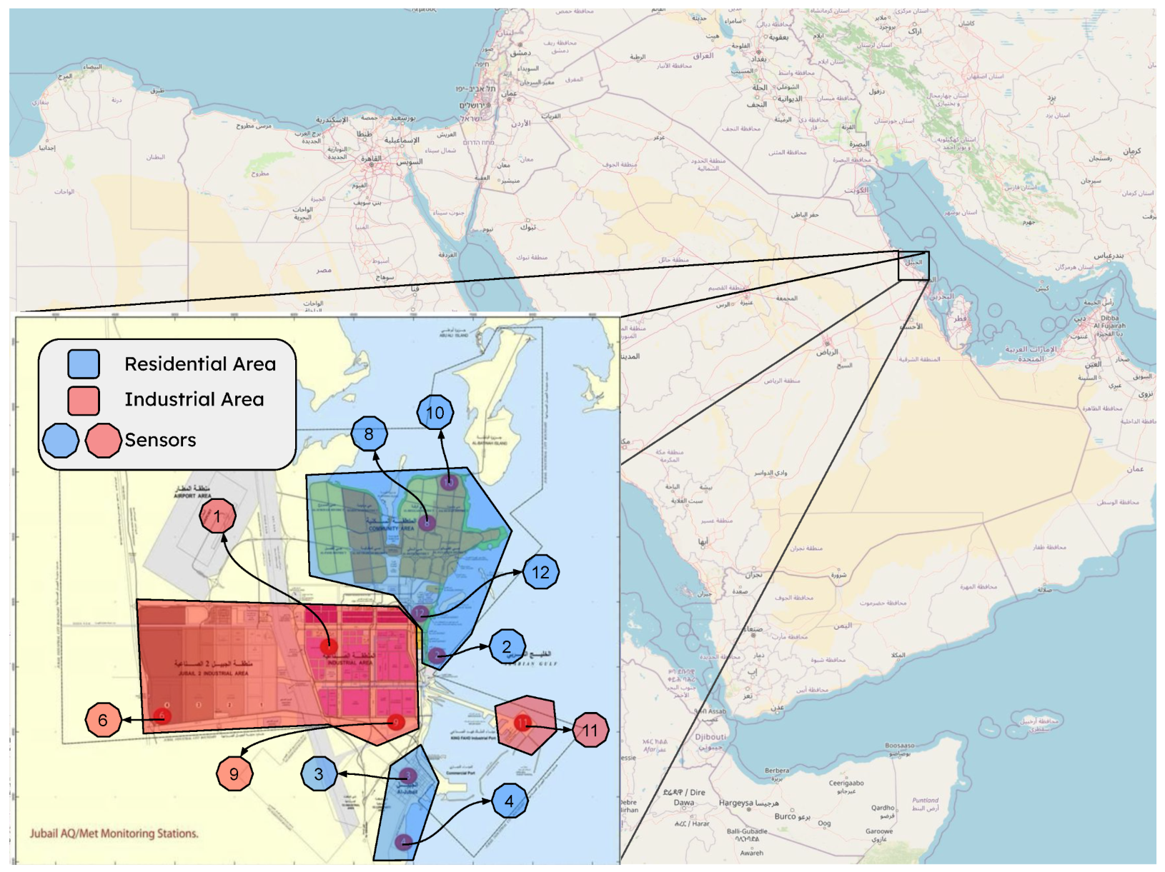
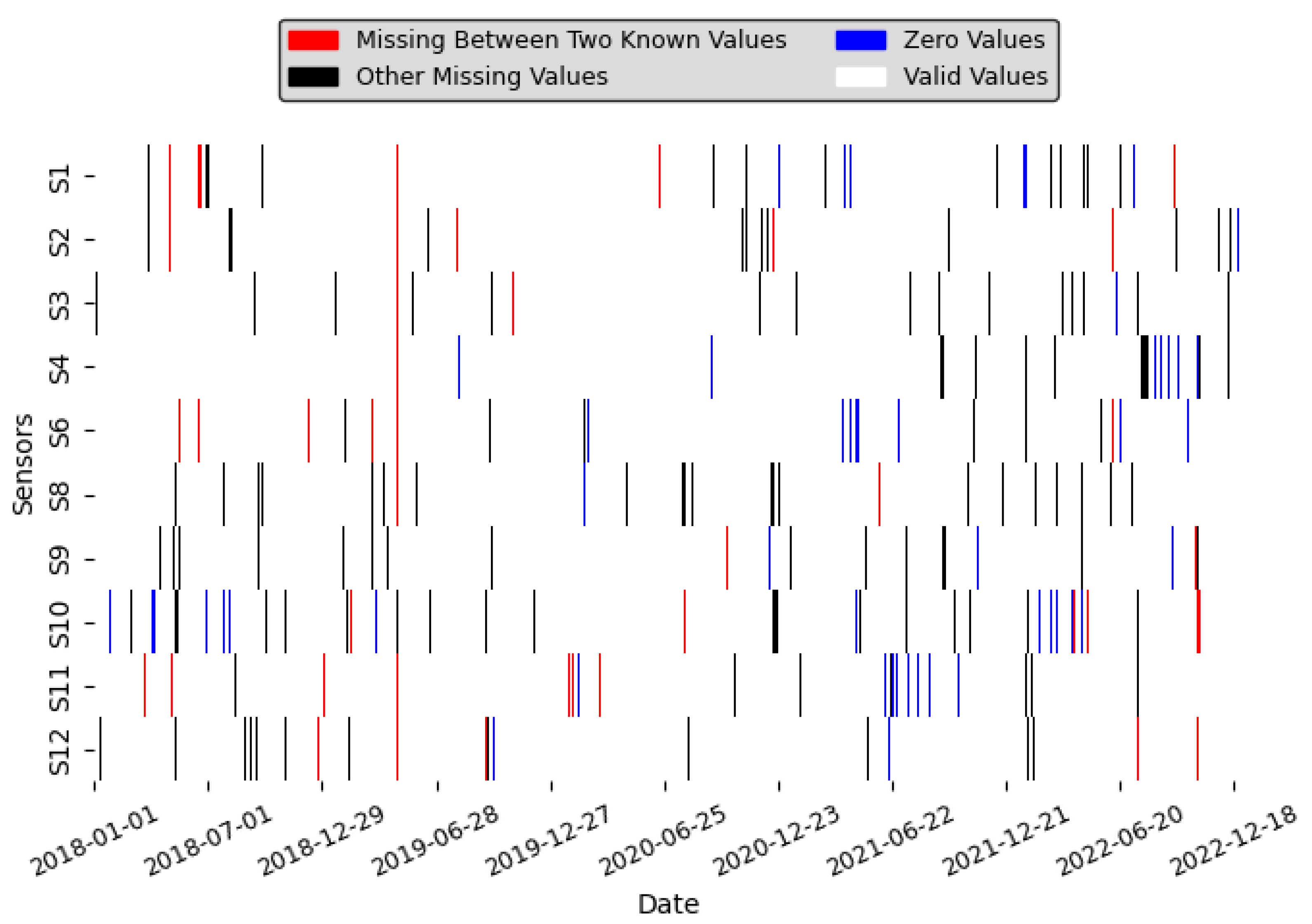
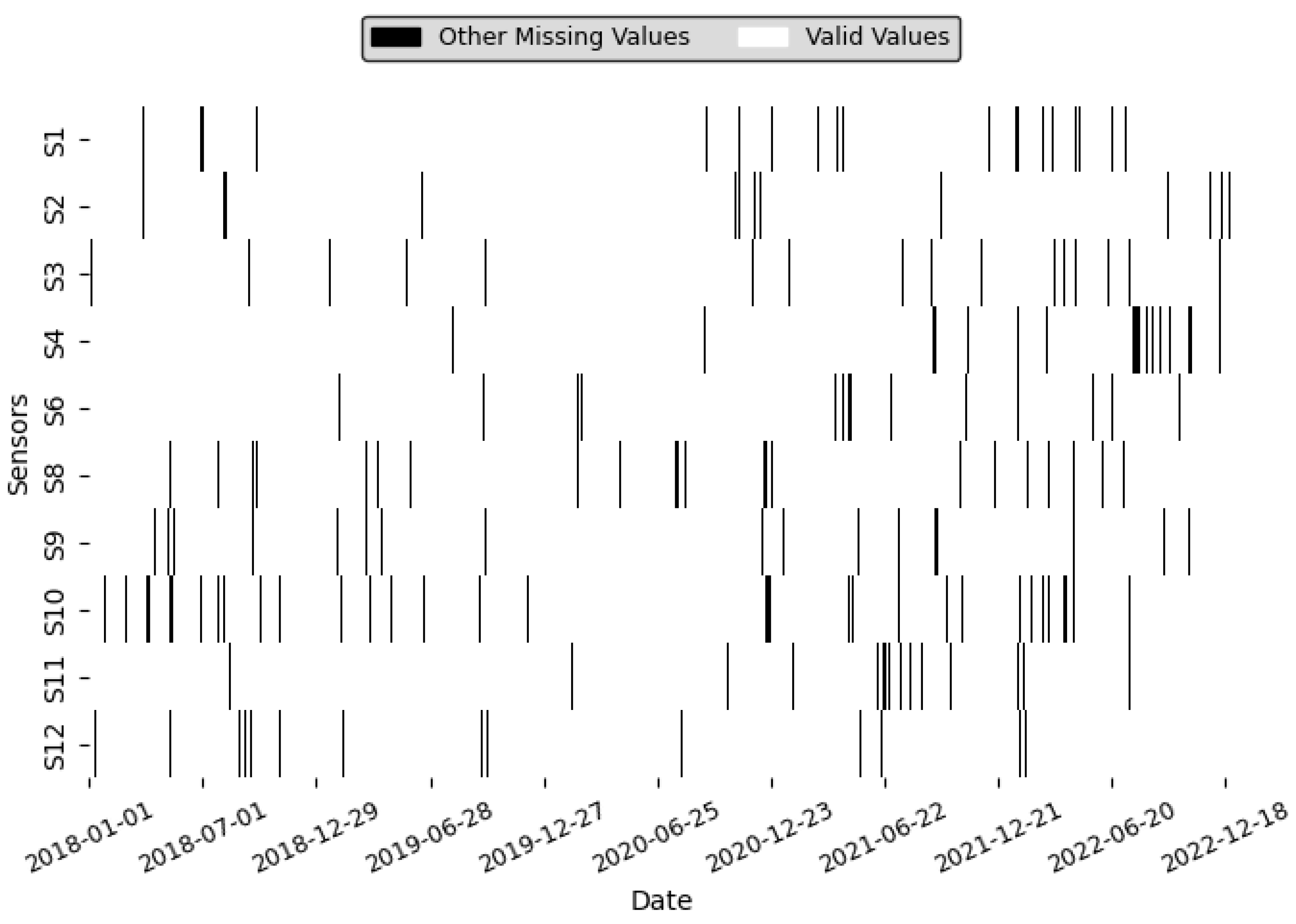
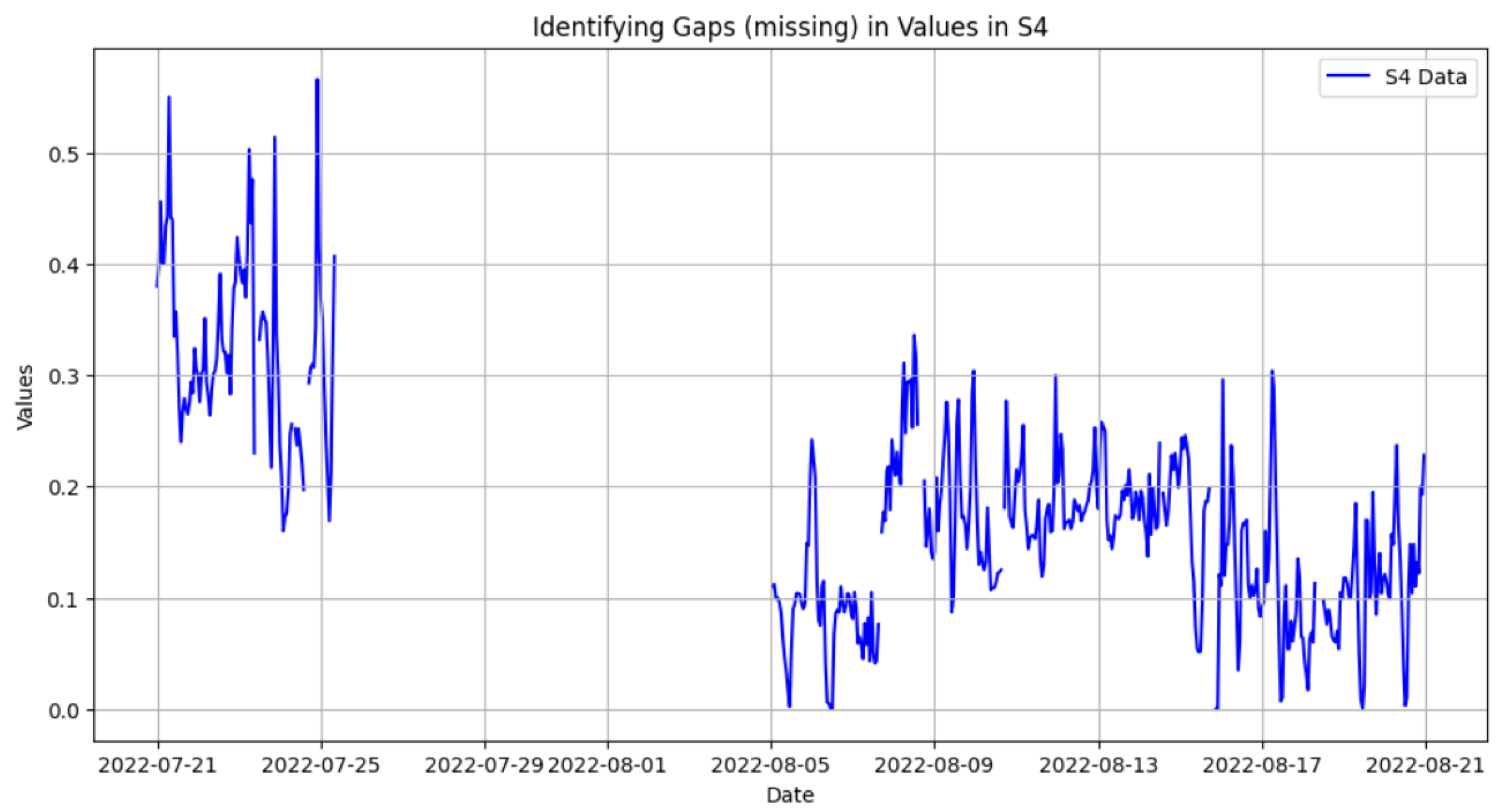
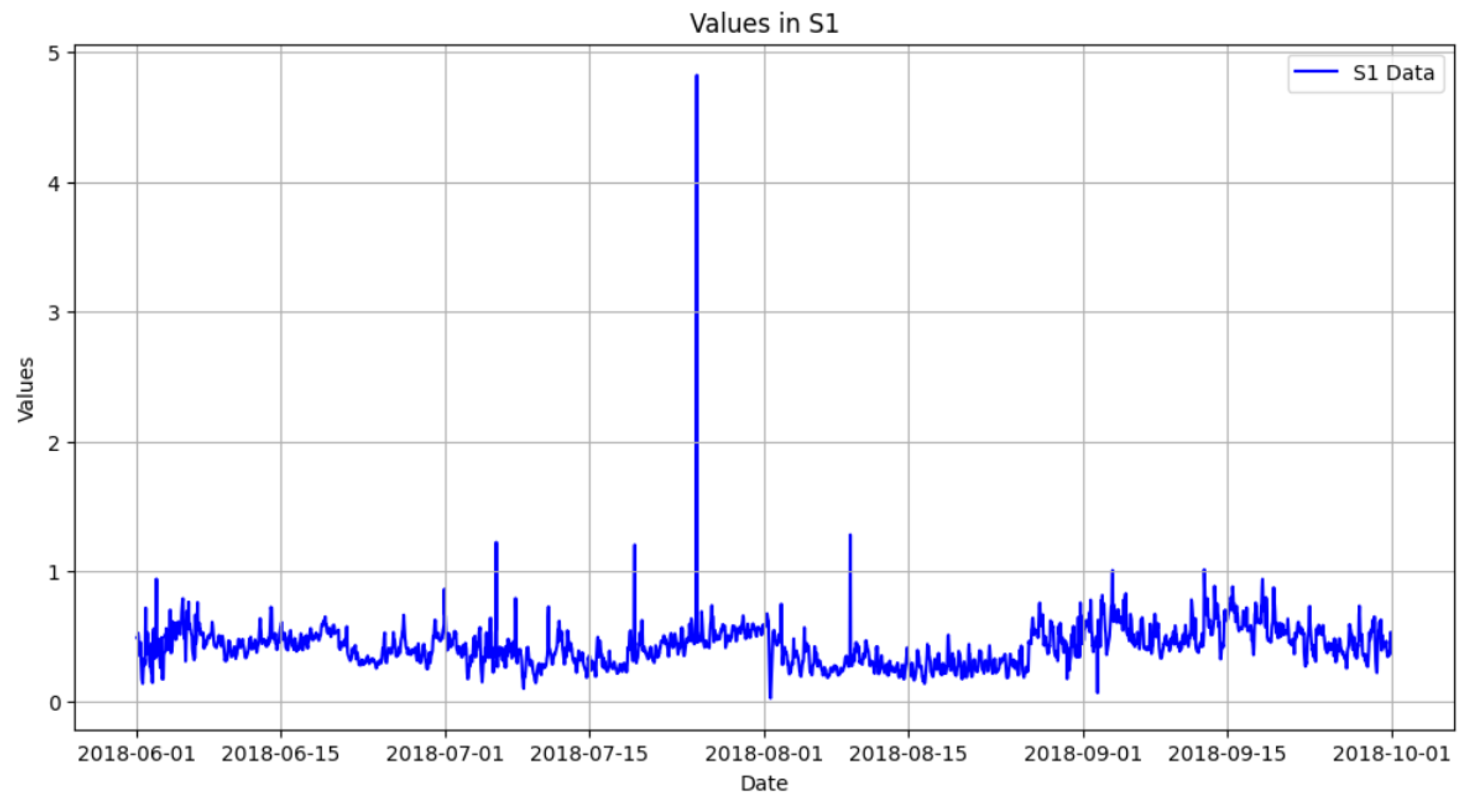
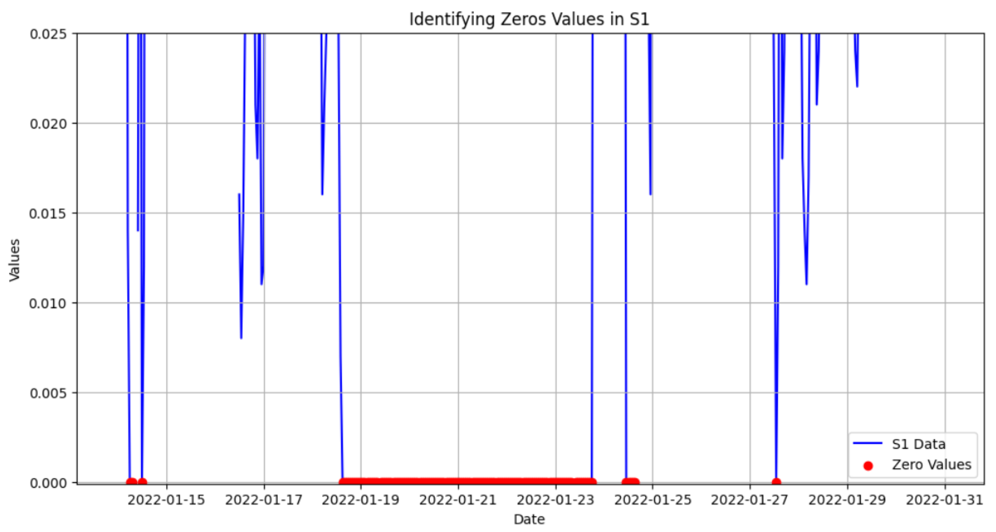
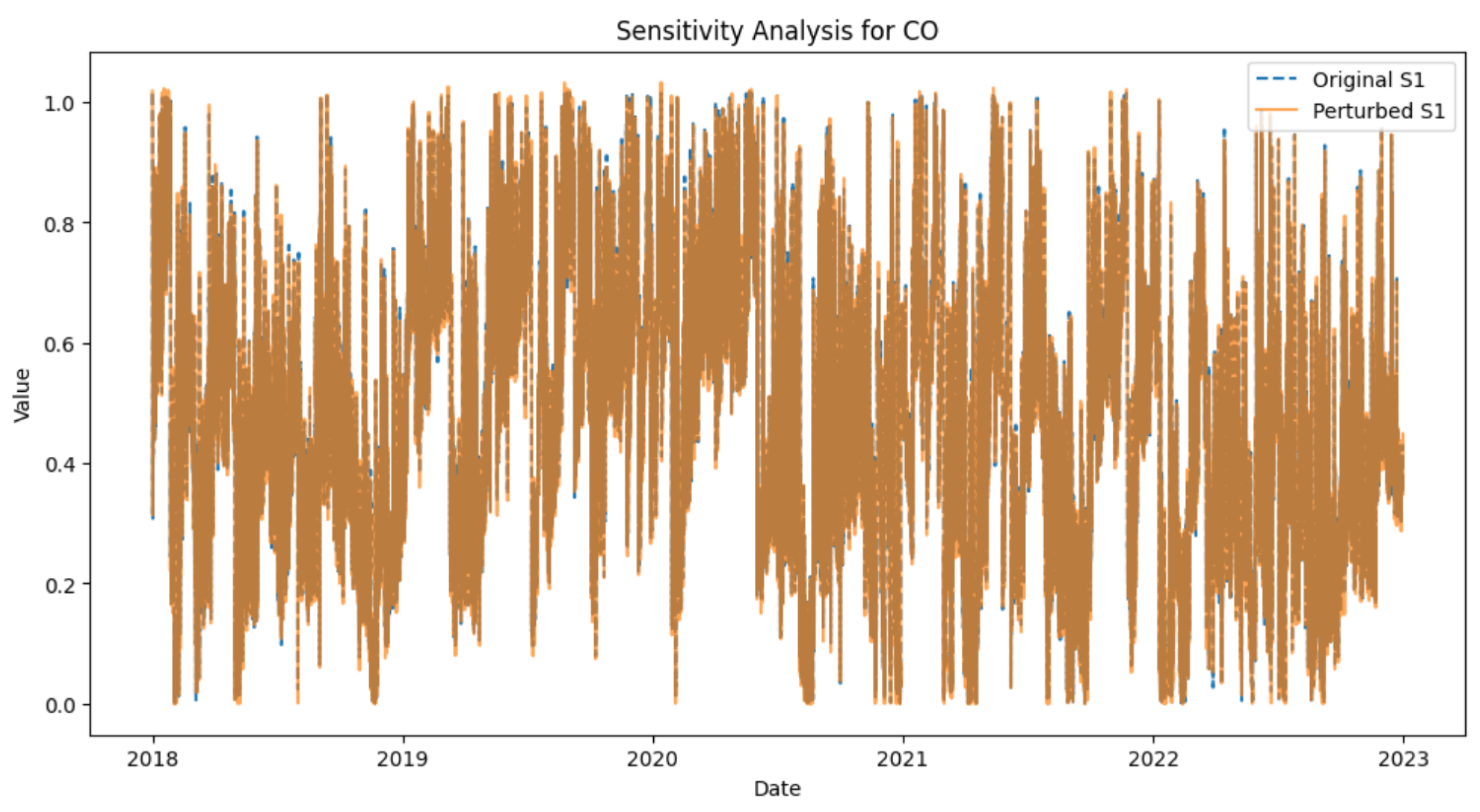
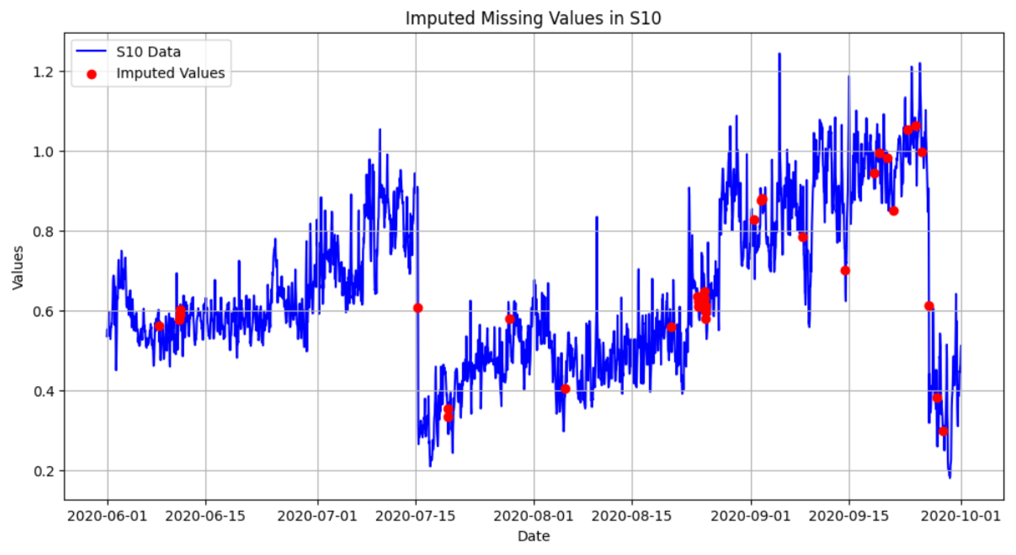
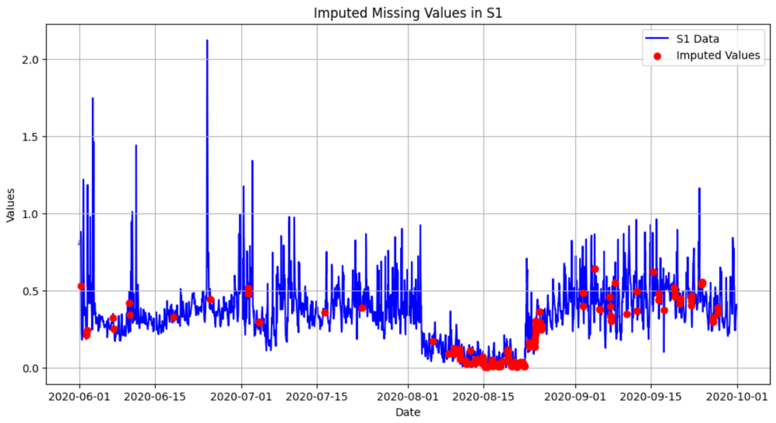