Intelligent Methods of Operational Response to Accidents in Urban Water Supply Systems Based on LSTM Neural Network Models

Highlights

What are the main findings?

• An IoT-based information system has been developed, integrating piezoelectric pressure sensors to collect pressure data in the water supply system, enabling real-time monitoring of the hydraulic network’s condition and using this data for model training.
• Various architectural parameters of the LSTM model have been investigated, including the number of layers, neurons, the use of Dropout layers, the impact of seasonal factors, and the history depth on prediction accuracy.

What is the implication of the main finding?

• The information system allows for the integration of standard devices into cloud platforms for model training, accelerating the process of real-time prediction and simulation.
• The research results, demonstrating the optimal model architecture, can be used in the early stages of training, reducing computational costs during the integration of pressure sensors into information systems and speeding up the model training process necessary for pressure prediction in emergency situations.

Abstract

This paper investigates the application of recurrent neural networks, specifically Long Short-Term Memory (LSTM) models, for pressure forecasting in urban water supply systems. The objective of this study was to evaluate the effectiveness of LSTM models for pressure prediction tasks. To acquire real-time pressure data, an information system based on Internet of Things (IoT) technology using the MQTT protocol was proposed. The paper presents a data pre-processing algorithm for model training, as well as an analysis of the influence of various architectural parameters, such as the number of LSTM layers, the utilization of Dropout layers for regularization, and the number of neurons in Dense (fully connected) layers. The impact of seasonal factors, including month, day of the week, and time of day, on the pressure forecast quality was also investigated. The results obtained demonstrate that the optimal model consists of two LSTM layers, one Dropout layer, and one Dense layer. The incorporation of seasonal parameters improved prediction accuracy. The model training time increased significantly with the number of layers and neurons, but this did not always result in improved forecast accuracy. The results showed that the optimally tuned LSTM model can achieve high accuracy and outperform traditional methods such as the Holt–Winters model. This study confirms the effectiveness of using LSTM for forecasting in the water supply field and highlights the importance of pre-optimizing the model parameters to achieve the best forecasting results.

1. Introduction

In the context of the development of the smart city concept, technical water supply systems are becoming a critical element in ensuring the sustainable transportation and distribution of vital resources. They play a key role in maintaining the stability of the urban environment, meeting the needs of the population, industry, and utilities. However, with the development of social and technological infrastructure, water supply networks not only expand, covering ever larger territories, but also become more complex and branched. Such a structure increases the risk of ruptures and accidents due to equipment wear, uncontrolled loads, or the influence of external factors, such as extreme weather conditions. Such emergency situations lead to serious environmental, economic, and social consequences, including water leaks, environmental pollution, and interruptions in the supply of urban consumers.

Traditional methods of responding to accidents in water supply systems involve detecting failures only after the actual failure, often based on calls received by the water utility dispatch service. This approach is not always effective, since the limited resources of operational repair teams or the remoteness of facilities lead to significant delays in troubleshooting, which increases the average time to restore the water supply. However, with the development of the Internet of Things (IoT) technology, it has become possible to integrate smart sensors into monitoring systems, which allows for collecting data on the state of the hydraulic network in real time. These data can be used to train machine learning models and for the subsequent digitization of the system state, ensuring early detection of potential accidents and increasing the efficiency of their elimination. In this regard, the objective of the study is to evaluate the effectiveness of using a recurrent neural network, namely, one particular variety, the long short-term memory (LSTM) model, in pressure forecasting problems. The scientific article examines the features of obtaining pressure data for training models and studies various architectures and their characteristics to improve the accuracy of pressure forecasting in water supply systems. The studies are carried out on the basis of the water supply system of the city of Gomel (Republic of Belarus), which has a significant length of pipeline networks. The scientific contribution of the article is expressed in the following positions:

(1) The mechanism for obtaining data for training a hydraulic model based on the Internet of Things (IoT) technology using the MQTT protocol is considered. The process of collecting and preparing data is described in detail, including the difficulties and features that affect the quality of machine learning models.

(2) The effectiveness of various neural network architectures used for interval pressure forecasting is studied. An analysis of the optimization of the internal network architecture is carried out, including an assessment of the influence of seasonal factors, the search for the optimal number of neurons in the LSTM model layers, the choice of the forecast horizon, the length of the historical sequence, and the number of training epochs. All these aspects are considered to improve the accuracy and stability of the model when applied to water supply problems.

It is expected that the proposed approach to the selection and optimization of a machine learning model, in particular, LSTM models, will allow for establishing basic parameters for predicting pressure in water supply systems at the training stage. This approach will eliminate the need for the long and resource-intensive processes of searching for optimal hyperparameters, which will significantly reduce the cost of computing resources for model training. This will provide the possibility of the more rapid implementation of intelligent monitoring systems on the scale of large urban water supply networks and will increase their efficiency due to fast and accurate interval forecasting.

2. Related Works

In recent years, the development of machine learning methods, including recurrent neural networks, has significantly expanded the capabilities of time series analysis and forecasting complex dynamic processes. These approaches are successfully applied in various fields, from modeling the microclimate in closed environments [1] to predicting hydrodynamic processes such as tides and water level changes [2]. Predictive models serve as a standard for assessing deviations in process parameters, which contributes to a deeper understanding of individual elements and the system as a whole [3]. The integration of these methods into the management of urban infrastructures, including water supply systems, allows for not only predicting changes in network pressure, but also preventing emergency situations, ensuring more efficient and sustainable resource management. Within the framework of global experience, special attention in this context is paid to improving the best practices used to prevent accidents, as well as assessing their contribution to improving the management and maintenance of water supply infrastructure. Although the focus of this paper is on water supply systems, artificial intelligence algorithms demonstrate high potential for application in related areas such as the gas supply, oil industry, and heat supply. Below, we will consider the main research areas relevant to the problem of pressure forecasting in urban water supply systems based on recurrent neural networks, including LSTM models, solved in this paper.

In the last decade, machine learning methods have been actively used to detect leaks and predict failures in pipeline systems. In particular, Ezechi and Okoroafor (2023) [4] evaluated the effectiveness of recurrent neural networks (RNN) and the k-nearest neighbors algorithm for gas leak detection. Their results showed that RNNs are better able to adapt to dynamic conditions and large amounts of data. Similar conclusions were obtained in works comparing different ensemble models—XGBoost, CatBoost, and LightGBM—in relation to assessing the risk of pipe failure under unstable pressure (Liu et al., 2022 [5]; Fan et al., 2022 [6]). CatBoost and LightGBM demonstrated high accuracy in this context, which emphasizes the prospects for using boosting algorithms in utility networks. For the specific problem of water leak monitoring, Sourabh et al. (2023) [7] proposed an ANN- and SVM-based approach that analyzes pressure and flow time series. They showed that extensive learning on diverse scenarios (different pipe diameters, materials, and conditions) improves the leak detection accuracy. Adding spatial data (geolocation, soil geology) is also effective in identifying patterns related to failure rates (Robles-Velasco et al., 2021 [8]). Traditional hydraulic models can be complemented by intelligent methods, as demonstrated by Momeni and Piratla (2022) [9].

In parallel with classical machine learning methods, deep neural network (DNN) architectures have been widely studied in recent years to solve similar problems. For example, Tsai et al. (2022) [10] developed a leak detection system based on IoT and CNN, achieving an accuracy of over 95%. Robles-Velasco et al. (2021) [8] applied ANN to predict failures given the physical characteristics of pipes, which made it possible to take into account the influence of material and geometric parameters. Liu, Xie, and Song (2023) [11] compared ResNet and classical CNNs, noting that ResNet showed higher training speed and accuracy due to skip connections. Another promising direction is the integration of convolutional networks with graph neural networks (GCN) for modeling the topology of water distribution systems. Liu et al. (2024) [12] demonstrated that GCN-LSTM can simultaneously account for spatial and temporal dependencies, improving the prediction quality of parameters (e.g., pressure) at different points in the network.

Some researchers emphasize that to improve the accuracy of water supply forecasts, it is necessary to take into account not only technical but also socio-economic and climatic factors. For example, Fan et al. (2022) [6] showed that temperature, precipitation, and consumer behavior (income level, location of industrial load zones) can significantly affect the frequency of accidents. Urban population growth and seasonal demand for water increase the load on pumping stations, which increases the risk of leaks, and extreme weather events require rapid and adaptive management. However, most studies focus only on analyzing the consequences of changes in water consumption [13,14], while the problem of identifying factors that could be automatically obtained and used for short-term forecasting remains unresolved. Traditional methods typically rely on information that is difficult to promptly update in real time. For example, demographic parameters and income levels of the population [15,16] are important for assessing the overall demand for water consumption and significantly affect the pressure in the system, but their changes occur gradually and do not reflect instantaneous fluctuations in consumption. Similarly, the structure of urban development [15,16] plays an important role in shaping water supply needs, but its influence is poorly amenable to rapid adjustment, so in real conditions, such data are rarely used for the adaptive management of water intakes [17].

In this context, recurrent neural networks (RNNs), including LSTM and GRU architectures, are of particular importance for time series analysis in water supply systems. Their ability to account for long-term dependencies is particularly useful in predicting seasonal pressure fluctuations or detecting abnormal sharp jumps (Kavya et al., 2023 [18]; Kammoun et al., 2023 [19]). In particular, LSTM efficiently handles data with missing values and allows the model to be flexibly adapted to changing operating conditions (Ki et al., 2020 [20]). In the field of pressure forecasting and accident prevention, hybrid schemes have gained popularity: for example, a combination of 1D-CNN and GRU with multi-head attention (Zhao et al., 2024 [21]) or a combination of LSTM with Informer Framework (Yang & Shi, 2025 [22]). These integrated approaches show high accuracy with large volumes of input data and different forecast time horizons (from several minutes to several hours or days).

An analysis of recent publications shows that deep recurrent models (LSTM, GRU) and their hybrids (CNN-LSTM, GCN-LSTM) demonstrate the highest accuracy in pressure forecasting and anomaly detection in water supply systems. They effectively use high-dimensional time series, take into account spatial dependencies (via GCN or ResNet), and allow for the timely recognition of critical changes [19,21]. However, as noted by Liu et al. (2023) [11], complex architectures require large computational resources and are often focused on a long forecasting horizon. At the same time, the issue of the optimal selection of LSTM hyperparameters for short-term (operational) pressure forecasts in real urban network conditions, taking into account seasonal factors (month, day of the week, time of day), remains insufficiently studied. This study proposes a methodology for constructing a compact LSTM model focused on short-term pressure forecasts and rapid adaptation in potential emergency situations. To accomplish this, we analyze the efficiency of various architectures (number of LSTM layers, Dropout, Dense), evaluate the influence of the season, and compare the obtained results with the traditional exponential smoothing model (Holt–Winters). This approach logically continues the ideas laid down in the works [1,2,3,4,5,6,7,8,9,10,11,12,13,14,15,16,17,18,19,20,21,22,23] and contributes to solving a practical problem—increasing the reliability of water supply in large cities through operational pressure forecasting.

The choice of the LSTM model in this study is due to its ability to effectively account for both short-term fluctuations and long-term pressure trends by storing information over significant time intervals, which is critical for tasks with a pronounced time structure. Unlike the simpler GRU, which can reduce accuracy when working with long sequences, LSTM provides a more accurate modeling of pressure dynamics in urban networks [24]. The use of more complex models, such as Transformer, was limited due to the insufficient data volume and high computational cost of this architecture [25].

Table 1. Comparison of different types of forecasting models.

Characteristic	LSTM	GRU	Transformer
The main mechanism	Information flow control mechanisms	Simplified mechanisms for managing information flow	Self-attention mechanism
Strengths	Effective identification of short-term and long-term dependencies, processing variable length sequences	Computational efficiency, comparable performance to LSTM, faster computing speed	Efficiently identify long-term dependencies over long data history
Restrictions	High computational complexity, need for hyperparameter tuning	Potential difficulties when working with very long sequences, in some cases high instability during training	High computational costs, large number of parameters requiring large amounts of data for training

shows the results of the comparison of the different types of models.

3. Methods

This study focuses on creating a short-term pressure forecasting model for the urban water supply system. This is due to the need for a prompt response to changes in the network, which is especially important for the rapid prevention of emergency situations. Since the hydraulic parameters of the water supply system are constantly changing under the influence of various factors, one of the key features of such forecasting is the use of current pressure data. To compensate for possible seasonal fluctuations, the models include such time parameters as month, day of the week, and hour and minute, which allows for regular changes in the load in the system.

The structure of the study consisted of several consecutive stages. At the first stage, a data collection and exchange scheme was developed, including connecting IoT devices, receiving information from pressure sensors, and transmitting it to a cloud storage system. This stage provided the basis for forming a statistical database and training models. At the second stage, data preparation was carried out: eliminating gaps, normalization, necessary transformations of time series, and dividing statistics into training and test data. At the next stage, the structure of the model class in Python 3.12.8 was created, which included setting up the architecture and activation functions, optimizing the hyperparameters, and establishing the training procedures. The last stage was devoted to training and testing the recurrent neural network (RNN) model using its LSTM variety. The effectiveness of the model was assessed based on metrics such as MAE, SMAPE, MAE, and RMSE.

3.1. Organization of Data Collection for Monitoring Pressure in a Water Supply System

An information system has been developed for the operational monitoring and archiving of the pressure parameters of pumping stations in the water supply system of Gomel (Republic of Belarus). Within the framework of this system, adhering to the concept of the Internet of Things (IoT), a network of interconnected smart devices was deployed that automatically collect, exchange, and process data [26]. 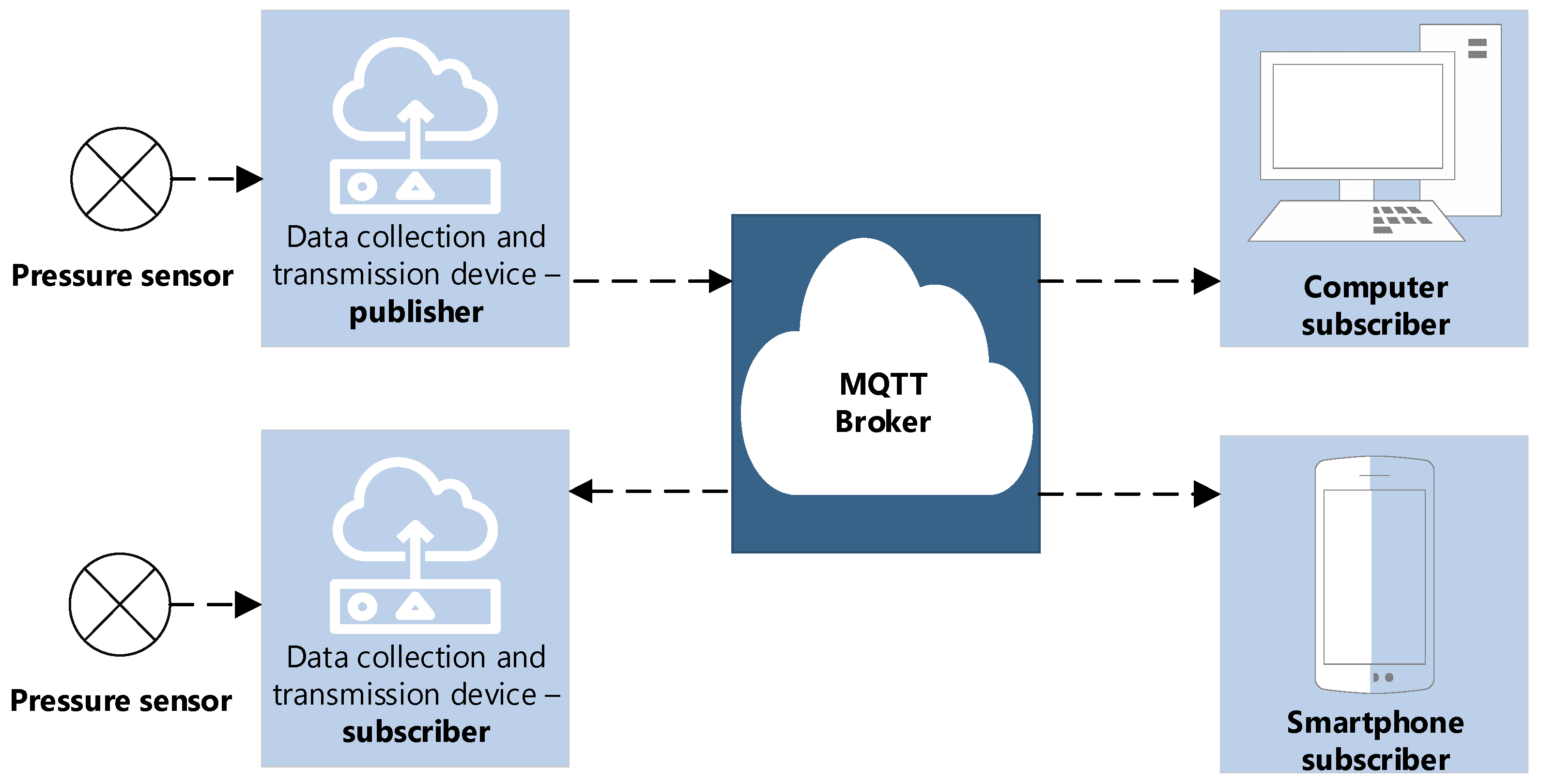Figure 1 shows the diagram used, demonstrating the connection of pressure sensors to data collection and transmission devices that polled these sensors and sent the received information in raw form to the computing server [27]. To ensure the reliability of receiving and transmitting information, a specialized Mosquitto broker (MQTT broker) was installed on the server, acting as a central node. It ensured the coordination of data transmission between data publishers (pressure sensors) and subscribers [28] (personal computers, telephones). The developed architecture facilitated a prompt response to changes in system parameters and the formation of statistical data for the subsequent training of the long short-term memory model.

In the context of this study, the data sources were PD100 piezoelectric pressure transducers of the Russian Oven trademark. This choice was due to the high accuracy of the device, which was critical for the formation of a reliable pressure database at the inlet of the pumping stations. The pressure sensors were connected directly to the pressure gauges (Figure 2b) according to a specific layout on the city map in accordance with the identified water consumption clusters [29]. This made it possible to quickly organize the installation of equipment in the most significant water supply units. It is worth noting that in the absence of pressure gauges, connecting the sensors requires more complex operations that require preparatory welding. RTU-8xx modems from Teleofis (Figure 2a), configured for 5 min measurements and sending messages to the cloud server, served as data collection and transmission devices.

3.2. Features of Data Preparation for Model Training

To train the recurrent neural network (RNN) model, it is important to properly prepare the data. The pressure data in the water supply network was collected using piezoelectric sensors equipped with a telemetry output standardized for the range of 4–20 mA. Raw values in this range were received by the server, which required preliminary transformation before being used in the forecasting model. The current values coming to the cloud server were scaled using linear interpolation to the pressure according to the formula:

$$p=p_{\min }+{\displaystyle \frac{i-i_{\min }}{i_{\max }-i_{\min }}}\left(p_{\max }-p_{\min }\right),$$

(1)

where $p$ is the actual pressure value; $p_{\min }$, $p_{\max }$ are the minimum and maximum pressure sensor values; $i$ is the actual current value; $i_{\min }$, $i_{\max }$ are the minimum (4 mA) and maximum (20 mA) current values.

On the server side, the storage of both raw and transformed pressure data was organized. Raw data included timestamps corresponding to the moment of data collection, as well as current values obtained from the sensors. Transformed data are pressure values calculated using Formula (1) based on the received current. As a result, the database took the form «epoch—pressure», where the first parameter is the timestamp (Unix time) and the second is the transformed pressure value. This approach allowed for storing the data in their original form for further processing and analysis, as well as using ready-made transformed values for the training models. An example of such data is presented in

Table 2. Simplified representation of pressure time series.

Epoch (Unix Time)	Pressure, kPa
1,662,768,000	156
1,662,768,300	167
1,662,768,600	168
1,662,768,900	179

.

The initial statistics then underwent pre-processing, which included removing outliers, filling in missing values, and normalizing features [30]. During the work, a peculiarity was revealed: the data automatically included anomalous values caused by measurement noise, which could be mistakenly interpreted as emergency events. Initially, the quantile data cutoff was used to remove such outliers, but this approach led to the exclusion of real emergency situations, since sharp pressure changes were also classified as outliers. To preserve emergency scenarios while simultaneously eliminating noise, we used median filtering: pressure values were replaced with the median of values in a sliding window during the model training process. This allowed us to preserve significant information about accidents and eliminate distortions caused by noise. Missing values were filled in using linear interpolation from adjacent points, which ensured the integrity of the time series. In this case, min–max normalization was used to bring features to the range from 0 to 1:

$$x_{i.norm}={\displaystyle \frac{x_i-x_{\min }}{x_{\max }-x_{\min }}}.$$

(2)

where $x_{i.norm}$, $x_i$ are the normalized and original features; $x_{\max }$, $x_{\min }$ are the largest and smallest elements of a feature.

Thus, the initial data took the form of a matrix of size T × N. Here, T is the number of time points (or measurements) of the time series, and N is the number of features corresponding to each moment in time. In the example of Table 1, the initial dataset was determined by a single pressure parameter p at time t. In this case, N is equal to 1 and the matrix form of the recording took the following form:

$$\mathbf{A}=\left[\begin{array}{l}{p}_1\\ p_2\\ \cdots \\ p_T\end{array}\right].$$

(3)

In this study, the Keras library in Python [31] was used to train the long short-term memory (LSTM) model. One of the features of LSTM training is the need to represent the input data in a format that takes into account the temporal structure of the sequence. In this training, the input data are represented as a three-dimensional tensor, where the first axis is the number of results (samples) in the data; the second axis corresponds to the duration of the time interval or window that determines the structure of the history, the pattern tracked when predicting pressure; and the third axis denotes the number of features that are used to predict future indicators. The transition of the original matrix A to a multidimensional format to form the input tensor in the LSTM model included the following steps:

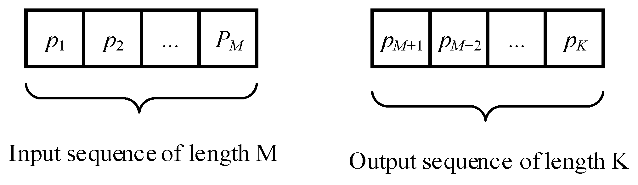
1. The depth of the observation history M was determined, which is one of the parameters of further research, which was selected depending on the accuracy of pressure forecasting (Figure 3). This parameter determines the size of the time window through which the model can «see» changes in the feature over a certain period of time. The depth of the history M allows the model to take into account the influence of past values on the forecast of future values of the output pressure sequence.

2. The optimal forecast horizon of length K was determined (Figure 3). The minimum forecast error at each step of the interval window and the average error of the resulting sequence served as the criterion.

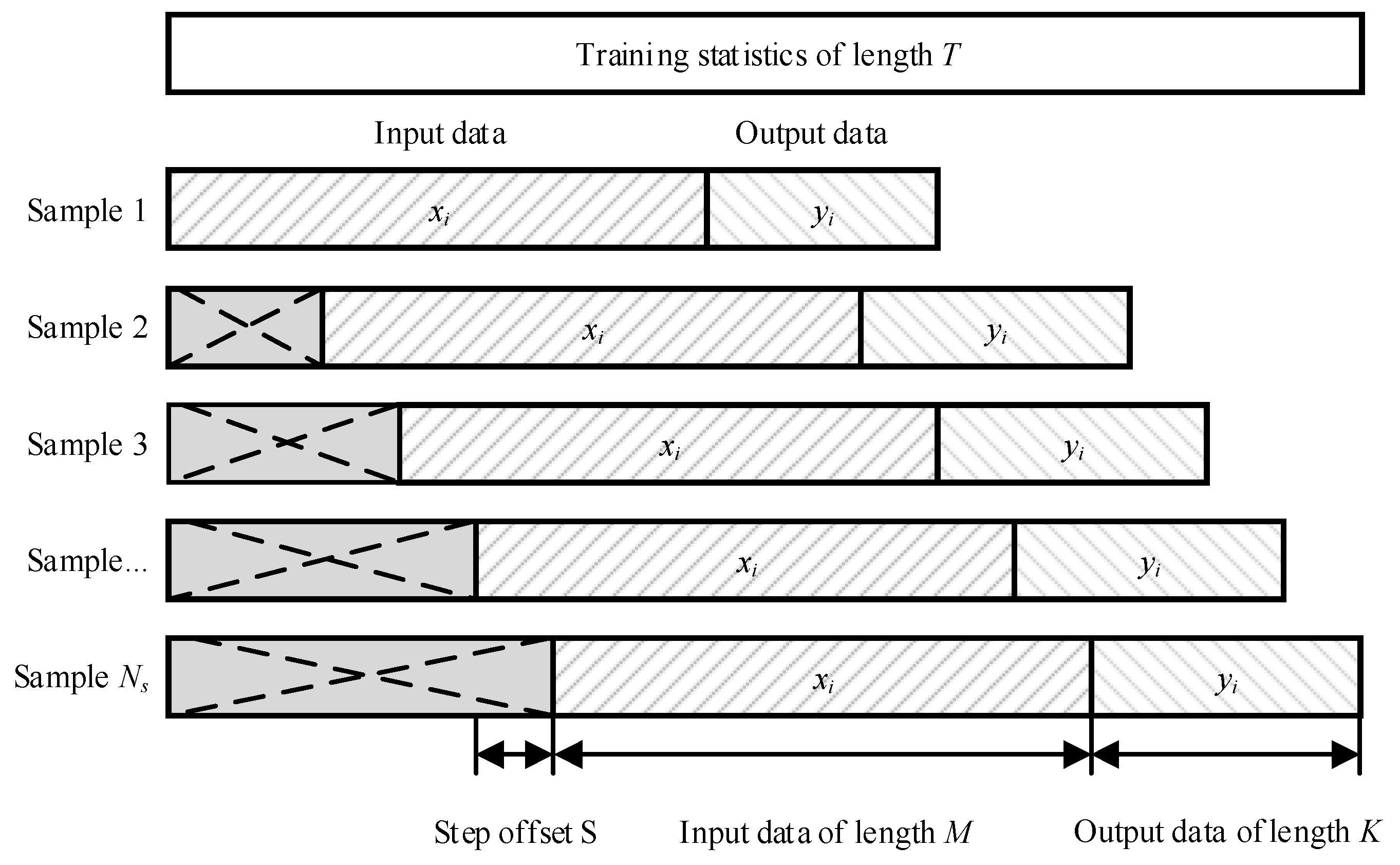
3. The study used various architectures to extract additional factors from the original timestamp (epoch). In particular, such features as minute, hour of day, month index, day of the week type (working or weekend) were additionally extracted. This expanded the original matrix, increasing the number of input features. For each of these features N, a set of time windows of length M was formed, extracted from the original matrix A. The number of such windows was T − M. Further, each of these windows became a sample of dimensions M × N, that is, it contained M observations for each of the N features. In total, T − (M + K) datasets were obtained for training the model (since for each sample it is necessary to have a corresponding output sequence of length K), which determines the number of samples in the three-dimensional tensor.

4. To increase the volume of training data, the rolling window approach was used [32,33]. This method involved forming a set of overlapping sequences, which was achieved by shifting the time series by a given interval (Figure 4). This significantly increased the sample size for training the model. For the initial training data with the number of observations T, the shift step S was specified. Then, for each i-th position of the window with the shift step S = 1, the data samples are in the range $1\le i\le N_S$, where $N_S=T – (M+K)+S$ is the possible number of observations. The training matrix A will contain $a_{i,j}$ elements, where i = 1, 2, …, $N_S$; j = 1, 2, …, M + K.

5. Matrix A was divided into two parts, defining the input data X with elements, where i = 1, 2, … $N_S$; j = 1, 2, …, M; and the output (target) data Y with elements, where I = 1, 2, …, $N_S$; j = M + 1, M + 2, …, M + K. The resulting matrix was reduced to a tensor form, taking into account the number of features of the model:

$$T=\left|A_1,A_2,\dots ,A_i\right|,$$

(4)

where $A_i$ is the input layer matrix of the neural network and has dimensions M × N, where each column represents the i-th subsequence of length M for each of the N features in the time series. Similarly, the output layer of the matrix has dimensions, where each column contains information about K prediction values for each of the P parameters. In this study, one pressure parameter was predicted.

3.3. Features of Assessing the Effectiveness of the Learning Process

At the training stage, the search for optimal model parameters was carried out, such as the history length (M) and prediction depth (K), the number of neurons in the layers of the long short-term memory model (NLSTM). The main goal was to find the LSTM architecture that would provide the maximum accuracy of hydraulic pressure forecasting [34,35]. To assess the quality of the predictive model, the cross-validation method was used, namely, block cross-validation [36]. This method is based on dividing the time series into non-overlapping blocks using a sliding window with a given step. Instead of repeatedly training the model on different data blocks, the model was trained once using the initial architecture settings, which were then changed to find the best configuration. After that, the effectiveness of the model was assessed on the test set. The procedure for assessing the quality of the learning algorithms used in these studies included the following:

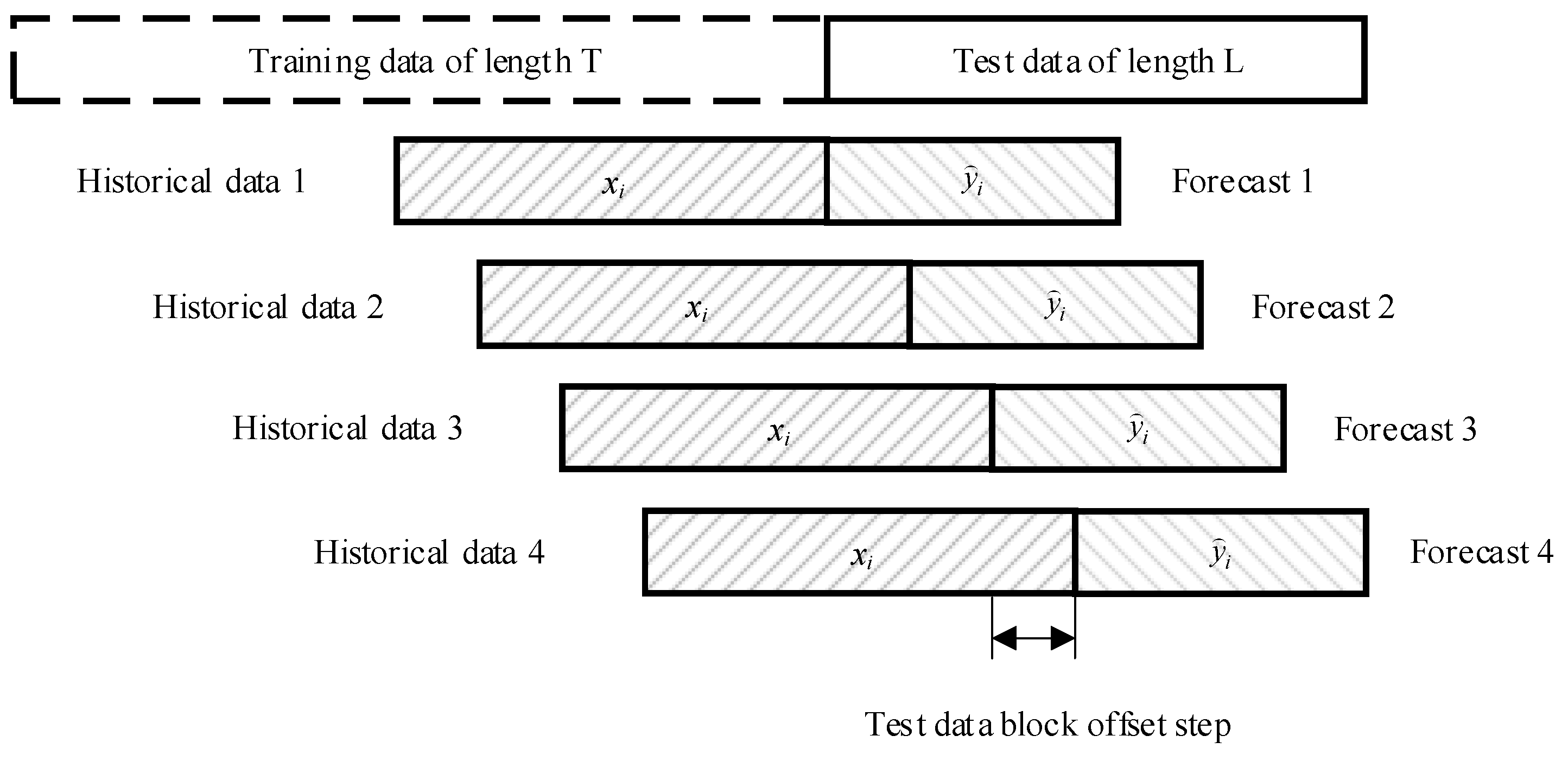
1. Splitting the data into training and test samples: a time series of length T + L (Figure 5) was split into a training sample of length T and a test sample of length L in a ratio of 70% to 30%.

2. Dataset generation: In the forecasting process, a sliding window method with a given step was used to obtain new test data [32]. For each time step t (starting from the first element of the test sample to the end of the time series L), a data block of length M (data history) was used as input and the next K elements were used as the target variable. This formed a dataset of size (T − M − K + 1) × (M + K), where each row contains one set of input and output data (Figure 5).

3. Prediction for a given interval: At each step t, the model made a prediction for a given interval ahead K. The results of the predictions were saved for further analysis.

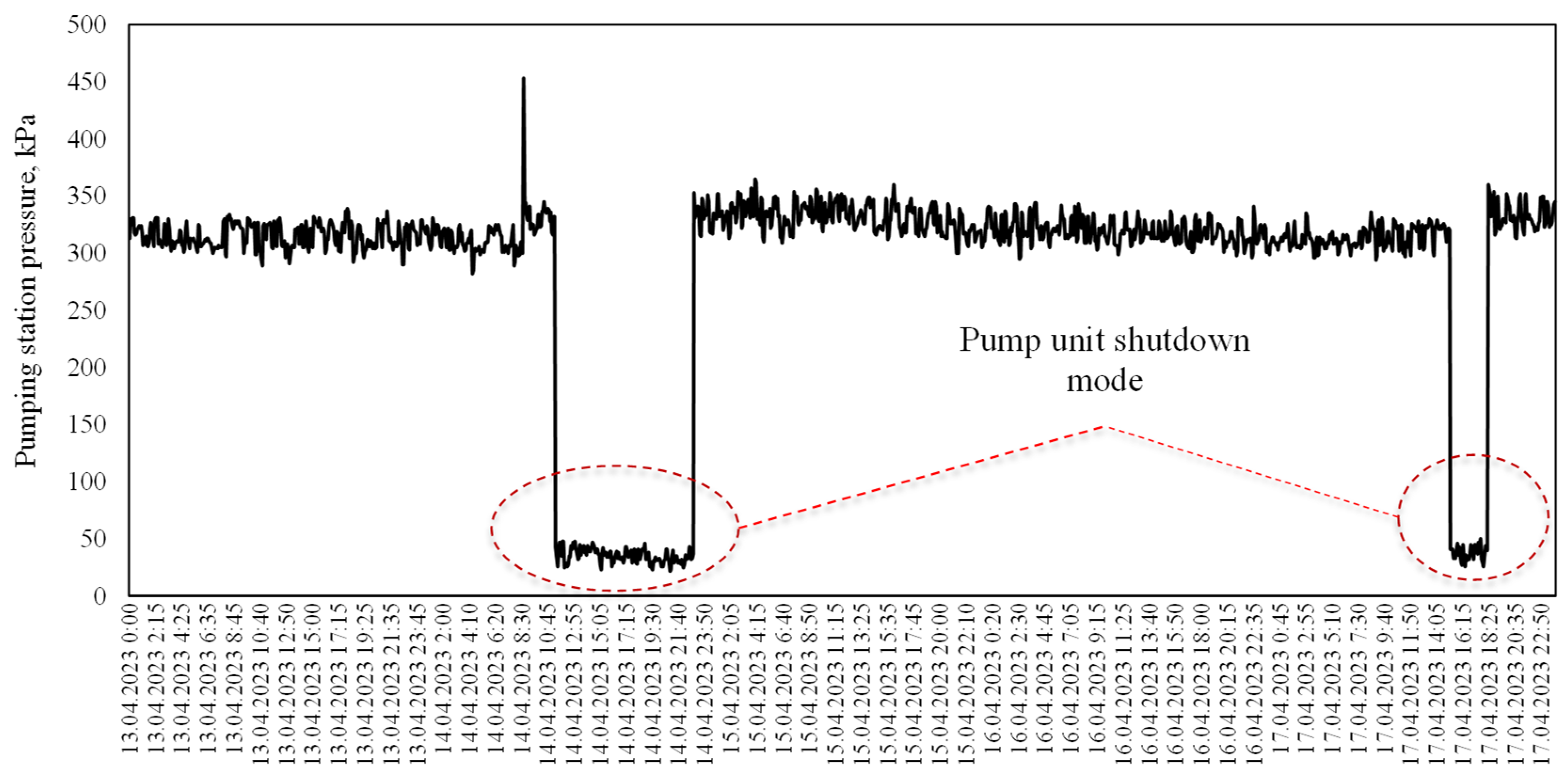
4. Model quality assessment: The obtained predictions were compared with real observations. A distinctive feature was the assessment of both the average error at each step of the block displacement t over the entire depth of the forecast K, and the calculation of the average error of all predictions. In the studies conducted, classical metrics were used to assess the quality of the pressure forecasting model: MAPE (mean absolute percentage error), MAE (mean absolute deviation), and RMSE (root mean square error). Despite the widespread use of MAPE, this metric does not effectively cope with zero values, which is typical for scenarios related to an emergency pressure drop or the on/off modes of pumping stations (Figure 6). In such cases, MAPE gave a distorted estimate due to the mathematical uncertainty that occurs when dividing by zero.

To solve this problem, the SMAPE (symmetric mean percentage error) metric was used as an alternative, which works more stably in such conditions, since it excludes infinite values and gives a more correct assessment of the accuracy of the model at zero pressure values [37]:

$$\mathrm{SMAPE}={\displaystyle \frac{1}{n}}{\displaystyle \sum _{i=1}^n\frac{\left|y_i-{\stackrel{⌢}{y}}_i\right|}{\left(y_i+{\stackrel{⌢}{y}}_i\right)/2}}.$$

(5)

where $y_i$ is the actual value at the i-th moment in time; ${\stackrel{⌢}{y}}_i$ is the predicted value at the i-th moment of time; $n$ is the number of observations.

3.4. Finding the Optimal Architecture and Hyperparameters of the LSTM Model

The goal of the study was to find an LSTM model architecture that would ensure high forecasting accuracy and efficient use of computational and information resources during training. To achieve these goals, various combinations of hyperparameters were used before training. The search for the optimal model structure included the following stages:

(1) Assessing the impact of adding additional layers to the LSTM model: We studied how an increase in the number of layers affects the accuracy of the model and its ability to generalize.

(2) Assessing the impact of parameters that determine seasonality: We analyzed the effectiveness of adding seasonal parameters.

(3) Assessing the impact of the number of neurons in model layers: We studied the dependence of the model accuracy on the number of neurons in hidden layers.

(4) Assessing the impact of the amount of historical data and forecasting range: We analyzed the effect of increasing the volume of training data and further forecasting steps on the accuracy of modeling.

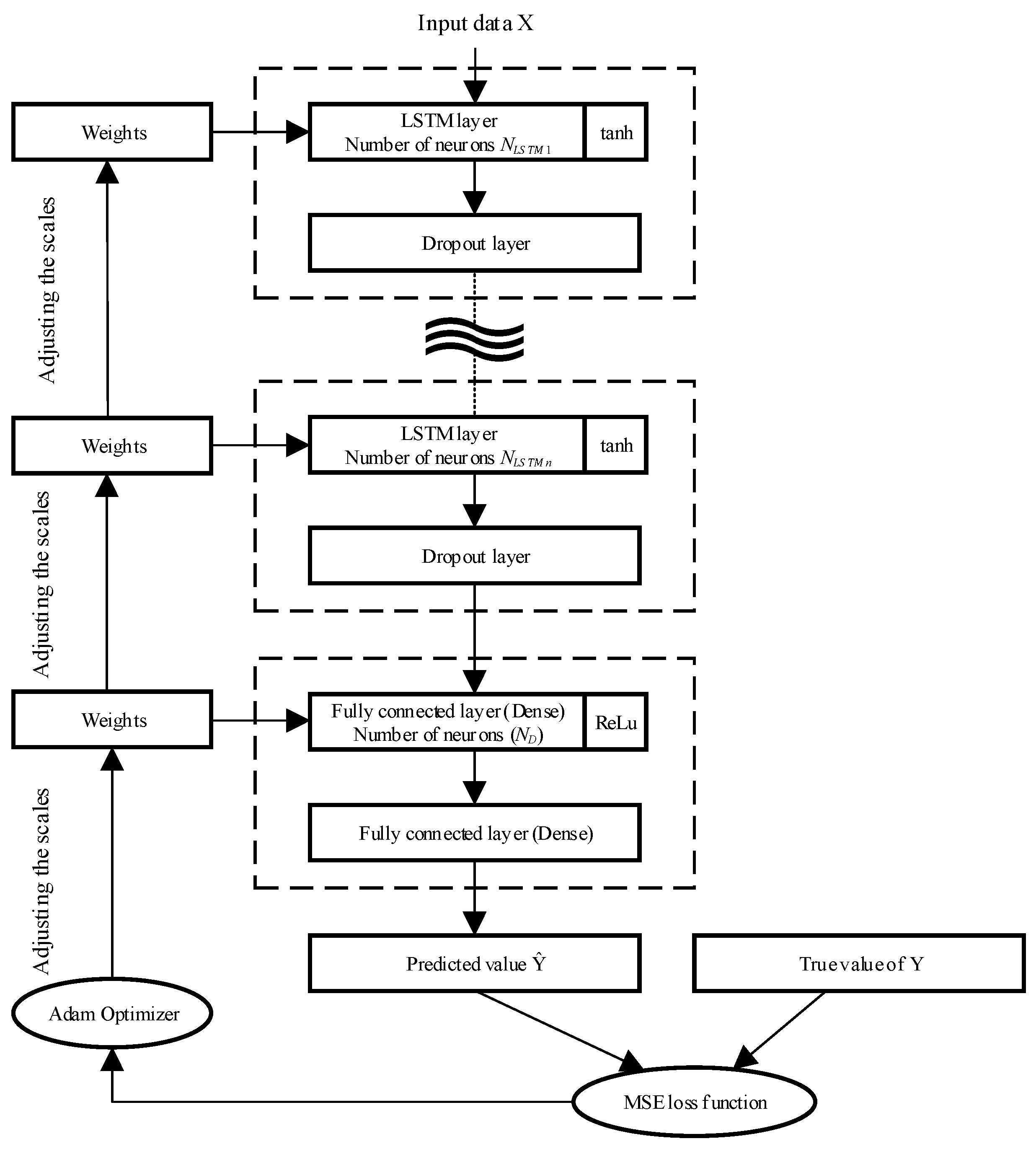
Figure 7 shows a general view of the structure of the long short-term memory model and the relationships between the layers, the network, and the optimization function of the model under study.

The model was tested on statistical data presented by 5 min discretization of the input pressure of the booster pumping station on Artilleriyskaya Street in Gomel for the period from 17 February 2023 to 16 March 2023. The size of the original statistics was [13,398, 2], where the first parameter determines the generated number of observations; the second determines two features: epoch, pressure. One of the possible limitations of this study is the relatively short time interval of the data used for model training, which may not fully reflect long-term seasonal changes in the water supply system. However, it is important to emphasize that this study is not focused on long-term forecasts, but is designed to quickly predict pressure changes in the urban network. In this regard, the main focus is on the latest relevant data, and seasonal parameters such as month, day of the week, and hours and minutes of the day are used in the process of additional training to improve the quality of the model. In future studies, it is possible to expand the time range of the data, which will allow for a more detailed study of the effect of a large dataset on the model quality metrics.

4. Results and Discussion

4.1. Optimization of the Internal Architecture of the Neural Network

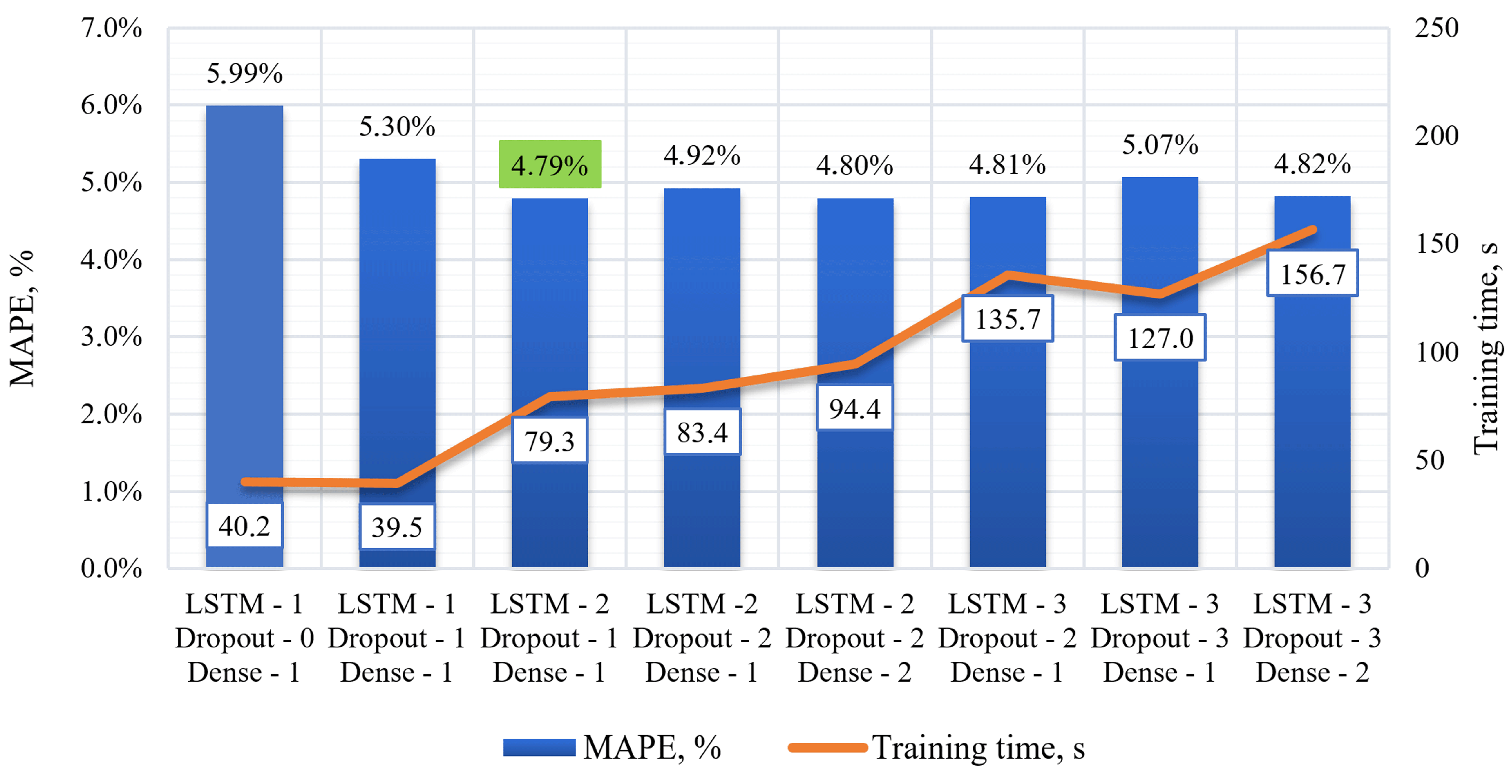
The study tested the impact of additional layers on the model performance. For this purpose, the basic architecture was used, within which the following parameters were fixed: the number of neurons in the LSTM layers and the fully connected layer was fifty; the number of historical observations fed to the model input was twelve; the length of the output sequence, the number of predicted values, was twelve; and the number of input parameters was one (pressure with 5 min discretization). These parameters were selected for the initial setup of the model, after which various configuration options were tried to assess their impact on the forecasting accuracy. In total, seven different architectures with different combinations of the number of LSTM, Dropout, and Dense layers were considered [38,39]. The results of the model performance evaluation are presented in Figure 8.

The study revealed the following:

(1) Increasing the number of LSTM layers to two–three improves the forecast quality and reduces the MAPE, SMAPE, MAE, and RMSE metrics compared to a single-layer LSTM architecture.

(2) Adding a regularization layer (Dropout) improves the model performance. Models with one or two Dropout layers show a lower forecast error compared to models without adding Dropout layers.

(3) Adding additional fully connected layers (Dense) does not always improve the model performance. In this study, models with one Dense layer show better results compared to models with two Dense layers.

(4) Model training time increases with the number of layers and model dimensions. Models with more layers and parameters require more time to train. The model with three LSTM layers, Dropout, and Dense without changing the forecast quality on 20 epochs required twice as much time for training compared to the model consisting of two LSTM layers and one Dropout and one Dense layer. Based on the analysis, we can conclude that the optimal model has two LSTM layers, one Dropout layer, and one Dense layer. The error of the given model on the test data was MAPE = 4.79%.

4.2. Evaluation of the Impact of Seasonal Components on the Efficiency of the Model

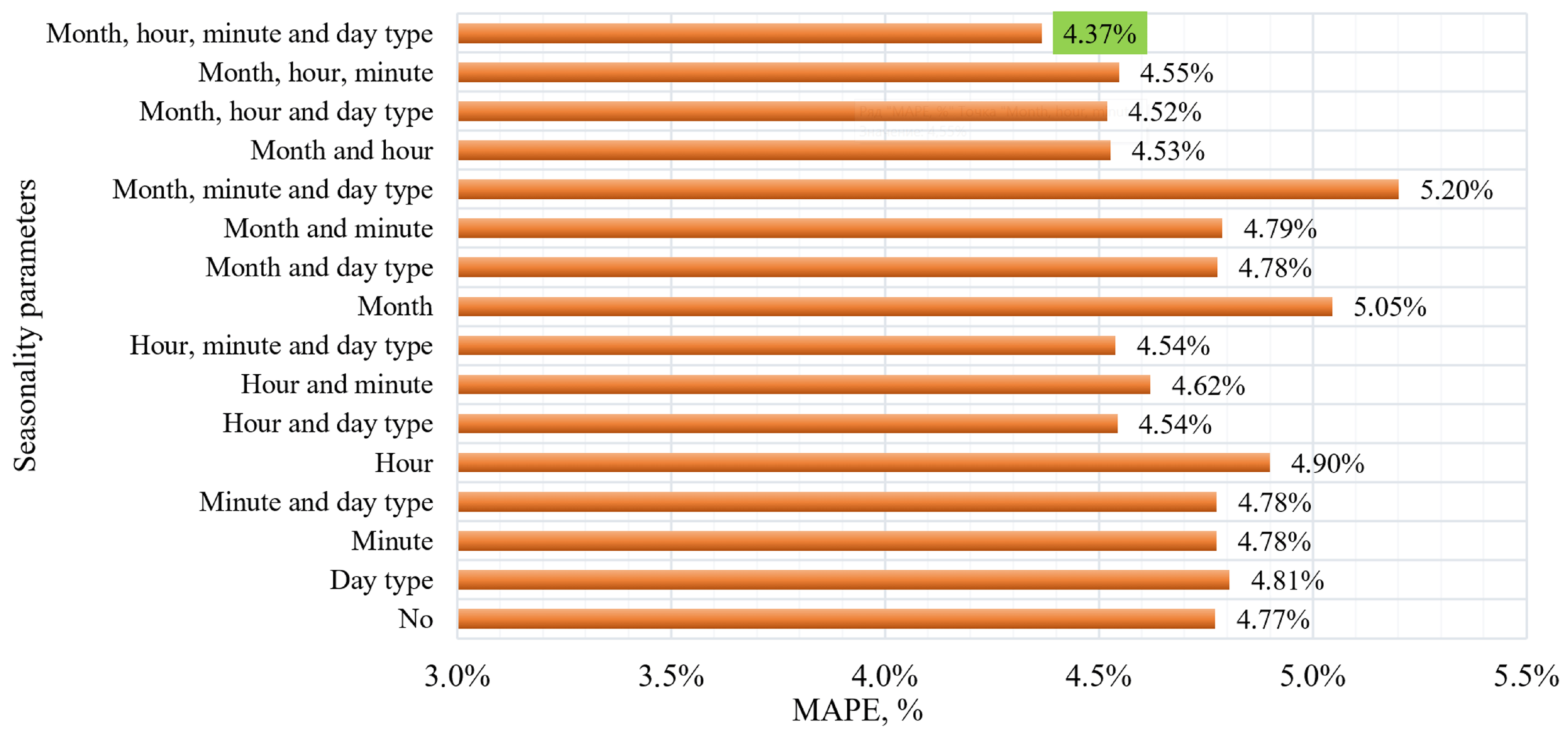
The influence of seasonality parameters on the quality of the LSTM model was studied by adding various combinations of time factors to the input layer of the recurrent neural network. To form such factors, we automatically extracted them from the timestamp (Unix time) recorded along with the pressure data. In addition to the pressure itself, the training set included the following: month number; hour and minute of the day; type of day of the week (working/weekend). To assess the influence of each factor, we sequentially included different combinations of these time parameters in the LSTM model. The training data were collected over two months (September and October 2022), so the “month” factor varied only within two values, which does not allow for full disclosure of annual seasonality. In real operation, this can be compensated for by continuously retraining the model as new data arrive so that it takes into account more time intervals. The “day type” factor in this set also had little variability (only working days and weekends, excluding holidays). Holidays and pre-holiday days were not included in the training set. However, the results shown in Figure 9 show that including different combinations of seasonality parameters affects both the quality of forecasts and the training time of the model.

The analysis results show that in the case when the input statistics did not take into account seasonal factors, the model showed the following results: MAPE—4.77%, SMAPE—4.71%, MAE—8.0 kPa, RMSE—10.3 kPa. Adding the day type as the only seasonal parameter led to a slight increase in MAPE to 4.81%, while SMAPE remained at 4.71%. Adding the minute as the only seasonal parameter increased the MAPE and SMAPE values to 4.78%, and MAE—to 8.1 kPa. Using the minute and day type together increased the training time, but did not lead to a significant improvement in the metrics. Taking into account the hour of day in the model increased MAPE and SMAPE to 4.9%, and also increased MAE and RMSE. The best result was achieved when using all four parameters: month, hour, minute, and day type. This resulted in a MAPE of 4.37%, SMAPE of 4.34%, MAE of 7.4 kPa, and RMSE of 9.4 kPa.

There are several key findings from examining the impact of seasonal components on model performance:

(1) Impact of Seasonality: Including seasonality parameters such as month, hour, minute, and day type in a model improves its predictive ability. Overall, models that include these parameters perform better on all evaluation metrics than models without seasonality parameters. This may be because these parameters help the model capture structure in the data that would be invisible without them.

(2) Training Time: Including more seasonality parameters increases the training time for the model, which is due to the larger number of parameters required to process and train the model. However, it is important to note that despite the increased training time, models with more parameters generally perform better predictively.

(3) Optimal Combination: The lowest MAPE, SMAPE, MAE, and RMSE scores are demonstrated by the model that includes all four seasonality parameters: month, hour, minute, and day type. This indicates that using all of these parameters together results in improved forecast accuracy.

It is worth noting that training the model with seasonal components does not change the procedure for obtaining information from primary converters and does not increase the volume of the database stored on the server. Information about the month, hour, minute, and day type is extracted through the Unix timestamp transformation. This allows seasonality to be taken into account in the data without the additional accumulation of information.

4.3. Finding the Optimal Number of Neurons in LSTM Model Layers

The choice of the model configuration is based on the grid search method, which is used to determine the optimal number of neurons in the LSTM and Dense layers of the neural network [40,41,42]. In accordance with this method of model training, an algorithm for the cyclic enumeration of all possible combinations of hyperparameters is implemented. To enumerate various combinations in each layer, a list of neurons for each of the three layers of the model (two LSTM layers and one Dense layer) with values of 50, 150, and 250 was formed. In the conducted study, 21 models were trained with a total time cost of 110,019 s (30.6 h). During the study, it was noted that an increase in the number of neurons in the first and second LSTM layers leads to a significant increase in the model training time. However, no corresponding improvement in the quality of the model forecasts is observed. This confirms the assumption that the complexity of the model does not always correlate with its performance. In connection with the above observations, it was decided that the cyclic enumeration of parameters would be stopped after reaching the specified configuration. 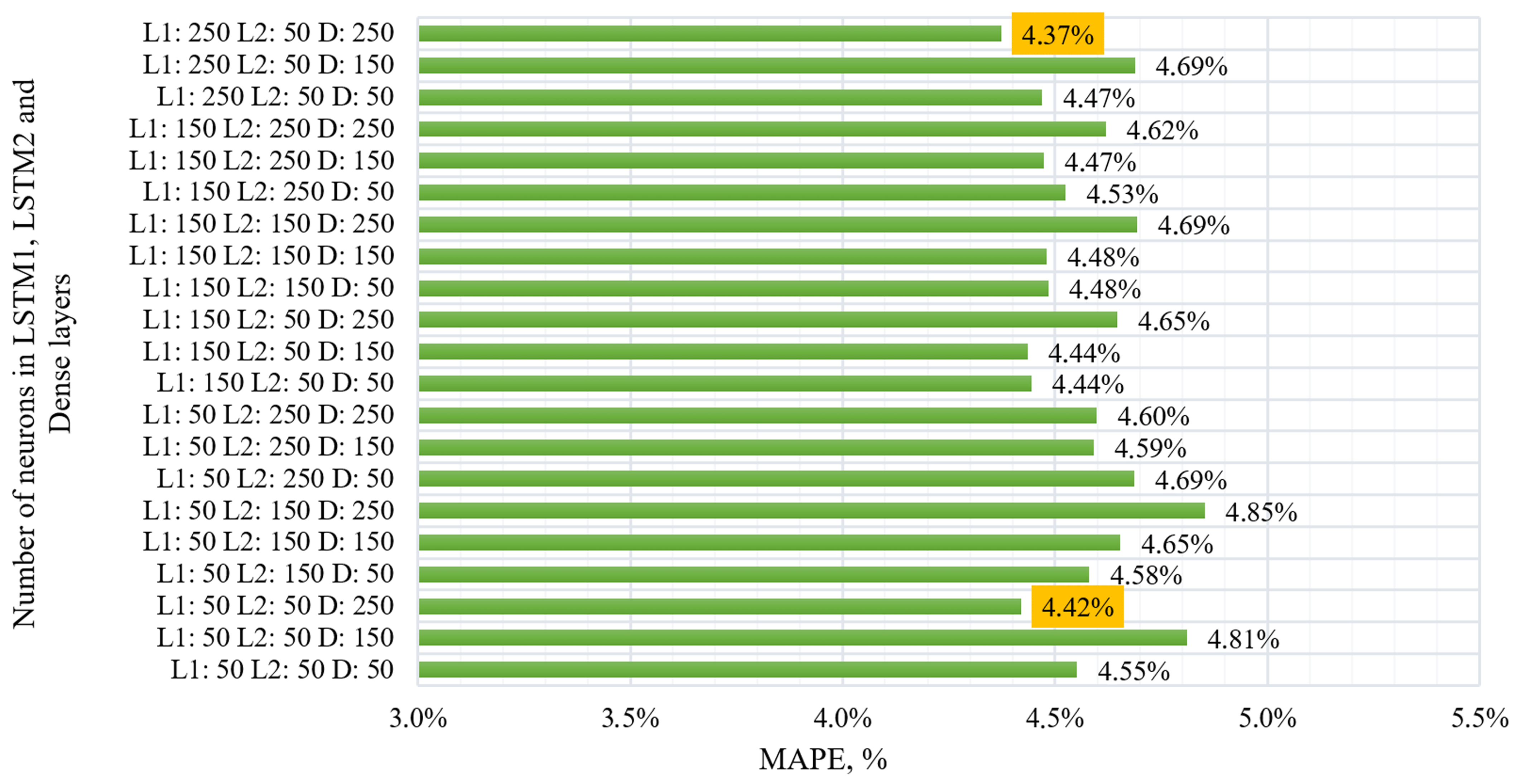Figure 10 shows the distribution diagram of the MAPE forecast error indicator when changing neurons in the two LSTM layers and one Dense layer model.

According to the obtained results, the following are indicated:

(1) The error rates vary in a small range. This indicates that changing the number of neurons in each layer does not lead to a significant improvement or deterioration in the accuracy of the forecast. The lowest error rates are observed in experiments #3 and #21 (L1 = 50, L2 = 50, D = 250 and L1 = 250, L2 = 50, D = 250, respectively). This may indicate that increasing the number of neurons in the Dense layer with a relatively small number of neurons in the LSTM layers, taking into account the resource costs for training, may be more effective for the task under study.

(2) The training time of the models varies significantly and, as a rule, increases with an increase in the number of neurons. The fastest learning occurs with the smallest number of neurons (L1 = 50, L2 = 50, D = 50); the slowest occurs with the largest (L1 = 150, L2 = 250, D = 150 and L1 = 150, L2 = 250, D = 250).

(3) In this problem, increasing the number of neurons in the layers does not always lead to an improvement in the forecast accuracy. At the same time, the training time increases significantly, which can be critical with limited computing resources. Based on these results, we can conclude that the optimal configuration is a model with 50 neurons in the LSTM layers and 250 neurons in the Dense layer as the most optimal in terms of the ratio of forecast accuracy and training time. In some cases, the growth of neurons in the first LSTM layer leads to an improvement in the quality of the model. With limited resources, the LSTM and Dense layers can be reduced to 50 neurons, which leads to the minimum training time for the considered configurations.

4.4. Selecting the Optimal Length of the Input and Output Data Sequence

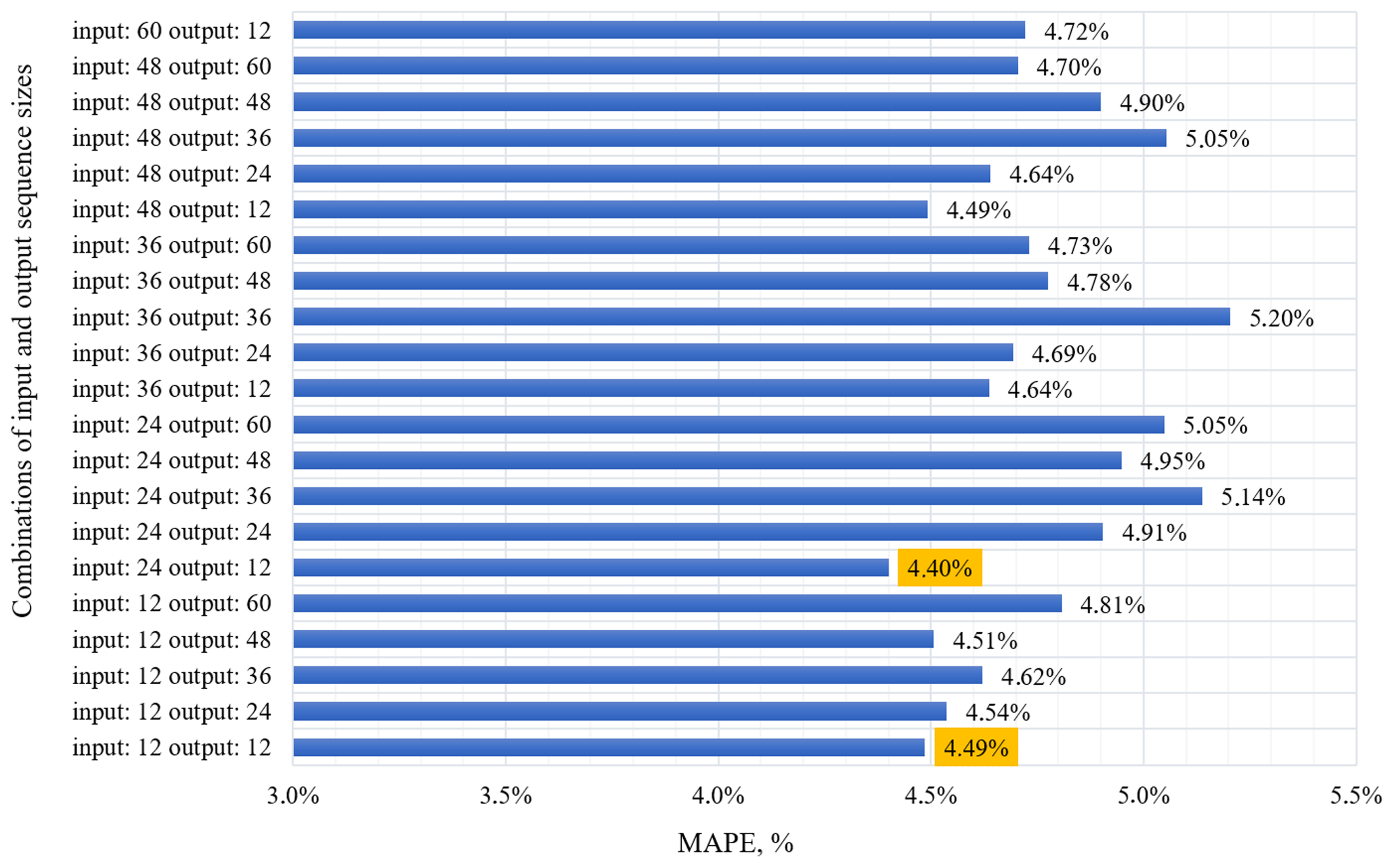
The length of the history sequence refers to the number of previous time steps that the model uses for training and subsequently for predicting the target variable. If the history depth is too small, the model may not have enough information to identify important time patterns; otherwise, training the model may become complex and expensive in terms of computational time. The conducted experiment to find the optimal ratio of history length and forecast horizon took 95,257 s over 20 epochs of model training. In this case, various combinations of input and output data were tried with an assessment of the model quality metrics. In the conducted study, 20 different sets of parameters with history [12, 24, 36, 48] and forecast [12, 24, 36, 48, 60] depths were considered. The figure shows the results of the analysis of the influence of the history depth and the forecast horizon length on the change in the MAPE metric over 20 epochs of model training. In Figure 11 shows the results of the analysis of the influence of the depth of history and the length of the forecasting horizon on the change in the MAPE metric for 20 epochs of model training.

As a result of the experiment, the following conclusions can be made:

(1) With an increase in the length of the input data (history depth), the model training time increases significantly, which is associated with an increase in the dimensions of the data tensor, as a result of which more computing power and time are required to train the model.

(2) With an increase in the length of the forecasting horizon, no stable growth or decrease in the model quality metrics is observed. This may indicate that the dependence between the forecasting horizon and the quality of the model may be non-linear or may change significantly depending on other factors.

(3) Models with fewer input and output data usually show better results in terms of quality and performance metrics.

(4) In certain cases, it was observed that an increase in the length of the output data with a constant length of the input data leads to a deterioration in the quality of the model.

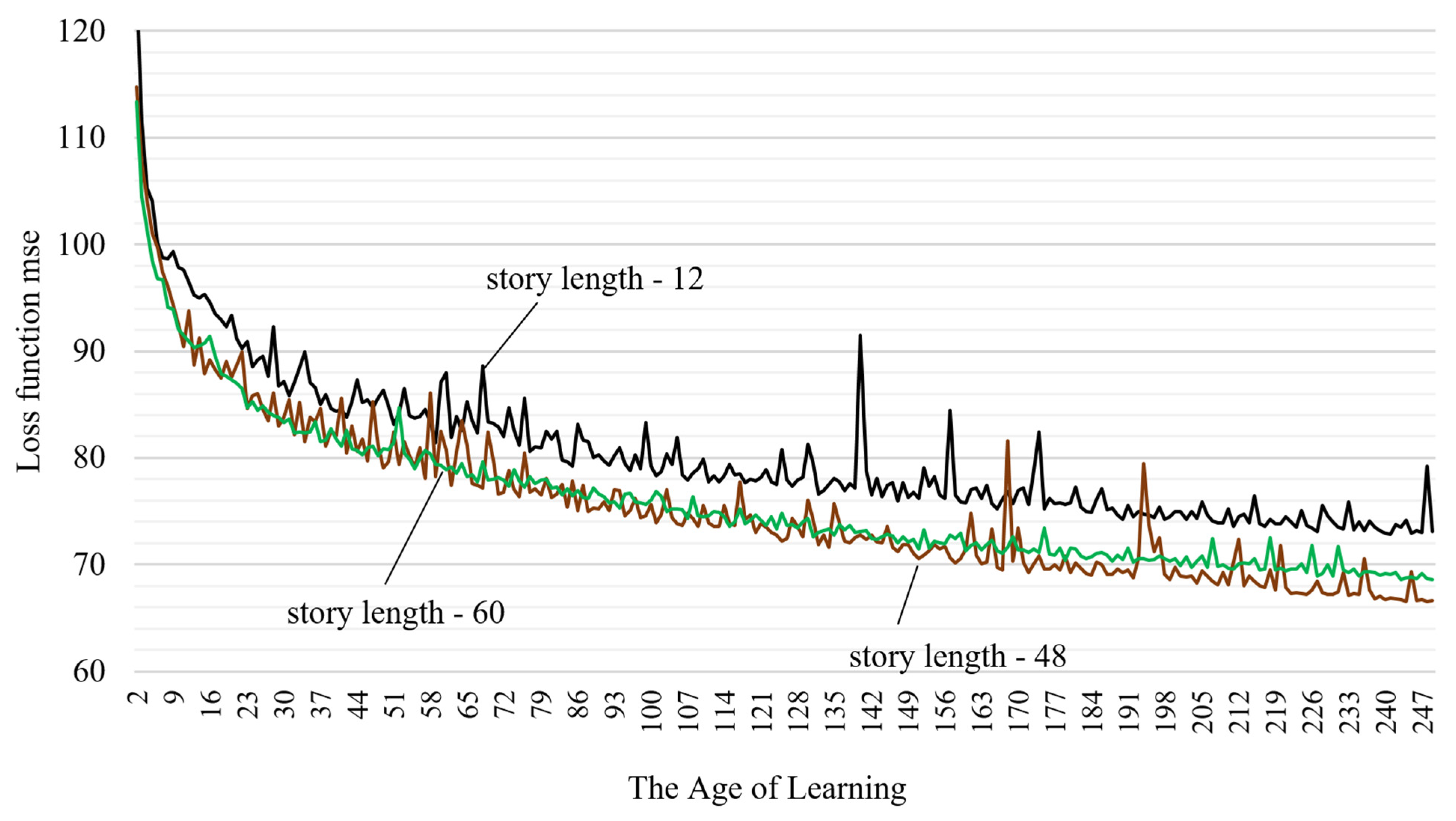
Of particular interest is the change in the loss function during the model training process. To accomplish this, the number of epochs was increased from 20 to 50 and the behavior of the mean square error was assessed for cases with 12, 24, and 60 time steps entering the LSTM model (Figure 12).

Analyzing the results of the experiment, we can conclude that with increasing history depth, a more stable behavior of the mean square error is observed without significant outliers. This indicates better convergence of the model, that is, optimal adjustment of weight coefficients during the training process when receiving a larger amount of input data. A stable decrease in the loss function indicates that the model is more effective in learning on data with 60 time steps compared to 12, but the training time for 200 epochs increased by 50%, and the metric on the MAPE test data was 4.36%.

4.5. LSTM Models Compared with Holt–Winters Model

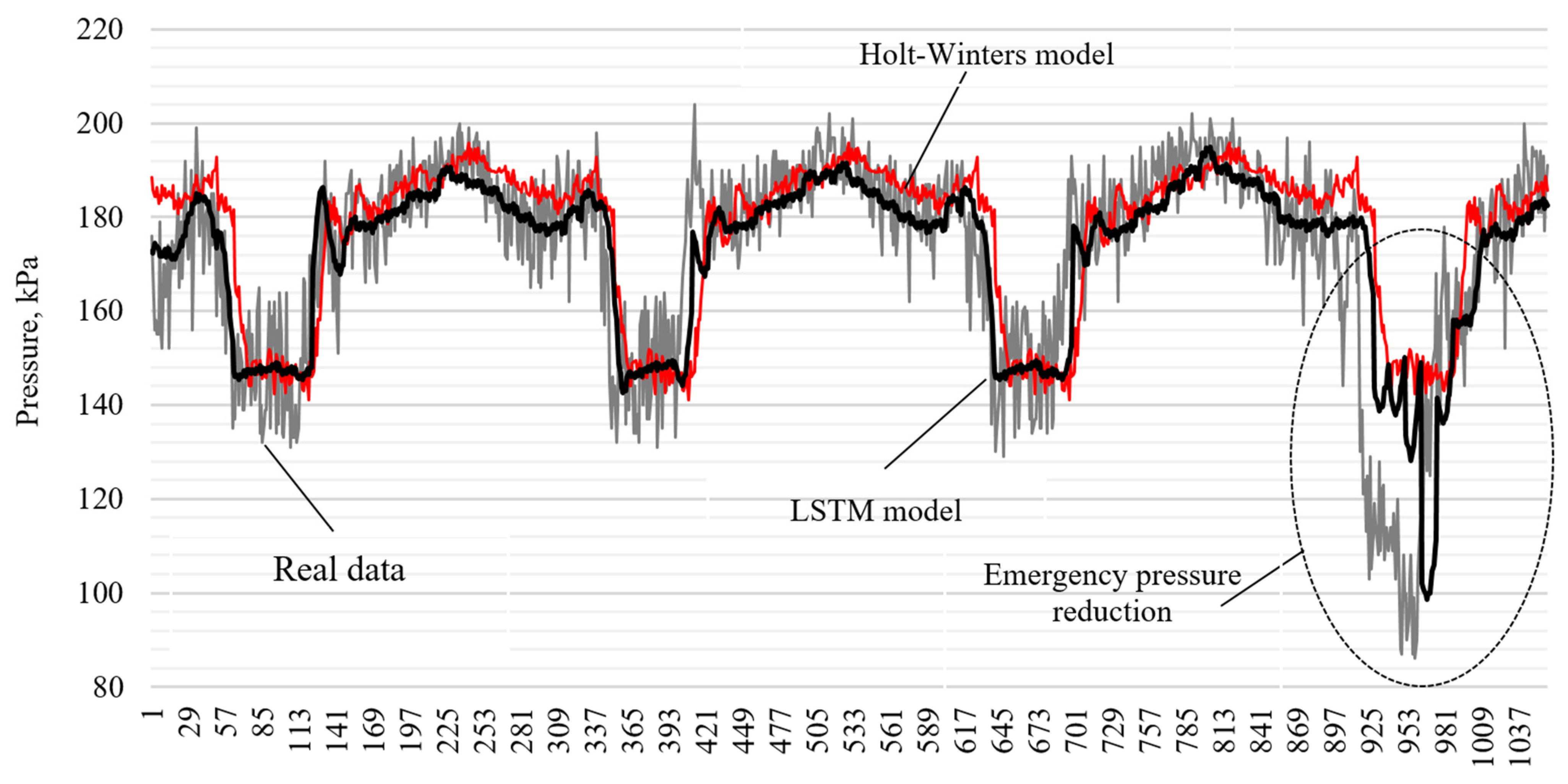
An important step in the study is to demonstrate the advantages of deep learning models. For this purpose, the LSTM model used is compared with the classical simpler Holt–Winters exponential smoothing model [43]. Additive seasonality with a period of 288, which characterizes the daily dynamics with 5 min pressure data, is used as the initial parameters of the exponential smoothing model. A comparison of the quality metrics of the models was carried out on the test data, which included statistics including an emergency pressure drop at the inlet of the booster pumping station (Figure 13). The LSTM model demonstrates a lower forecasting error compared to the Holt–Winters model. The MAPE value for the LSTM model is 4.36%, while the Holt–Winters model has an average absolute percentage error of 6.07%. The MAE metric was 7.35 and 9.86 kPA for the first and second models, respectively. Based on these results, it can be concluded that the LSTM model has a higher quality and provides more accurate data prediction.

It is worth paying special attention to the behavior of the model during an emergency pressure drop. In Figure 13, the LSTM model is built with a forecast for 12 steps (1 h into the future), while the length of the historical data fed to the model was 60 values (5 h of history). It is interesting to note that the recurrent neural network model is able to notice and respond to the falling pressure dynamics, even though in the considered example, the training sample had only one emergency scenario. This indicates high sensitivity and the ability of the model to detect changes in time series, even with limited data at the time of a sudden pressure drop, which does not allow for the implementation of the Holt–Winters model.

5. Conclusions

In the course of this study, an information system for obtaining data on hydraulic pressure in a water supply system was developed. These data were subsequently used to train a long short-term memory (LSTM) model designed to predict pressure in a water supply system and use these forecasts to create preventive methods for responding to accidents. An important stage of the work was to study the influence of the neural network architecture on its performance. It was found that increasing the number of LSTM layers (up to two–three) and using regularization layers (Dropout) contributes to improving the forecast accuracy, while adding additional fully connected layers does not have a significant effect. The optimal configuration of the model includes two LSTM layers, one Dropout layer, and one Dense layer, which provided minimal values of error metrics such as MAPE (4.79%). In addition, a study was conducted on the influence of seasonal factors on forecasting accuracy. It was found that adding parameters such as month, hour, minute, and day type leads to an improvement in the quality of the model and a reduction in forecast errors (MAPE decreased to 4.37%).

The influence of the number of neurons in the LSTM and Dense layers on the model performance was also assessed using the grid search method. Based on the obtained data, the optimal model configuration with 50 neurons in the LSTM layers and 250 neurons in the Dense layer was selected, which provided the best ratio of forecast accuracy and training time. In parallel, the influence of the length of the input and output sequences on the quality of the model was investigated. Increasing the length of the input data (history depth) improved the convergence of the model, but also increased the training time. Models with fewer data demonstrated faster results with comparable forecast accuracy. This confirms that the optimal choice of history depth and forecast length depends on the computing resources and the tasks at hand.

In the final part of the work, the proposed LSTM model was compared with the classical Holt–Winters exponential smoothing model. The results showed that LSTM significantly outperforms the Holt–Winters model both in forecast accuracy (MAPE 4.36 versus 6.07%) and in sensitivity to emergency situations, such as a sharp drop in pressure. Thus, the experiments showed that the use of LSTM models for forecasting pressure in water supply systems significantly improves the accuracy of forecasts, especially when including seasonal factors and optimizing the model architecture. The study is not exhaustive, and other combinations of hyperparameters may be more effective for the task of forecasting water supply network pressure.