Binary Transformer Detectors for Automatic Modulation Detection Under Realistic Radio Frequency Impairment Conditions

Abstract

Automatic modulation classification (AMC) is a core capability for spectrum monitoring, adaptive receivers, and electronic support. Most radio-frequency machine learning (RFML) studies train multi-class classifiers on benchmark datasets that contain a single modulation per recording at baseband. In operational settings, however, the objective is often to detect only a small set of signals of interest, making large multi-class models unnecessarily expensive to train and deploy. In addition, multi-class formulations can increase false-alarm risk due to confusion among non-essential classes and may allocate model capacity inefficiently to distinctions that are irrelevant for the operational objective. This paper investigates an alternative workflow based on targeted binary transformer detectors and evaluates their robustness under practical RF complications. Using the RadioML 2018.01A dataset, we construct binary detection tasks with BPSK as the signal of interest and introduce three increasingly realistic conditions: (i) center-frequency shifts away from baseband, (ii) sampling-rate mismatches via decimation and interpolation, and (iii) multi-signal mixtures where modulations co-occur either in frequency (simultaneous transmissions) or in time (temporal concatenation). The results show that baseband-trained detectors do not generalize to center-frequency-shifted signals, and multi-signal interference can cause complete detection failure unless explicitly modeled during training. We investigate early-exit transformer inference to reduce computation on high-confidence examples, showing it maintains (and occasionally improves) detection performance. We also evaluate inter-modulation transfer learning and intra-modulation adaptation from baseband to mixed- and multi-signal scenarios.

1. Introduction

Automatic signal detection and modulation recognition underpin many commercial, scientific, and defense applications, ranging from adaptive and cognitive radios to spectrum monitoring and electronic support [1,2]. In commercial wireless systems, modulation awareness can support adaptive links that change modulation and coding in response to channel conditions, spectrum access policies, and multi-user interference [3]. In public safety, industrial IoT, and satellite systems, fast recognition of the waveform in an occupied channel can provide situational awareness and facilitate coexistence in congested spectrum [4,5]. In defense and spectrum-surveillance settings, rapid detection of specific emitters enables downstream tasks such as interception, localization, jamming, and prioritization of operator attention [6]. These tasks are often time-critical in dynamic environments where an adversary may rapidly change waveform parameters or hop frequencies. The safety and security of radio frequency (RF) signals have garnered increasing attention, particularly in the context of adversarial environments and intelligent wireless systems. Emerging techniques such as distributed time-modulated arrays and intelligent reflecting surface (IRS)-assisted beamforming have been proposed to enhance physical-layer security and mitigate unauthorized interception. These approaches highlight the growing need for robust and adaptive signal detection frameworks capable of operating under realistic RF conditions and potential security threats [7,8].

To better position this work within the AMC literature, it is important to distinguish between classical and deep learning approaches and their limitations. Classical AMC methods rely on expert-designed features such as higher-order statistics and cyclostationary properties, followed by conventional classifiers. While effective in controlled settings, these approaches require significant domain knowledge and often degrade under realistic RF impairments.

More recently, deep learning approaches—including convolutional neural networks (CNNs), recurrent neural networks (RNNs), and transformer-based models—have demonstrated strong performance by learning directly from raw IQ data. However, most prior work focuses on multi-class classification in idealized conditions, typically assuming single-modulation, baseband-centered signals (e.g., RadioML datasets). These assumptions do not reflect operational environments, where frequency offsets, sampling mismatches, and multi-signal interference are common.

This creates a gap between benchmark-driven AMC research and real-world deployment. In particular, limited attention has been given to task formulations that focus on detecting a specific signal of interest under realistic RF impairments. This work addresses this gap by combining a binary detection framework with explicitly modeled real-world signal conditions.

Classical automatic modulation classification (AMC) relies on expert-designed features extracted from the waveform or its statistics (e.g., higher-order moments and cyclic/cyclostationary features), followed by decision rules or conventional classifiers [9]. While many recent RFML models operate directly on raw IQ samples [10], alternative approaches rely on extracted representations such as constellation or eye diagrams [11,12].

Convolutional and recurrent architectures are widely used in this setting [13,14,15,16,17,18,19,20,21]. Ensemble learning approaches combine multiple weak or moderately performing learners to form a stronger composite network. In RF modulation recognition, such ensembles can improve robustness to noise and channel impairments by aggregating complementary decision boundaries learned by individual models [22,23]. Transformer models have emerged as a strong alternative for modulation analysis [24,25]. Transformers are attractive because self-attention can represent global relationships across an observation window and can emphasize salient waveform regions without being restricted to a local receptive field [26]. This property is particularly relevant for digitally modulated signals whose discriminative structure can span multiple symbol intervals.

Despite strong benchmark results, two gaps commonly arise when transitioning from benchmark-driven RFML to operational deployment. The first gap is data realism. Public benchmarks (including the RadioML family) typically provide short, single-modulation recordings centered at baseband and sampled at a nominal rate with labels provided per recording [27,28]. Field recordings often violate these assumptions. Center-frequency offsets and Doppler introduce linear phase ramps; sampling-rate mismatch (and any subsequent resampling) distorts time-domain structure [29]; and wideband sensing frequently yields mixtures where multiple transmissions co-occur within the same window [2]. Such co-occurrence may be spectral (simultaneous transmissions in adjacent or overlapping bands) or temporal (bursts of different modulations concatenated within a fixed-length capture). Models trained exclusively on idealized baseband single-signal examples can therefore fail unexpectedly when confronted with realistic RF complications.

The second gap is task mismatch. Many RFML studies train a single multi-class model over all available modulations because it is convenient for benchmarking. In practical monitoring systems, however, an operator is often interested in detecting only a small set of signals of interest (SOIs) within a particular band or mission context. Training and deploying a large multi-class model can be unnecessarily expensive, and it can increase false-alarm risk due to label confusion among non-essential classes. A practical alternative is a bank of lightweight binary detectors, one per SOI, each solving a simpler decision problem (SOI versus background). Such detectors can be tailored to the modulations that plausibly co-occur in the target band, can run in parallel across bands and hardware resources, and can be extended incrementally by adding new detectors without retraining an entire multi-class system.

This paper investigates this targeted workflow using transformer-based binary detectors and explicitly evaluates robustness under RF impairments that challenge common AMC assumptions. Using the RadioML 2018.01A dataset, we formulate binary detection tasks with BPSK as the SOI and introduce three increasingly realistic conditions: (i) center-frequency shifts away from baseband via frequency mixing, (ii) sampling-rate mismatch through decimation and interpolation, and (iii) multi-signal mixtures in which modulations co-occur either in frequency (simultaneous transmissions) or in time (temporal concatenation) [30,31]. We also study early-exit transformer inference [32] to reduce computation on high-confidence examples and assess transfer learning between related modulations as a potential pathway for scaling detector training [33]. Beyond aggregate confusion-matrix metrics, we analyze false alarms and missed detections as functions of SNR to identify the operating regimes that dominate the error budget.

BPSK is selected as the signal of interest (SOI) due to its simplicity, ubiquity, and well-understood structure in digital communication systems. As one of the most fundamental modulation schemes, BPSK provides a clean and interpretable baseline for studying detector behavior under controlled conditions. Its constant-envelope, binary phase structure allows the effects of RF impairments—such as frequency offsets, sampling mismatches, and multi-signal interference—to be isolated without additional complexity introduced by higher-order constellations. Moreover, while many AMC studies directly train on benchmark datasets under idealized assumptions, the experimental conditions considered here (e.g., mixed-frequency shifts and multi-signal superposition) are less commonly explored. Beginning with a simple and widely used modulation enables a focused investigation of these effects. Although the results may not directly generalize to all modulation types, the intent is to first establish and validate the proposed framework in a controlled setting, which can then be systematically extended to more complex modulations in future work. Such extensions may require frequency-aware or modulation-aware architectures, incorporation of auxiliary metadata, or specialized feature representations.

Additionally, even within BPSK, variations such as differing symbol (baud) rates introduce further complexity that is not explicitly modeled in this study, highlighting an additional limitation and direction for future investigation. Finally, while additional modulation classes could be incorporated, a small increase in class diversity would still be insufficient to support broad generalization, reinforcing the need for a more systematic expansion of the experimental space in future work.

The main contributions of this study are: (a) A binary transformer detection formulation for AMC that targets a specific SOI (BPSK) against a background of other modulation types, enabling a modular “bank of detectors” deployment; (b) A controlled robustness study under practical RF complications: frequency mixing (center-frequency shifts), sampling-rate changes (decimation/interpolation), and multi-signal mixtures (frequency- and time-domain co-occurrence); (c) A time-domain perspective on why self-attention is a natural fit for IQ-based detection, including intuition for frequency-shifted and multi-signal settings; (d) An early-exit transformer inference study, showing that high-confidence (high-SNR) samples can exit early to reduce computation while preserving detection performance; (e) An evaluation of transfer learning across related modulation schemes, examining the limitations inherent in a detector-style formulation and extending the framework to intra-modulation tasks, such as adapting a baseband model from mixed-signal scenarios to multi-signal environments [30,33,34].

2. Motivation and Problem Formulation

In a typical wideband RF processing chain, captured IQ samples are often analyzed using time-frequency methods such as the short-time Fourier transform (STFT). The frequency resolution of an $N_{\mathrm{FFT}}$-point FFT is $\Delta f=f_s/N_{\mathrm{FFT}}$, where $f_s$ is the sampling rate. Increasing $N_{\mathrm{FFT}}$ improves frequency resolution but increases computational cost, which is critical for real-time monitoring.

Depending on the bandwidth per frequency bin and the spectral occupancy, a bin (or a small group of adjacent bins) may contain multiple bursts with different modulations. In some bands, regulations or operational knowledge may indicate that only a small set of modulations is plausible. In such settings, it can be more efficient to deploy a bank of lightweight binary detectors (one per SOI) instead of a single large multi-class model. Each detector focuses on discriminating the SOI from background signals likely to co-occur in that band.

In practice, wideband monitoring commonly combines signal processing and ML: an initial detector (e.g., energy detection [35] or image/object detection on spectrograms [36,37,38]) localizes candidate emissions; the isolated emission is then passed to a modulation classifier. The experiments in this paper focus on the classifier stage and study how realistic RF complications affect a transformer-based binary detector.

3. Mathematical Justification for Attention on Time-Domain IQ Signals

Before employing self-attention mechanisms for RF signal detection and modulation analysis, we first consider three increasingly realistic scenarios: (i) a single baseband signal, (ii) a single signal with a center-frequency offset, and (iii) the superposition of multiple signals at distinct center frequencies.

3.1. Setup and Notation (Exact)

Remark on interpretation of equations: In this section, we distinguish between exact identities, approximations, and intuitive interpretations. Exact expressions follow directly from algebraic definitions of IQ signals and attention mechanisms. Approximate relations rely on assumptions such as limited amplitude variation, structure-preserving projections, and phase-dominant behavior. For clarity, each key equation is labeled accordingly, and the conditions under which approximations hold are stated explicitly.

Let the discrete-time complex baseband signal be

$$x\left[n\right]=I\left[n\right]+jQ\left[n\right]=a\left[n\right]e^{j\varphi \left[n\right]},n=1,\dots ,T.$$

(1)

This representation is exact by definition of the complex baseband signal, where $a\left[n\right]\ge 0$ and $\varphi \left[n\right]\in \mathbb{R}$.

We define a real-valued embedding

$${\mathbf{x}}_n=g(I\left[n\right],Q\left[n\right])\in {\mathbb{R}}^d.$$

(2)

This is exact once the embedding function $g(·)$ is specified (e.g., linear or nonlinear projection).

3.2. Self-Attention (Exact)

Queries, keys, and values are computed as

$${\mathbf{q}}_n={\mathbf{x}}_n{W}_Q,{\mathbf{k}}_m={\mathbf{x}}_m{W}_K,{\mathbf{v}}_m={\mathbf{x}}_m{W}_V.$$

(3)

Attention weights are

$${\alpha }_{n,m}={\displaystyle \frac{\exp \left(\langle {\mathbf{q}}_n,{\mathbf{k}}_m\rangle /\sqrt{d}\right)}{{\sum }_{\ell =1}^T\exp \left(\langle {\mathbf{q}}_n,{\mathbf{k}}_{\ell }\rangle /\sqrt{d}\right)}}.$$

(4)

The output is

$${\mathbf{z}}_n={\displaystyle \sum _{m=1}^T}{\alpha }_{n,m}{\mathbf{v}}_m.$$

(5)

All equations in this subsection are exact.

3.3. Step-by-Step Expansion of Attention (Exact)

For clarity, consider a 2D embedding:

$${\mathbf{x}}_n=\left[\begin{array}{c}I\left[n\right]\\ Q\left[n\right]\end{array}\right].$$

(6)

Then each query component is

$$q_n^{\left(r\right)}=I\left[n\right]w_{1r}^Q+Q\left[n\right]w_{2r}^Q,$$

(7)

and similarly for keys:

$$k_m^{\left(r\right)}=I\left[m\right]w_{1r}^K+Q\left[m\right]w_{2r}^K.$$

(8)

The dot product becomes

$$\langle {\mathbf{q}}_n,{\mathbf{k}}_m\rangle ={\displaystyle \sum _{r=1}^d}{q}_n^{\left(r\right)}{k}_m^{\left(r\right)}.$$

(9)

Substituting:

$$\begin{array}{cc}\hfill q_n^{\left(r\right)}{k}_m^{\left(r\right)}& =(I\left[n\right]w_{1r}^Q+Q\left[n\right]w_{2r}^Q)(I\left[m\right]w_{1r}^K+Q\left[m\right]w_{2r}^K)\hfill \end{array}$$

(10)

$$\begin{array}{cc}\hfill & =I\left[n\right]I\left[m\right]w_{1r}^Q{w}_{1r}^K+I\left[n\right]Q\left[m\right]w_{1r}^Q{w}_{2r}^K\hfill \end{array}$$

(11)

$$\begin{array}{cc}\hfill & +Q\left[n\right]I\left[m\right]w_{2r}^Q{w}_{1r}^K+Q\left[n\right]Q\left[m\right]w_{2r}^Q{w}_{2r}^K.\hfill \end{array}$$

(12)

Summing over r:

$$\langle {\mathbf{q}}_n,{\mathbf{k}}_m\rangle =AI\left[n\right]I\left[m\right]+BI\left[n\right]Q\left[m\right]+CQ\left[n\right]I\left[m\right]+DQ\left[n\right]Q\left[m\right],$$

(13)

where $A,B,C,D$ are learned coefficients. This expression is exact and does not assume any constraints on signal amplitude or phase.

3.4. Connection to Complex Correlation (Exact Identity)

Consider the complex product

$$x\left[n\right]x^{*}\left[m\right]=(I\left[n\right]+jQ\left[n\right])(I\left[m\right]-jQ\left[m\right]).$$

(14)

Expanding:

$$x\left[n\right]x^{*}\left[m\right]=I\left[n\right]I\left[m\right]+Q\left[n\right]Q\left[m\right]+j\left(Q\left[n\right]I\left[m\right]-I\left[n\right]Q\left[m\right]\right).$$

(15)

Thus,

$$\mathrm{Re}\left(x\left[n\right]x^{*}\left[m\right]\right)=I\left[n\right]I\left[m\right]+Q\left[n\right]Q\left[m\right].$$

(16)

This identity is exact.

3.5. Approximation to Phase Similarity (Approximate)

If the learned projections approximately satisfy the following structural assumptions:

• symmetric weighting of I/Q terms,
• suppression of cross terms $I\left[n\right]Q\left[m\right],Q\left[n\right]I\left[m\right]$,

then the attention score can be approximated as

$$\langle {\mathbf{q}}_n,{\mathbf{k}}_m\rangle \approx \gamma \left(I\left[n\right]I\left[m\right]+Q\left[n\right]Q\left[m\right]\right),$$

(17)

for some learned scalar $\gamma$.

Using the exact identity above,

$$\langle {\mathbf{q}}_n,{\mathbf{k}}_m\rangle \approx \gamma \mathrm{Re}\left(x\left[n\right]x^{*}\left[m\right]\right).$$

(18)

If additionally $a\left[n\right]\approx a\left[m\right]\approx 1$ (unit or slowly varying envelope),

$$\mathrm{Re}\left(x\left[n\right]x^{*}\left[m\right]\right)=a\left[n\right]a\left[m\right]\cos (\varphi \left[n\right]-\varphi \left[m\right])\approx \cos (\varphi \left[n\right]-\varphi \left[m\right]).$$

(19)

Therefore,

$$\langle {\mathbf{q}}_n,{\mathbf{k}}_m\rangle \approx \gamma \cos (\varphi \left[n\right]-\varphi \left[m\right]).$$

(20)

This approximation holds when amplitude variation is limited and learned projections align with the real part of the complex inner product.

3.6. Frequency Offset Case (Exact + Approximate)

Let the observed signal be

$$y\left[n\right]=x\left[n\right]e^{j\omega n},\omega =2\pi \Delta f/f_s.$$

(21)

This is exact.

Then

$$\begin{array}{cc}\hfill y\left[n\right]y^{*}\left[m\right]& =x\left[n\right]x^{*}\left[m\right]e^{j\omega (n-m)}\hfill \end{array}$$

(22)

$$\begin{array}{cc}\hfill & =a\left[n\right]a\left[m\right]e^{j\left(\varphi \right[n]-\varphi [m]+\omega (n-m\left)\right)}.\hfill \end{array}$$

(23)

Taking real part:

$$\mathrm{Re}\left(y\left[n\right]y^{*}\left[m\right]\right)=a\left[n\right]a\left[m\right]\cos (\varphi \left[n\right]-\varphi \left[m\right]+\omega (n-m)).$$

(24)

If the same projection assumptions as above hold, then

$$\langle {\mathbf{q}}_n,{\mathbf{k}}_m\rangle \approx \gamma \cos (\varphi \left[n\right]-\varphi \left[m\right]+\omega (n-m)).$$

(25)

This approximation assumes:

• projections preserve phase relationships,
• amplitude variation is limited or absorbed into scaling.

3.7. Interpretation (Intuitive)

The attention mechanism computes weighted interactions between all time pairs $(n,m)$, where the weights depend on learned mixtures of $I/Q$ cross-products. Under mild conditions, this reduces to measuring phase coherence across time, modulated by relative time differences $(n-m)$ in the presence of frequency offsets.

Thus, self-attention behaves as a learned, data-driven generalization of complex correlation, enabling robustness to frequency translation while operating directly on time-domain IQ samples.

3.8. Multi-Signal Superposition at Distinct Center Frequencies

Finally, consider a realistic scenario in which two signals coexist within the same observation window:

$$y\left[n\right]=x_1\left[n\right]e^{j2\pi f_{1}n/f_s}+x_2\left[n\right]e^{j2\pi f_{2}n/f_s},$$

(26)

where $f_1\ne f_2$.

Each component can be written in amplitude-phase form:

$$x_i\left[n\right]=a_i\left[n\right]e^{j{\varphi }_i\left[n\right]},i\in \{1,2\}.$$

(27)

Thus,

$$y\left[n\right]=a_1\left[n\right]e^{j({\varphi }_1\left[n\right]+2\pi f_{1}n/f_s)}+a_2\left[n\right]e^{j({\varphi }_2\left[n\right]+2\pi f_{2}n/f_s)}.$$

(28)

The complex correlation between samples n and m is:

$$y\left[n\right]y^{*}\left[m\right].$$

(29)

Expanding:

$$\begin{array}{cc}\hfill y\left[n\right]y^{*}\left[m\right]& ={\displaystyle \sum _{i=1}^2}{a}_i\left[n\right]a_i\left[m\right]e^{j({\varphi }_i\left[n\right]-{\varphi }_i\left[m\right]+2\pi f_i(n-m)/f_s)}\hfill \end{array}$$

(30)

$$\begin{array}{cc}\hfill & +\sum _{i\ne j}{a}_i\left[n\right]a_j\left[m\right]e^{j({\varphi }_i\left[n\right]-{\varphi }_j\left[m\right]+2\pi (f_i-f_j)(n-m)/f_s)}.\hfill \end{array}$$

(31)

The first summation corresponds to within-signal terms, while the second corresponds to cross terms between distinct signals.

Taking the real part:

$$\begin{array}{cc}\hfill \mathrm{Re}\left(y\left[n\right]y^{*}\left[m\right]\right)& ={\displaystyle \sum _{i=1}^2}{a}_i\left[n\right]a_i\left[m\right]\cos ({\varphi }_i\left[n\right]-{\varphi }_i\left[m\right]+2\pi f_i(n-m)/f_s)\hfill \end{array}$$

(32)

$$\begin{array}{cc}\hfill & +\sum _{i\ne j}{a}_i\left[n\right]a_j\left[m\right]\cos ({\varphi }_i\left[n\right]-{\varphi }_j\left[m\right]+2\pi (f_i-f_j)(n-m)/f_s).\hfill \end{array}$$

(33)

The cross terms contain oscillatory factors:

$$\cos \left(2\pi (f_i-f_j)(n-m)/f_s\right),$$

(34)

which vary rapidly when $f_i\ne f_j$.

(Approximation) When the frequency separation is sufficiently large, these oscillatory cross terms average out (decorrelate) across $(n,m)$ and are suppressed after softmax normalization. Under this condition,

$$\langle {\mathbf{q}}_n,{\mathbf{k}}_m\rangle \approx {\displaystyle \sum _{i=1}^2}\langle {\mathbf{q}}_n^{\left(i\right)},{\mathbf{k}}_m^{\left(i\right)}\rangle .$$

(35)

Consequently, the attention weights decompose approximately into signal-specific components:

$${\alpha }_{n,m}\approx {\alpha }_{n,m}^{\left(1\right)}+{\alpha }_{n,m}^{\left(2\right)}.$$

(36)

This approximation holds when frequency separation is sufficient to decorrelate cross terms and when learned projections preserve phase-coherent structure.

Multi-head attention further reinforces this behavior by allowing different heads to specialize in distinct phase-coherent structures. Each head effectively acts as a learned, soft matched filter that selectively attends to one signal while suppressing interference from others, without requiring explicit frequency-domain separation.

4. Study Data Preparation

4.1. RadioML 2018.01A Dataset

RadioML 2018.01A contains 24 modulation classes with $\mathrm{106,496}$ samples per class, totaling $\mathrm{2,555,904}$ IQ recordings $(24\times \mathrm{106,496})$ [31]. Each recording contains $T=1024$ complex samples represented by two real-valued streams (in-phase and quadrature). The dataset provides labeled SNR values ranging from $-20$ dB to 30 dB in 2 dB increments.

For reliable evaluation across SNR, the dataset is not split using a purely random shuffle. Instead, training/validation/test splits are constructed to maintain a balanced representation across all SNR values. An 80–10–10 split is used for training, validation, and testing, respectively. Due to dataset size and the number of experiments in this paper, approximately a quarter of the available data is used.

For validation and testing, there are 100 samples per SNR (26 distinct SNR values from $-20$ dB to 30 dB) per class, i.e., 2600 samples per class. For the binary setting with one positive class (BPSK) and 23 negative classes, this yields 2600 positive samples and $\mathrm{59,800}$ negative samples per split.

For training, there are 1000 samples per SNR (26 distinct SNR values), i.e., $\mathrm{26,000}$ samples per class. In the same binary setting, this corresponds to $\mathrm{26,000}$ positive samples and $\mathrm{598,000}$ negative samples.

4.2. Mixed-Frequency (Center-Frequency Shifted) Data

To model recordings where the SOI is not centered at baseband, each IQ sample is frequency shifted by multiplying it by a complex exponential. Given a discrete-time complex signal $x\left[n\right]$, a frequency shift of $\Delta f$ (Hz) is:

$$y\left[n\right]=x\left[n\right]e^{-j2\pi \Delta f{\displaystyle \frac{n}{f_s}}},$$

(37)

where $f_s$ is the sampling frequency. If the offset is expressed in normalized form,

$$ϵ={\displaystyle \frac{\Delta f}{f_s}}.$$

(38)

The dataset does not provide $f_s$ explicitly; therefore, the experiments use a normalized relative frequency offset parameter $ϵ$, uniformly sampled in the range $[-200,200]$.

4.3. Multi-Signal Mixture Data

Operational RF captures frequently contain multiple simultaneous transmissions within the same observation window. To emulate this complexity, we generate two-signal mixtures by adding a discriminator modulation to the anchor signal.

BPSK is selected as the anchor (SOI), and QPSK is used as the discriminator. Let $x_{\mathrm{BPSK}}\left[n\right]=I_{\mathrm{BPSK}}\left[n\right]+j{Q}_{\mathrm{BPSK}}\left[n\right]$ denote the anchor signal and $x_{\mathrm{QPSK}}\left[n\right]=I_{\mathrm{QPSK}}\left[n\right]+j{Q}_{\mathrm{QPSK}}\left[n\right]$ denote the inserted signal. The mixed recording is:

$$x_{\mathrm{mix}}\left[n\right]=x_{\mathrm{BPSK}}\left[n\right]+x_{\mathrm{QPSK}}\left[n\right].$$

(39)

Equivalently, in terms of the I/Q components:

$$I_{\mathrm{mix}}\left[n\right]=I_{\mathrm{BPSK}}\left[n\right]+I_{\mathrm{QPSK}}\left[n\right],$$

(40)

$$Q_{\mathrm{mix}}\left[n\right]=Q_{\mathrm{BPSK}}\left[n\right]+Q_{\mathrm{QPSK}}\left[n\right].$$

(41)

For interpretability, mixtures are generated by combining signals at the same nominal SNR value.

QPSK is selected as the interfering (discriminator) signal due to its structural similarity to BPSK and its prevalence in practical communication systems. Both modulations share constant-envelope properties and phase-based encoding, with QPSK effectively extending BPSK by introducing additional phase states. This makes QPSK a challenging and realistic interferer, as its superposition with BPSK can produce composite signal characteristics that are difficult to distinguish. By choosing QPSK, the experiment intentionally evaluates the detector under a hard discrimination scenario, where interference arises from a modulation with closely related statistical and spectral properties rather than from a fundamentally different signal type.

While many alternative modulation types (e.g., higher-order PSK such as 8PSK, or analog schemes such as FM) could also be used to construct interference scenarios, this study intentionally narrows its scope to a representative and controlled case. The goal is not to exhaustively evaluate all possible modulation pairings—which would be combinatorially large—but to isolate the effect of structured, realistic interference under well-understood conditions. Higher-order PSK introduces additional phase states that increase constellation complexity, while analog modulations such as FM differ fundamentally in their signal characteristics, potentially confounding the interpretation of results. By focusing on BPSK–QPSK interactions, the study captures a meaningful and challenging interference case while maintaining experimental clarity and reproducibility. This controlled setup provides a foundation that can be systematically extended to more diverse modulation combinations in future work.

4.4. Time-Domain Contamination Data

To isolate the effect of temporal (rather than spectral) interference, a separate experiment concatenates two modulations in time at baseband. BPSK is placed at the beginning of the 1024-sample window and QPSK fills the remainder. The proportion of the window occupied by BPSK is swept in 10% increments to study how detection metrics change as the SOI becomes more or less visible.

5. Research Methodology

5.1. Binary Detection Formulation

Each input is a time sequence with $T=1024$ samples and two channels (I and Q). The primary task is formulated as a binary detection problem with BPSK as the positive class ($y=1$) and all remaining modulations as negatives ($y=0$), unless otherwise specified for multi-signal experiments.

The data is then passed into a binary transformer detector which produces a scalar logit output $z=f_{\theta }\left(X\right)$. The probability is obtained using the sigmoid function $\sigma \left(z\right)$.

5.2. Loss Function and Optimization

Because the dataset is strongly imbalanced (one positive modulation versus many negatives in the first two experiments, and multiple positive mixture classes in the later experiments), training uses a weighted binary cross-entropy loss with logits (BCEWithLogitsLoss). The loss is:

$$\mathcal{L}(y,z)=-\left[w_{+}y\log \left(\sigma \left(z\right)\right)+(1-y)\log (1-\sigma \left(z\right))\right],$$

(42)

where $w_{+}$ is a positive-class weighting term (pos_weight), which is selected via Optuna as part of the hyperparameter optimization process rather than fixed a priori. Training is performed using the Adam optimizer with mini-batch gradient descent. Each batch consists of tuples $(X,y,Z)$, where X is the I/Q sequence, y is the binary label, and Z is the associated SNR value. The SNR term is employed for analysis but was not used directly by the loss. The batch size was 32.

5.3. Hyperparameter Tuning with OPTUNA

Transformer training is computationally expensive, making exhaustive grid search impractical. Hyperparameters are tuned using Optuna, which prioritizes promising regions of the search space based on previous trials. The details of the parameters and their search ranges are provided in

Table 1. Transformer hyperparameter and optimization search space (Optuna).

Parameter	Search Range/Choices
$d_{\mathrm{model}}$	{32, 64}
$n_{\mathrm{head}}$	{4, 8}
Number of Layers	{2, 4}
${\dim }_{\mathrm{ff}}$	{64, 128}
Learning rate ($lr$)	$[{10}^{-4},{10}^{-3}]$ (log-uniform)
Data and training parameters
pos_weight	Log-uniform range around class imbalance ratio (∼1–30)
Decision threshold (t)	Selected via validation PR curve (maximize F1-score)
Dataset usage	Stratified subset (∼25% of full dataset)

.

Each Optuna trial samples a transformer configuration, performs a short training run, and evaluates performance on the validation set. Due to class imbalance, trials are ranked using the area under the precision–recall curve (PR-AUC). After selecting the best configuration, a final model is trained for 10 epochs. In addition to architectural parameters, Optuna is also used to tune data-related and decision parameters, including class weighting (pos_weight) and classification threshold selection (see Section 5.4).

5.4. Data Methodology and Hyperparameter Transparency (Optuna-Controlled)

To ensure reproducibility and clarity, all key data-handling and model-selection parameters are explicitly defined and jointly optimized within a unified validation framework.

Positive class weighting (pos_weight): Due to strong class imbalance (one positive modulation versus multiple negatives), the positive-class weighting term in the binary cross-entropy loss is not fixed heuristically. Instead, pos_weight is treated as a hyperparameter and optimized using Optuna. The parameter is sampled over a logarithmic range centered around the empirical class imbalance ratio (approximately 30:1), and selected based on validation performance (PR-AUC). This allows the model to balance false positives and false negatives adaptively rather than relying on a fixed theoretical ratio.

Dataset usage (subsampling rationale): The RadioML 2018.01A dataset is large, and this study evaluates multiple experimental conditions (baseband, mixed-frequency, multi-signal, resampling, and transfer learning). To maintain computational feasibility, approximately a quarter of the total dataset is used. Subsets are selected in a stratified manner to preserve class and SNR distributions, ensuring that statistical properties of the full dataset are retained.

Decision threshold selection: The classification threshold is not fixed (e.g., at 0.5). Instead, it is determined using the validation set by computing the precision–recall curve and selecting the threshold that maximizes the F1-score. This threshold is then fixed and applied to the test set, ensuring no data leakage. This procedure enables the model to operate at an optimal precision–recall trade-off, which is particularly important under class imbalance and varying SNR conditions.

Unified optimization perspective: Optuna is used to jointly optimize architectural parameters, class imbalance weighting, and decision threshold selection within a single validation-driven framework. This ensures that all reported performance metrics correspond to a consistent and reproducible configuration, rather than independently chosen design decisions.

5.5. Decision Threshold and Performance Metrics

After training, the model outputs probability scores p on the validation set. A hard prediction $\widehat{y}$ is obtained using a decision threshold t:

$$\widehat{y}=\left\{\begin{array}{cc}1\hfill & p\ge t,\hfill \\ 0\hfill & p<t.\hfill \end{array}\right.$$

(43)

Rather than using a fixed threshold (e.g., $t=0.5$), t is selected from the validation precision–recall curve by maximizing the F1-score. This threshold selection is integrated into the Optuna optimization loop to ensure consistency between model training and operating point selection. Final performance is evaluated using the confusion matrix metrics—true negatives (TN), false positives (FP), false negatives (FN), and true positives (TP). From these, specificity, sensitivity, precision, recall, F1-score, and balanced accuracy are computed and reported. In addition, FP and FN rates are analyzed as a function of SNR.

6. Results and Analysis

6.1. Experiment 1: Baseband Training and Evaluation

The first experiment trains and tests a BPSK detector on the original baseband dataset.

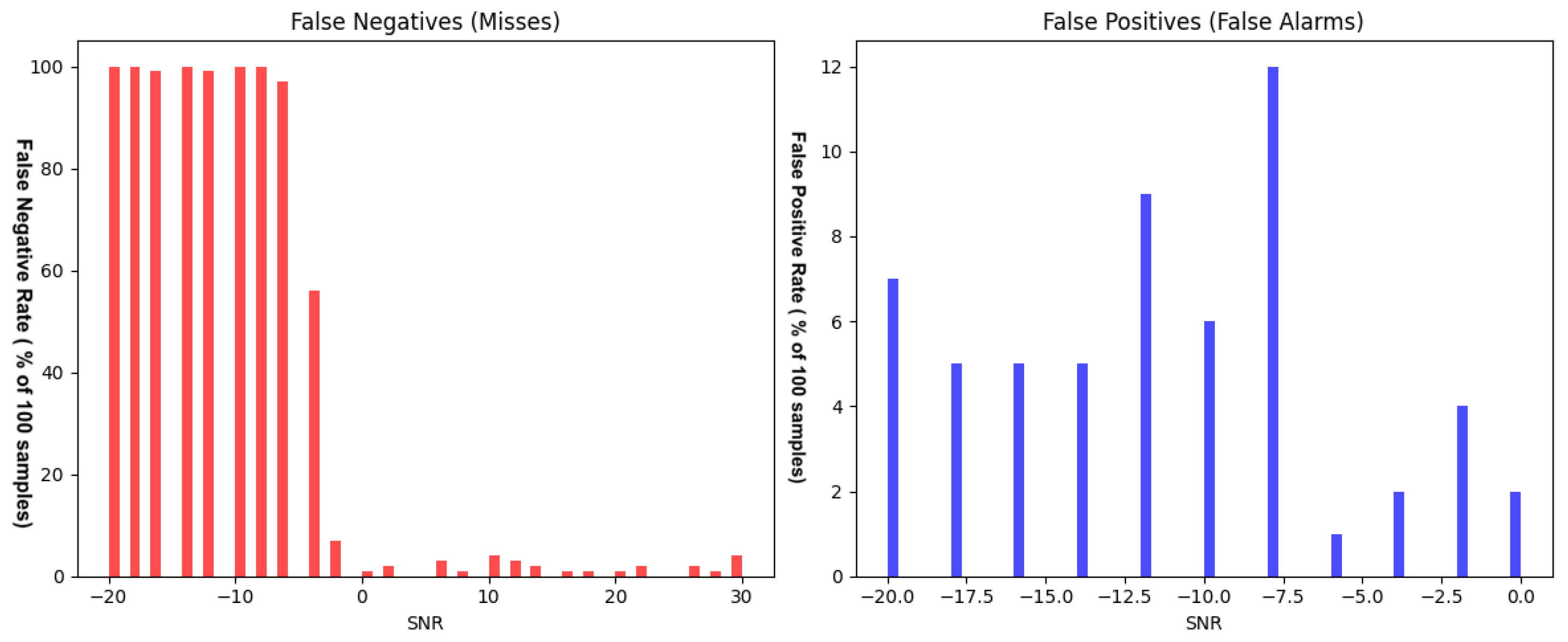
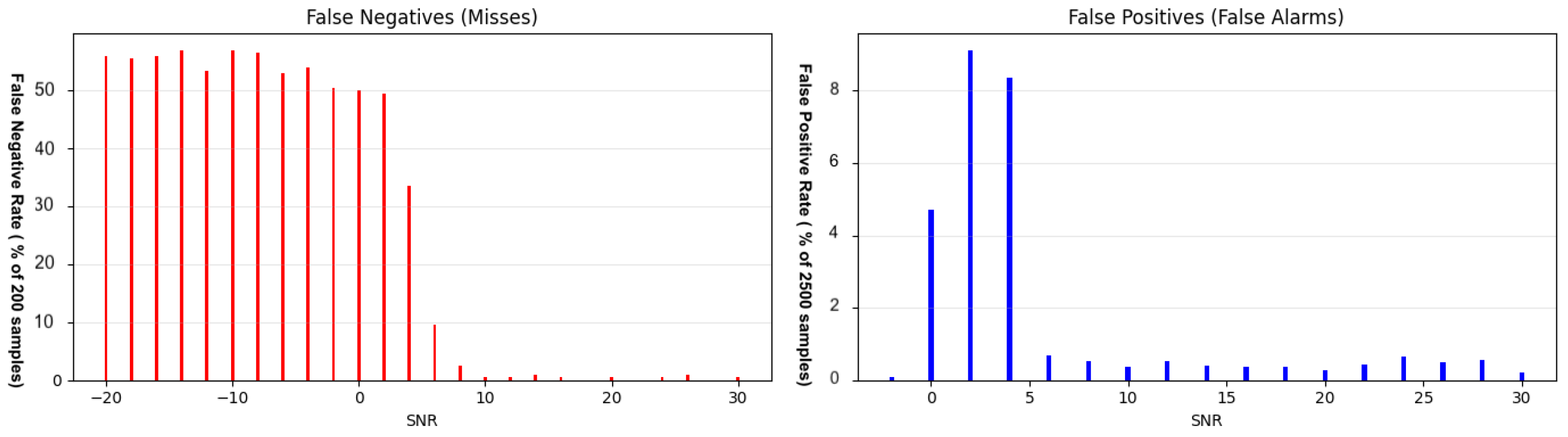
Figure 1 shows that most false negatives occur at low SNR (approximately $-20$ dB to 0 dB), where the SOI is heavily masked by noise. False positives also concentrate in this low-SNR regime.

6.1.1. Generalization to Mixed-Frequency Data

A key question is whether a detector trained only on baseband signals generalizes to signals with a nonzero center-frequency offset.

Table 2. Binary confusion matrix values and derived performance metrics across training and testing scenarios. All values, including derived metrics, are reported as percentages (%). Sensitivity and Recall are equivalent but both are shown for completeness.

Scenario	TN (%)	FP (%)	FN (%)	TP (%)	Spec. (%)	Sens. (%)	Prec. (%)	Recall (%)	F1 (%)	Bal. Acc. (%)
Baseband Train/Test	95.74	0.09	1.42	2.75	99.90	65.92	96.73	65.92	78.56	82.91
Baseband Train, Mixed Test	95.76	0.08	4.16	0.01	99.92	0.27	12.96	0.27	0.53	50.10
Baseband Train/Test, Upsampled (×2)	91.41	4.42	1.57	2.60	95.39	62.32	36.98	62.32	46.18	78.86
Baseband Train/Test, Downsampled (×1/3)	90.28	5.56	1.59	2.57	94.19	61.72	31.65	61.72	41.62	77.96
Baseband Train/Test, Downsampled (×1/2)	90.63	5.21	1.71	2.46	94.57	58.92	32.06	58.92	41.39	76.74
Baseband Train/Test, Downsampled (×1/4)	91.25	4.58	2.11	2.06	95.22	49.35	30.98	49.35	38.05	72.28
Baseband Train/Test, Early Exit	95.80	0.03	1.35	2.82	99.97	67.61	98.93	67.61	80.70	83.79
Mixed Train/Test	95.68	0.16	2.08	2.09	99.84	50.15	93.08	50.15	64.93	74.99
Mixed Train/Test, Upsampled (×2)	95.17	0.66	4.12	0.05	99.31	1.19	7.01	1.19	1.99	50.25
Mixed Train/Test, Decimated (×1/2)	92.43	3.40	2.84	1.33	96.45	31.83	28.04	31.83	29.80	64.14
Mixed Train/Test, Upsampled (×3)	95.83	0.00	4.17	0.00	100.00	0.00	0.00	0.00	0.00	50.00
Mixed Train/Test, Decimated (×1/4)	86.47	9.37	3.61	0.55	90.22	13.31	5.59	13.31	7.92	51.77
Mixed Train/Test, Early Exit	95.79	0.05	1.43	2.74	99.95	65.71	98.27	65.71	78.80	82.83
Multi-Signal (2-Class) Train/Test	90.92	1.08	2.15	5.85	98.83	73.12	84.41	73.12	78.36	85.98
Multi-Signal (3-Class) Train/Test	91.18	1.13	3.41	4.28	98.78	55.62	79.15	55.62	65.33	77.20
Transfer Learning, Early Exit (BPSK→QPSK)	14.15	81.68	0.05	4.11	14.76	98.70	4.80	98.70	9.15	56.73
Transfer Learning, Last Two Layers (BPSK→QPSK)	1.62	23.98	71.85	2.55	6.31	3.43	9.62	3.43	5.19	4.87
Transfer Learning, Early Exit (Baseband→Mixed BPSK)	38.12	57.72	0.65	3.51	39.76	84.30	5.74	84.30	10.74	62.03
Transfer Learning, Last Two Layers (Baseband→Mixed BPSK)	95.00	0.80	2.33	1.88	99.17	44.61	70.20	44.61	54.83	71.89
Transfer Learning, Early Exit (Mixed BPSK→Multi-Signal)	86.58	5.42	2.61	5.39	94.11	67.37	49.86	67.37	57.32	80.74
Transfer Learning, Last Two Layers (Mixed BPSK→Multi-Signal)	91.16	0.84	1.98	6.02	99.08	75.27	87.70	75.27	81.01	87.18

(row “Baseband Train, Mixed Test”) shows a large degradation: FN increases to 4.16% of all samples and TP collapses to 0.01%. The sensitivity drops from 65.9% to 0.27%. In other words, a baseband-trained detector is not robust to center-frequency shifts and must be retrained (or otherwise adapted) for mixed-frequency operation.

6.1.2. Sampling-Rate Mismatch

Sampling-rate mismatch is modeled via resampling. Table 2 shows that upsampling ($\times 2$) reduces TP from 2.75% to 2.60% and increases FN from 1.42% to 1.57%. Sensitivity degrades from 65.92% at baseband to 62.32% with upsampling and to 61.72%, 58.92%, and 49.35% under downsampling by 1/3, 1/2, and 1/4. Downsampling also degrades performance, with larger penalties as the resampling ratio deviates further from 1.

6.2. Experiment 2: Mixed-Frequency Training and Robustness

Because Experiment 1 indicates poor generalization to frequency-shifted signals, Experiment 2 trains and tests the detector on mixed-frequency data. The false positive and false negative rates are shown in Figure 2.

Compared to baseband training, mixed-frequency training slightly reduces the overall TP count (2.09% versus 2.75% in Table 2, which is consistent with the added complexity introduced by frequency offsets).

As derived in Section 3, the attention mechanism can learn phase relationships directly from time-domain IQ samples, enabling adaptation to non-baseband conditions. This suggests that performance can be recovered even under more complex signal scenarios. The experimental results confirm this behavior, demonstrating that the model learns the underlying structure as predicted by the formulation.

6.2.1. Sampling-Rate Mismatch in Mixed-Frequency Data

Table 2 shows a notable asymmetry for mixed-frequency resampling: upsampling ($\times 2$) yields a TP of only 0.05%, whereas decimation ($\times 1/2$) yields 1.33%. Increasing the upsampling ratio to 3 completely reduces the true positives to 0%, making the model unusable. Although ideal interpolation should preserve information content, the observed behavior suggests that resampling may introduce artifacts that are more disruptive when the signal is not centered at baseband.

6.2.2. Failure Under Two-Signal Mixtures Without Targeted Training

The mixed-frequency detector is evaluated on two-signal mixtures (BPSK+QPSK) to test robustness to co-occurring transmissions at different center frequencies.

Table 3. Original class distribution versus binary prediction percentages. Red entries correspond to highlighted values in the plots. All values are reported as percentages relative to the original class size.

Class	Baseband		Mixed		Mixed->Multi-Signal (2)		Multi-Signal (2)		Multi-Signal (3)
	P0 (%)	P1 (%)	P0 (%)	P1 (%)	P0 (%)	P1 (%)	P0 (%)	P1 (%)	P0 (%)	P1 (%)
0 (OOK)	99.88	0.12	100.00	0.00	100.00	0.00	99.88	0.12	99.96	0.04
1 (4ASK)	99.92	0.08	100.00	0.00	100.00	0.00	98.96	1.04	99.96	0.04
2 (8ASK)	99.96	0.04	100.00	0.00	100.00	0.00	96.58	3.42	97.81	2.19
3 (BPSK)	34.08	65.92	49.85	50.15	49.85	50.15	49.96	50.04	46.85	53.15
4 (QPSK)	99.96	0.04	99.62	0.38	99.62	0.38	99.92	0.08	99.46	0.54
5 (8PSK)	99.92	0.08	100.00	0.00	100.00	0.00	100.00	0.00	99.73	0.27
6 (16PSK)	99.92	0.08	100.00	0.00	100.00	0.00	100.00	0.00	99.81	0.19
7 (32PSK)	99.88	0.12	100.00	0.00	100.00	0.00	100.00	0.00	99.73	0.27
8 (16APSK)	99.81	0.19	100.00	0.00	100.00	0.00	100.00	0.00	99.81	0.19
9 (32APSK)	99.85	0.15	98.85	1.15	98.85	1.15	98.12	1.88	97.65	2.35
10 (64APSK)	99.81	0.19	99.85	0.15	99.85	0.15	99.77	0.23	99.42	0.58
11 (128APSK)	99.92	0.08	99.92	0.08	99.92	0.08	99.88	0.12	99.46	0.54
12 (16QAM)	99.85	0.15	99.88	0.12	99.88	0.12	99.85	0.15	99.15	0.85
13 (32QAM)	99.85	0.15	99.81	0.19	99.81	0.19	99.58	0.42	99.62	0.38
14 (64QAM)	99.81	0.19	99.73	0.27	99.73	0.27	99.62	0.38	99.08	0.92
15 (128QAM)	99.92	0.08	99.88	0.12	99.88	0.12	99.73	0.27	99.46	0.54
16 (256QAM)	100.00	0.00	99.85	0.15	99.85	0.15	99.54	0.46	99.19	0.81
17 (AM-SSB-WC)	99.96	0.04	100.00	0.00	100.00	0.00	91.12	8.88	99.96	0.04
18 (AM-SSB-SC)	99.88	0.12	100.00	0.00	100.00	0.00	90.92	9.08	99.19	0.81
19 (AM-DSB-WC)	99.92	0.08	100.00	0.00	100.00	0.00	100.00	0.00	100.00	0.00
20 (AM-DSB-SC)	99.96	0.04	99.96	0.04	99.96	0.04	99.92	0.08	99.88	0.12
21 (FM)	99.81	0.19	100.00	0.00	100.00	0.00	100.00	0.00	99.73	0.27
22 (GMSK)	100.00	0.00	100.00	0.00	100.00	0.00	100.00	0.00	99.73	0.27
23 (OQPSK)	99.96	0.04	98.92	1.08	98.92	1.08	99.62	0.38	98.62	1.38
24 (BPSK+QPSK)	–	–	–	–	100.00	0.00	3.81	96.19	–	–
25 (BPSK+QPSK+AM-SSB-WC+AM-SSB-SC)	–	–	–	–	–	–	–	–	41.92	58.08
26 (QPSK+AM-SSB-WC+AM-SSB-SC)	–	–	–	–	–	–	–	–	83.50	16.50

(class 24 under the “Mixed->Multi-Signal(2)” column) shows that none of the mixture samples are predicted as containing BPSK (P1 = 0). This indicates complete failure to detect the SOI in the presence of a simultaneous in-band interferer unless such interference is explicitly modeled during training. This introduces a new challenge in real-life spectrum with overlapping modulation types.

6.3. Experiment 3: Multi-Signal Training

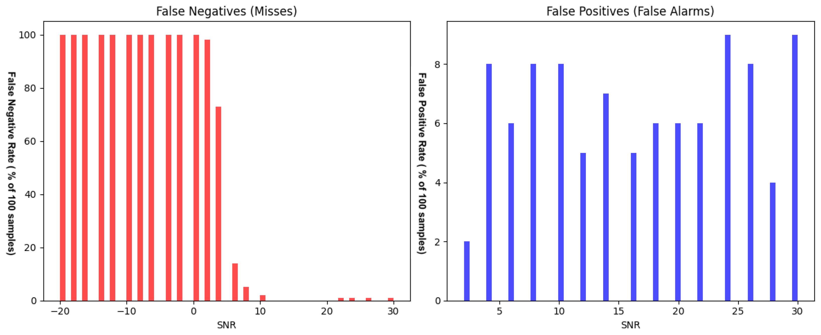
Experiment 3 trains a detector directly on multi-signal data. Any sample containing a BPSK component (pure BPSK or BPSK+QPSK mixture) is labeled positive, while all other signals are labeled negative. This experiment evaluates whether explicit exposure to interference can restore detection capability. The false positive and false negative rates are shown in Figure 3.

The multi-signal detector recovers detection on mixtures (Table 3, class 24 under “Multi-Signal(2)”) while maintaining comparable performance on pure BPSK. However, Table 2 also shows that multi-signal training can induce false positives on certain AM sideband classes (classes 17 and 18). This is a significant observation, as it suggests that the underlying issue may not originate from the BPSK or QPSK modulation schemes themselves, but rather from another part of the system (a different modulation that the superposition resembles).

To mitigate these confusions, an extended discriminator set is introduced by including closely related modulation types in training (Table 3, classes 25 and 26 under “Multi-Signal”). This modification increases the number of true positives for the target signal from 50.04% in the two-signal case to 53.15%. It also reduces false positives for classes 17 and 18 from 8.88% and 9.08% to 0.04% and 0.81%, respectively.

This behavior further supports the underlying premise of this work: the detector’s performance is strongly influenced by the diversity and structure of the training data. Rather than being a limitation of the BPSK–QPSK pairing itself, the observed confusions highlight that the model learns decision boundaries based on the set of modulations it is exposed to. By expanding the discriminator set, the model is able to better allocate capacity and refine these boundaries, improving both true positive rates and false alarm control. This reinforces the idea that targeted data design, rather than simply increasing model complexity, is critical for robust detection in realistic multi-signal environments.

As shown in the formulations, the attention mechanism can separate different signal components based on their learned structure. The experimental results confirm that the model is able to distinguish between classes under multi-signal conditions.

6.4. Summary of Evaluated Scenarios

Table 2 summarizes confusion matrix values for all evaluated scenarios, including baseband versus mixed-frequency conditions, sampling-rate mismatches, early-exit inference, multi-signal training, and transfer learning.

6.5. Early-Exit Inference

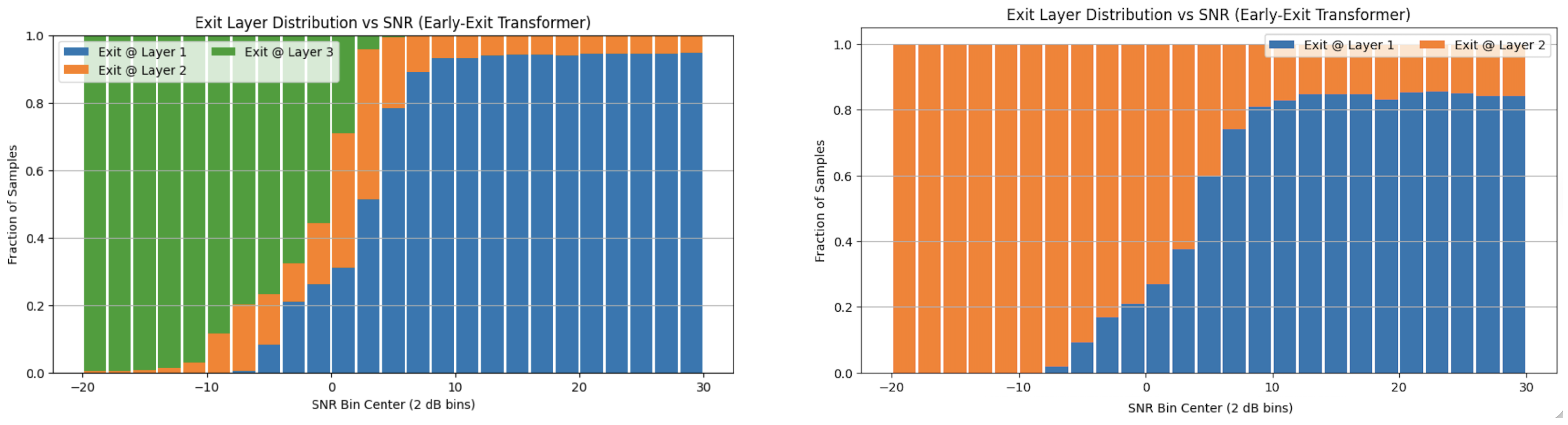
Transformer inference is expensive because all encoder layers must be executed for every input. Many samples are easy to classify (especially at high SNR), motivating an early-exit strategy [32]: intermediate classifiers are attached to early layers and inference stops once confidence exceeds a threshold. Figure 4 illustrates early-exit behavior across SNR values.

At high SNR, approximately 80% of samples exit early, substantially reducing average computation. Table 2 shows that early-exit inference preserves detection performance and, in some cases, slightly improves TN/TP (e.g., “Baseband Train/Test, Early Exit” and “Mixed Train/Test, Early Exit”).

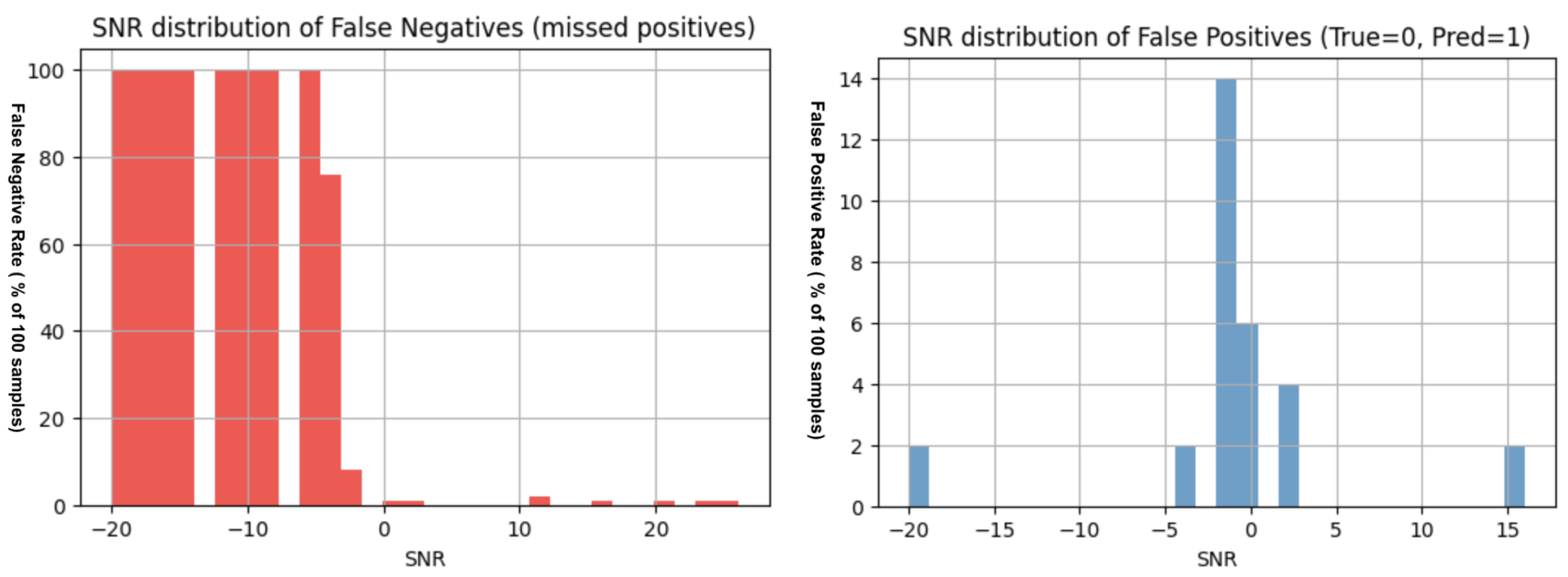
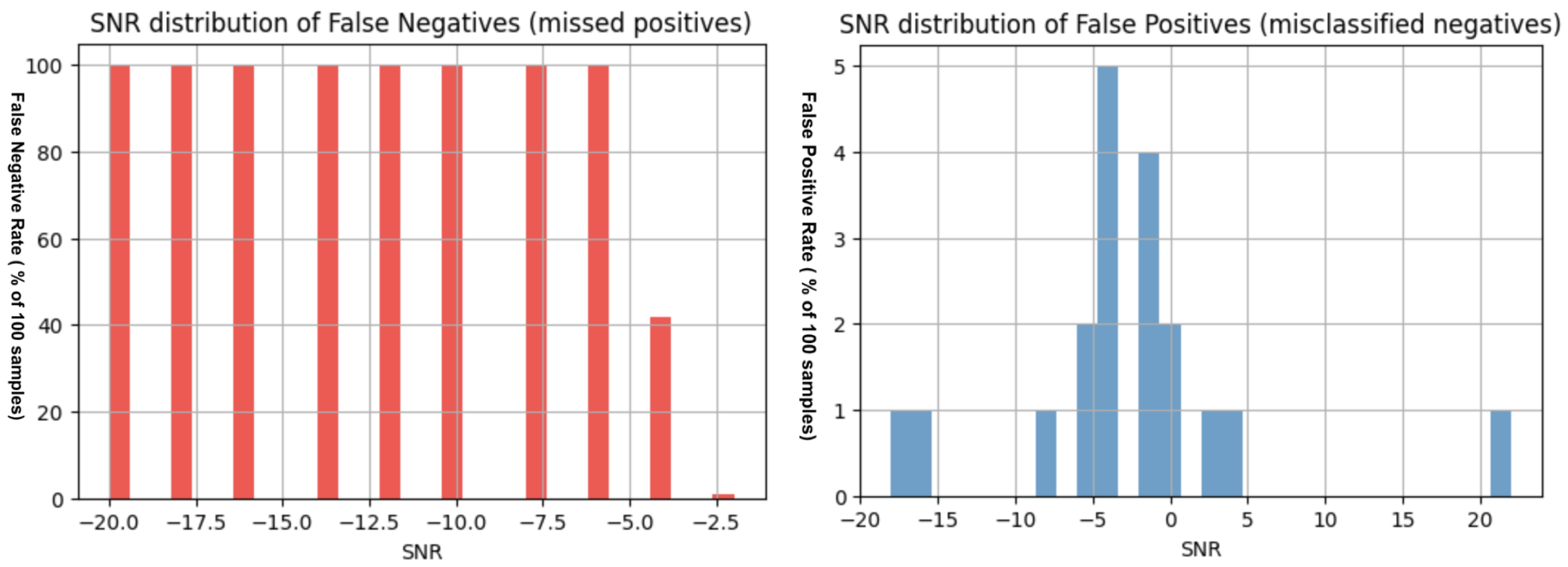
As with the standard transformer, most early-exit errors are concentrated at low SNR values. Figure 5 and Figure 6 illustrate the false negative and false positive behavior across SNR values for the mixed-frequency and baseband scenarios, respectively.

To clarify the nature of this efficiency gain, the benefit of early-exit inference should not be interpreted as a fixed speedup, but rather as adaptive computation conditioned on signal difficulty. In the evaluated setting, a large fraction of high-SNR samples exit at early layers, indicating that the model can confidently classify these inputs without utilizing the full network depth. In contrast, lower-SNR or more complex samples continue through the entire model.

This behavior induces a dynamic allocation of computational resources: easy signals (high SNR) require fewer operations, while hard signals (low SNR) retain full computational processing. As a result, the average computational cost is reduced, even though the worst-case cost remains unchanged.

Importantly, this represents a gain in resource efficiency rather than a strict reduction in worst-case latency. The model avoids unnecessary computation on easy samples, enabling available resources to be redirected toward more challenging inputs or parallel processing tasks. This property is advantageous in real-world RF systems, where computational budgets are constrained, and signal conditions vary significantly over time.

6.6. Comparison with a 24-Class Transformer Model

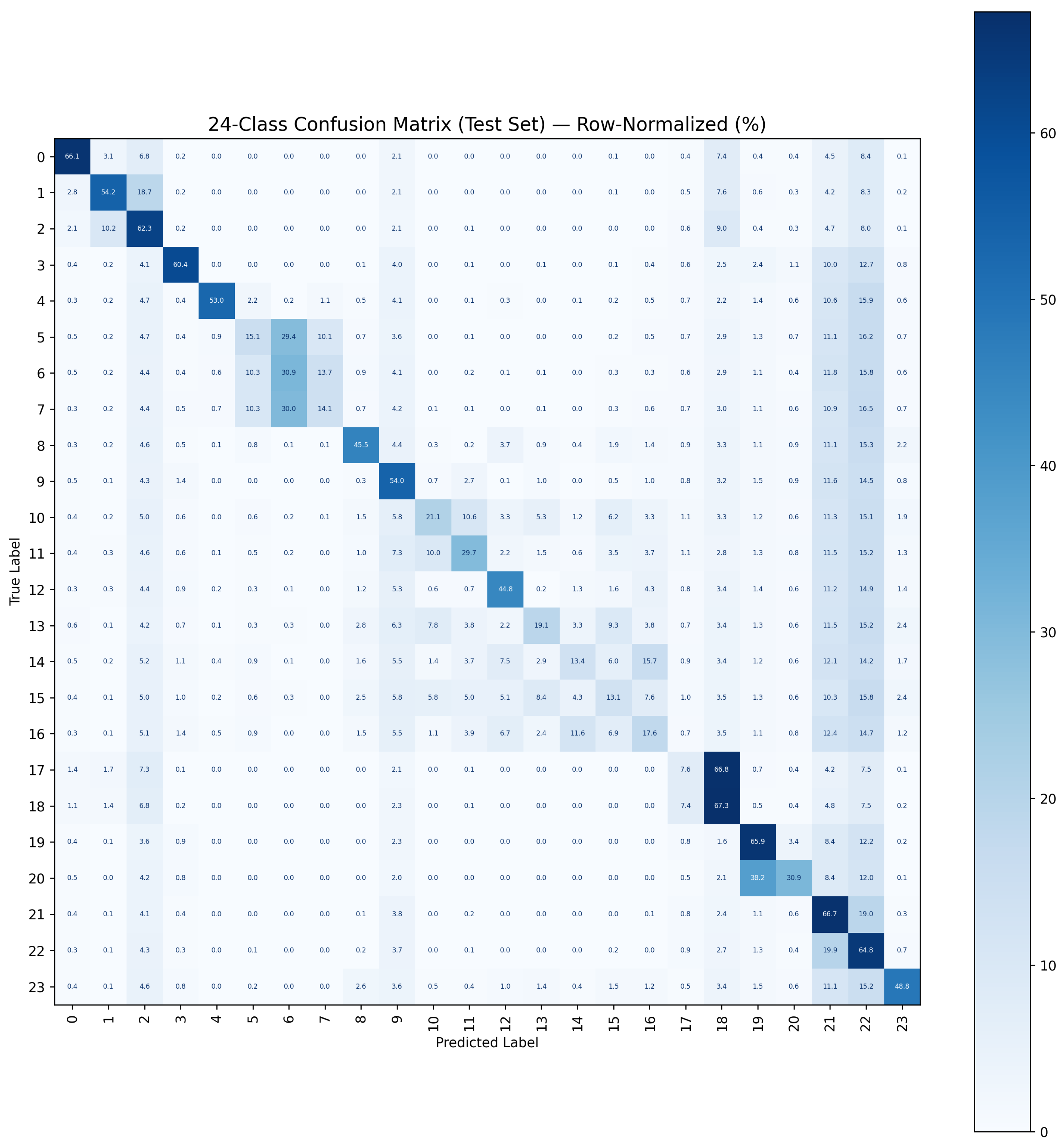
For reference, a conventional 24-class transformer model is trained to predict one of the 24 modulation classes. The same approach as earlier was used, except that the problem was formulated as a 24-class output layer instead of the earlier binary class classifier. The confusion matrix of a 24-class classifier is shown in Figure 7.

In this study, the binary detectors generally provide stronger SOI-versus-background discrimination than the 24-class model. A likely contributing factor is that the same hyperparameter scale is used, whereas multi-class classification typically requires higher-capacity models to learn separations across many classes.

Class 3 achieved a false positive rate of 14% and a false negative rate of 38%. For the binary classifier, the detection rate has a false positive rate of 0.09% and a false negative rate of 1.42%. Binary detectors are generally better suited for identifying features associated with a single class, rather than distinguishing across multiple classes, particularly when operating under the same architectural constraints. This result reflects a capacity-allocation effect: if model size is fixed, binary detectors can devote capacity exclusively to the SOI-specific discrimination, whereas multi-class models must distribute capacity across all the 24 decision boundaries.

While the approach can be generalized to other model architectures, the intent of this study is not to perform an exhaustive comparison across models, but to clearly demonstrate the underlying principle under controlled conditions.

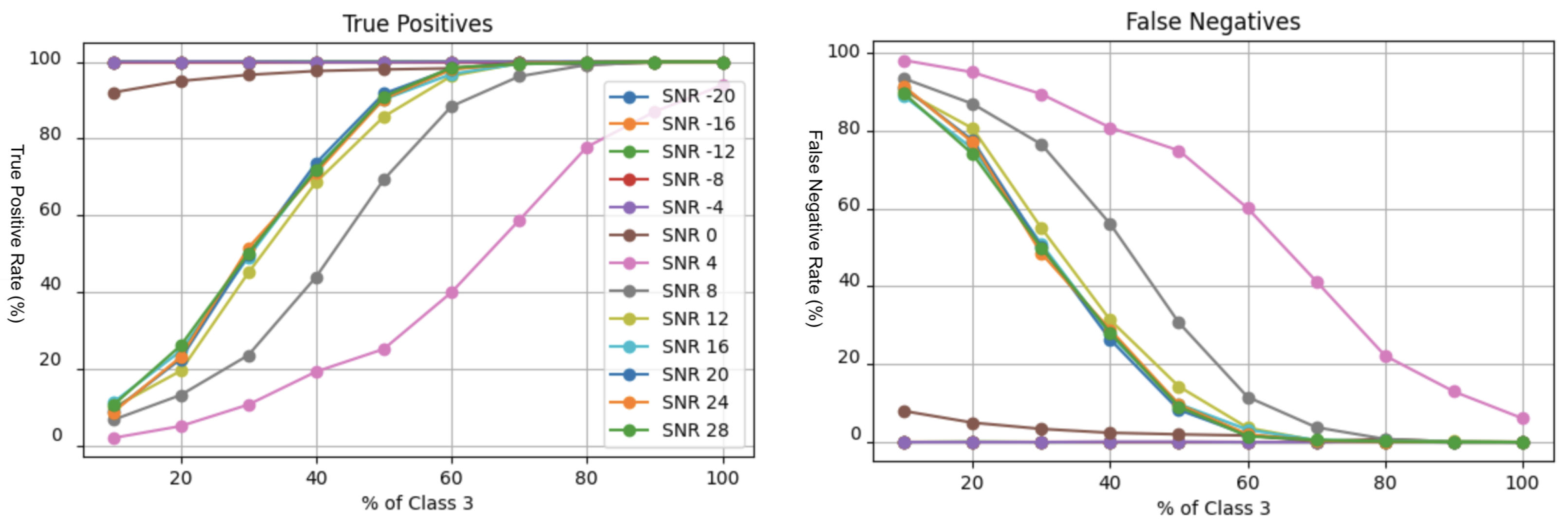
6.7. Time-Domain Contamination Study

The previous multi-signal experiments considered simultaneous transmissions (overlap in time) at different center frequencies. This study instead examines temporal co-occurrence at baseband: the SOI (BPSK) occupies the beginning of the window and a second modulation (QPSK) occupies the remainder. By varying the fraction of the window containing BPSK, we evaluate how much uncontaminated SOI content is required for reliable detection. The true positive and false negative behavior as a function of contamination is illustrated in Figure 8.

As expected, robustness improves as the proportion of SOI content increases. Importantly, temporal co-occurrence has a smaller impact than spectral co-occurrence: when modulations are separated in time, the SOI segment remains uncontaminated and its phase/amplitude structure is more readily detected.

6.8. Transfer Learning

Transfer learning is investigated as a means of efficiently training detectors for additional modulations. Given the structural similarity between BPSK and QPSK, a detector pretrained on BPSK might be expected to adapt to QPSK with limited retraining. If successful, this approach would reduce the need to train every modulation from scratch, enabling scalable deployment by training only a subset of representative signals and adapting them to others.

Two transfer learning strategies are evaluated: (i) partial fine-tuning of the backbone network by retraining a limited subset of layers (specifically, the final two layers) while keeping the remaining layers fixed, and (ii) retraining only the early-exit classifiers while preserving the backbone network parameters.

For the first strategy, the results indicate a substantially elevated false positive count of 81.68%, which is the highest observed across all evaluated experiments. A plausible explanation is that the model has been strongly optimized for BPSK detection; introducing QPSK as a new target while keeping early feature representations fixed may bias the network toward patterns previously associated with positive detections. Consequently, the decision boundary shifts in a manner that significantly increases false alarms across all classes. This reflects a common issue in signal classification: when two modulation schemes are superimposed, they can introduce composite features that resemble those of a third or fourth modulation type. As a result, the root cause of the misclassification may stem from signal superposition effects rather than from deficiencies in the individual modulation schemes themselves.

Partial retraining of the backbone by fine-tuning the final two layers yields a notable reduction in false positives to 23.98%. While this represents an improvement, the false positive rate remains unacceptably high relative to other evaluated configurations.

This outcome is problematic for signal detection applications, where false alarms are highly undesirable. Each false positive typically requires additional verification, increasing operational burden and reducing system efficiency. As such, the current transfer learning approaches examined here require further refinement before they can be considered viable for accelerated training of related modulations. Overall, these results highlight a key limitation: transfer learning does not generalize effectively across distinct modulation classes in this setting.

Transfer learning may still be effective when applied within the same modulation family or task domain. To evaluate this hypothesis, the baseband BPSK detector was employed as a pretrained model and subsequently adapted to more complex signal environments. Specifically, it was fine-tuned on mixed-signal data derived from baseband conditions, as presented in Table 2 (Transfer Learning, Early Exit (Baseband→Mixed BPSK)). The early-exit retraining approach yielded 3.51% true positives but an excessive 57.72% false positives, indicating no meaningful improvement. In contrast, retraining the final two layers reduced false positives to 0.8%, while achieving 1.88% true positives and 2.33% false negatives, representing a substantial improvement in false-alarm control, as presented in Table 2 (Transfer Learning, Last Two Layers (Baseband→Mixed BPSK)).

In this experiment, the Mixed Signal Model was trained and evaluated exclusively on baseband-shifted data, without exposure to multi-signal interference, and then applied directly to a multi-signal detection scenario. Despite this training–deployment mismatch, the model achieved a 67.37% sensitivity and 49.86% precision, indicating reasonably strong baseline performance given that the model had never been exposed to multi-signal data during training. In Experiment 2, a transfer-learning strategy was employed in which the final two layers of the same model were retrained, enabling targeted adaptation to the multi-signal environment. This approach yielded 75.27% sensitivity and 87.7% precision, demonstrating a substantial improvement in detection capability and a pronounced reduction in false alarms achieved through limited fine-tuning rather than architectural modification. The results are presented in Table 2 under the scenario “Transfer Learning, Early Exit (Mixed BPSK→Multi-Signal)” and “Transfer Learning, Last Two Layers (Mixed BPSK→Multi-Signal).”

Table 4. Original class distribution versus binary prediction percentages. Red entries correspond to highlighted values in the plots. All values are reported as percentages relative to the original class size.

Class	Early Exit (BB→Mixed)		2-Layer (BB→Mixed)		Early Exit (Mixed→Multi)		2-Layer (Mixed→Multi)
	P0 (%)	P1 (%)	P0 (%)	P1 (%)	P0 (%)	P1 (%)	P0 (%)	P1 (%)
0 (OOK)	39.38	60.62	100.00	0.00	45.42	54.58	99.73	0.27
1 (4ASK)	58.35	41.65	100.00	0.00	64.23	35.77	98.04	1.96
2 (8ASK)	58.81	41.19	100.00	0.00	74.31	25.69	98.85	1.15
3 (BPSK)	15.69	84.31	55.38	44.62	48.31	51.69	45.77	54.23
4 (QPSK)	51.77	48.23	99.00	1.00	99.88	0.12	99.81	0.19
5 (8PSK)	51.88	48.12	100.00	0.00	99.92	0.08	99.85	0.15
6 (16PSK)	51.42	48.58	100.00	0.00	99.96	0.04	99.85	0.15
7 (32PSK)	52.31	47.69	99.96	0.04	99.88	0.12	99.88	0.12
8 (16APSK)	34.62	65.38	99.73	0.27	99.65	0.35	99.54	0.46
9 (32APSK)	8.31	91.69	97.65	2.35	98.15	1.85	95.23	4.77
10 (64APSK)	12.35	87.65	99.27	0.73	99.42	0.58	99.54	0.46
11 (128APSK)	8.92	91.08	99.42	0.58	99.69	0.31	99.46	0.54
12 (16QAM)	13.73	86.27	99.31	0.69	99.42	0.58	99.15	0.85
13 (32QAM)	14.31	85.69	98.92	1.08	99.65	0.35	99.19	0.81
14 (64QAM)	9.58	90.42	99.19	0.81	99.54	0.46	98.19	1.81
15 (128QAM)	11.50	88.50	99.15	0.85	99.38	0.62	99.15	0.85
16 (256QAM)	9.27	90.73	99.23	0.77	99.46	0.54	98.96	1.04
17 (AM-SSB-WC)	61.08	38.92	100.00	0.00	94.42	5.58	98.00	2.00
18 (AM-SSB-SC)	61.15	38.85	100.00	0.00	94.08	5.92	98.65	1.35
19 (AM-DSB-WC)	19.00	81.00	99.19	0.81	99.27	0.73	99.92	0.08
20 (AM-DSB-SC)	16.19	83.81	98.19	1.81	99.38	0.62	99.85	0.15
21 (FM)	55.54	44.46	100.00	0.00	99.96	0.04	99.88	0.12
22 (GMSK)	55.23	44.77	100.00	0.00	99.96	0.04	99.88	0.12
23 (OQPSK)	38.85	61.15	97.35	2.65	99.42	0.58	98.27	1.73
24 (BPSK+QPSK)	–	–	–	–	16.96	83.04	3.65	96.35

summarizes the class-wise binary prediction percentages for the evaluated transfer learning configurations.

7. Discussion

7.1. Key Empirical Findings

The experiments demonstrate that realistic RF conditions substantially alter detector behavior compared to the idealized baseband, single-signal setting typically assumed in public benchmarks. Three findings are important for practitioners.

First, center-frequency shifts are a major failure mode when they are not represented during training. A detector trained only on baseband recordings does not generalize to frequency-shifted signals: missed detections increase sharply and true positives collapse. This indicates that a “train at baseband, deploy anywhere” assumption is not valid for the evaluated transformer configuration, and that either explicit data augmentation (frequency mixing) or an operational downconversion stage is required.

Second, sampling-rate mismatch consistently degrades performance, with larger penalties as the resampling ratio deviates further from one. While moderate mismatch may be tolerable, the results suggest that resampling artifacts (especially interpolation in the mixed-frequency setting) can be disruptive. This emphasizes that practical RFML deployments should treat sampling-rate assumptions as part of the model specification: the front-end resampling strategy and the classifier should be designed and validated together.

Third, simultaneous multi-signal mixtures can cause complete detection failure unless the interference structure is explicitly modeled during training. When a second modulation co-occurs at a different center frequency, a detector trained only on single-signal examples can fail to identify the SOI altogether. Training directly on multi-signal mixtures restores detection capability, but it can introduce new confusions (e.g., elevated false positives for certain AM sideband classes). Extending the discriminator set with “hard negative” mixture classes reduces these false alarms, illustrating that discriminator selection is central to robust binary detection.

Two additional observations refine the above points. The time-domain contamination study shows that co-occurrence in time is less damaging than co-occurrence in frequency: when the SOI occupies a sufficient fraction of the window, detection remains reliable because a contiguous, uncontaminated segment retains the phase/amplitude structure required for recognition. Early-exit inference provides a meaningful efficiency gain: high-SNR samples often reach high confidence at early layers (Figure 4), reducing average computation while preserving (and in some cases slightly improving) overall detection metrics.

Finally, transfer learning does not generalize effectively across inter-modulation tasks, suggesting that distinct modulation types may require independent training. In contrast, transfer learning performs well for intra-modulation scenarios, such as adapting a baseband model to operate in a mixed-signal environment or extending a mixed-signal model to a multi-signal setting.

7.2. Scope of Baseline Comparisons

The baseline comparisons in this study are intentionally designed to isolate the impact of task formulation rather than to benchmark architectural performance. Specifically, the comparison with a 24-class transformer model is conducted under a similar hyperparameter budget to control for model capacity, enabling a focused evaluation of the binary versus multi-class formulation.

We acknowledge that additional baselines, such as CNN- or LSTM-based models, as well as lightweight classifiers (e.g., support vector machines with hand-crafted features), could further enrich the study. However, the primary objective of this work is to evaluate a task-aligned binary signal-of-interest (SOI) detection framework under realistic RF impairments, rather than to establish state-of-the-art performance across architectures. The goal is to replace handcrafted classifiers with transformer-based models that can leverage GPU acceleration for real-time and scalable signal detection.

In contrast to much of the existing AMC literature, which primarily evaluates models under idealized single-signal, baseband conditions (e.g., RadioML datasets), this work emphasizes more realistic scenarios, including mixed-frequency, sampling-mismatched, and multi-signal environments. Under these conditions, model behavior is strongly influenced by task formulation, and the results demonstrate that a binary SOI detection approach improves robustness and interpretability.

The use of a relatively simple, general-purpose architecture is also deliberate. This avoids reliance on hand-crafted feature pipelines or highly specialized models that may not generalize well across environments, and instead supports an end-to-end learning framework operating directly on raw IQ data.

From a systems perspective, the proposed approach offers several practical advantages. It enables modular deployment, where detectors can be trained and updated independently for different signals of interest; adaptability, where models can be retrained or fine-tuned for new RF conditions such as mixed or multi-signal environments; and scalability, where only relevant detectors need to be deployed for a given band or operational scenario.

Finally, transformer-based models provide an additional implementation advantage: they are highly amenable to parallel computation on modern GPU hardware. Unlike sequential models such as LSTMs, transformers process entire input sequences simultaneously, enabling efficient training and inference at scale. This property is particularly beneficial for real-time or large-scale RF monitoring systems, where throughput and parallel processing capability are critical.

The conclusions of this study are primarily derived from experiments using BPSK as the signal of interest, and therefore may not directly generalize to all modulation types. Different modulation schemes exhibit distinct statistical and structural properties, and their behavior under realistic RF impairments can vary significantly. In particular, modulation families such as AM and FM introduce additional complexity due to continuous amplitude or frequency variations, which may not be captured by models optimized for discrete phase-modulated signals.

Furthermore, in multi-signal environments, the superposition of signals can produce composite patterns that are difficult—or in some cases practically impossible—to separate, depending on factors such as relative power levels, frequency offsets, and temporal overlap. Additional signal characteristics, including baud rate and symbol timing, are also not explicitly modeled in this study and may influence detection performance.

The scope of this work is intentionally narrowed to enable controlled analysis under multiple interacting RF impairments across a large set of modulation classes. Given the diversity and complexity of the 24 modulation types in the dataset, this focused approach allows for clearer interpretation of task formulation effects.

These limitations also point to future research directions. More complex and heterogeneous scenarios—such as overlapping radar and communication signals (e.g., FMCW radar coexisting with LTE transmissions)—represent important real-world conditions that warrant further investigation. Additionally, the results suggest that modulation-aware or hybrid architectures, incorporating signal-processing-informed inductive biases and tailored to specific signal families, represent a promising direction for improving performance beyond fully general-purpose models.

7.3. Scalability and Deployment Considerations

A potential concern with the proposed modular approach is that a bank of K independent binary detectors may incur higher total computational cost than a single K-class model. In the worst case, evaluating all detectors sequentially would scale linearly with K.

However, the proposed framework is not intended for uniform, always-on deployment of all detectors. In realistic spectrum monitoring systems, detectors can be selectively deployed based on prior knowledge of the frequency band, operational context, or upstream signal detection stages. Because each detector focuses on a single SOI against a background set, model capacity and training effort can be concentrated where it matters operationally. As a result, only a subset of detectors is active, making the effective computational cost substantially lower than the worst-case bound. Furthermore, the architecture naturally supports parallel execution across hardware resources, allowing efficient scaling in high-throughput settings.

Additionally, the binary formulation enables:

• Parallelization: detectors can be distributed across hardware resources or evaluated concurrently,
• Incremental deployment: new signals of interest (SOIs) can be added without retraining a global model,
• Reduced model complexity per task: each detector learns a simpler decision boundary (SOI vs. background).

We acknowledge these considerations and emphasize that the proposed framework is designed for practical deployment scenarios, where simplicity, adaptability, and selective activation are prioritized over uniform full-scale operation. A key advantage of the binary formulation is that detectors can be trained under simple conditions (e.g., baseband) and incrementally adapted to more complex environments (e.g., mixed-frequency or multi-signal) without retraining a monolithic multi-class model. From a systems perspective, this replaces a single rigid model with a collection of smaller, specialized detectors that can be composed as needed, allowing model complexity to scale with environmental demands.

Resolution of decision conflicts: In scenarios where multiple detectors produce positive outputs for the same input, this is not necessarily an error condition but may reflect true multi-signal coexistence. Nevertheless, several resolution strategies are available:

• Confidence-based selection: selecting the detector with the highest posterior probability,
• Threshold calibration: tuning detector-specific thresholds to control false positives,
• Multi-label interpretation: allowing multiple simultaneous positives in multi-signal environments,
• Hierarchical or downstream verification: applying secondary classifiers or signal separation methods.

The appropriate strategy depends on the application (single-emitter vs. multi-emitter environments), and the modular framework allows this policy to be adapted without retraining models.

The results also show that binary detection is not “set and forget.” The discriminator set must reflect the RF environment the detector will see. In multi-signal scenarios, including realistic hard negatives (e.g., likely co-occurring modulations and mixture classes) can substantially reduce false alarms. This mirrors classical detection practice, where the most important confusers are explicitly modeled. From an engineering standpoint, it suggests that deploying detector banks should be accompanied by a process for updating discriminators as spectrum occupancy evolves.

7.4. Why Inter-Modulation Transfer Learning Fails

Inter-modulation transfer learning fails primarily due to modulation-specific feature learning and decision boundary mismatch. Although BPSK and QPSK are closely related modulation schemes, this represents a challenging transfer scenario. BPSK consists of two constellation phase points, whereas QPSK introduces four phase states, resulting in a fundamentally richer phase structure. While this difference appears small in the signal domain, it induces a significant shift in the learned representation space.

From the perspective of the self-attention mechanism (Section 4), the model effectively learns a data-driven approximation to complex correlation, where attention weights depend on phase relationships of the form $\cos \left(\varphi \right[n]-\varphi [m\left]\right)$. For BPSK, phase transitions are constrained to two discrete states, producing a relatively simple and highly structured phase-difference distribution. In contrast, QPSK introduces additional phase transitions (e.g., $\pm \pi /2$ shifts), leading to a more complex and less predictable phase relationship across time.

Several factors contribute to the observed transfer failure. First, feature specialization causes the model to learn phase transition patterns that are tightly coupled to the BPSK phase structure. Because attention weights implicitly encode phase coherence, the learned similarity function becomes tuned to BPSK-specific phase differences and does not generalize to the broader phase set of QPSK.

Second, decision boundary bias arises because the pretrained model is optimized for a “BPSK versus background” task. This results in a representation space in which BPSK-like phase coherence patterns are strongly emphasized. When retargeted to QPSK, samples that partially resemble BPSK phase behavior can be incorrectly classified as positive, leading to elevated false positive rates, as observed in Table 2.

Third, limited adaptability during partial fine-tuning further restricts performance. When only the final layers are retrained, earlier layers—responsible for encoding phase relationships through attention—remain fixed. As a result, the model cannot adjust its underlying phase-similarity function to accommodate the different constellation geometry of QPSK.

Finally, in multi-signal environments, composite feature effects further degrade transfer performance. As shown in Section 3.8, the superposition of multiple signals introduces cross-terms with oscillatory phase components. These interactions can generate emergent phase/amplitude patterns that do not correspond to any single modulation class, increasing the likelihood of misclassification.

Overall, these results indicate that inter-modulation transfer is fundamentally difficult, even between closely related schemes such as BPSK and QPSK, because the learned attention-based representations are highly modulation-specific and tightly coupled to phase structure.

7.5. Implications for End-to-End Spectrum Monitoring

These findings support a systems-oriented view in which modulation detection/classification is preceded by signal detection and isolation. In wideband spectrum monitoring, candidate signal emissions are commonly localized in the time–frequency domain using classical energy detection techniques [35] or spectrogram-based methods. Recent work has extended object-detection frameworks from computer vision to RF spectrograms, where emissions are treated as visual objects and localized using bounding-box detectors such as Faster R-CNN, YOLO, and transformer-based architectures [36,37,38]. In parallel, traditional image-processing and unsupervised approaches, including thresholding and clustering methods such as k-means, remain widely used for grouping energy concentrations into candidate signal regions. Once a contiguous region is isolated, a modulation detector can be applied on a narrower bandwidth segment where the number of co-occurring signals is reduced. Vision Transformer approaches have also been applied to RF spectrograms by treating signals as images [39].

After isolation, two practical processing paths exist. The first is to mix the isolated band to baseband and then apply a baseband-trained detector. This approach leverages the simplicity of baseband representations but depends on accurate downconversion and adequate filtering. The second path is to classify the filtered signal directly at its observed center frequency using a detector trained with frequency offsets. This avoids additional mixing and can be advantageous when downconversion is imperfect or when center-frequency alignment varies across captures.

Filtering and band isolation play an important role in both paths. In practice, filter cutoffs may not be perfectly centered around the desired emission, and nearby signals or leakage can remain in-band. FIR filters can provide linear phase (often desirable for preserving waveform structure) but may require more taps and higher computational cost; IIR filters can be more efficient but introduce nonlinear phase distortion. The experiments in this paper highlight that even modest residual interference can change detector behavior, motivating an integrated design philosophy: filtering, downconversion (if used), and detector training should be co-designed so that the detector is exposed to the residual artifacts expected at deployment.

7.6. Architectural Design Considerations

Architectural design choices and opportunities for innovation: The present study intentionally adopts a standard Transformer backbone to isolate the impact of the problem formulation (binary detection under realistic RF impairments) from architectural modifications. This allows the observed performance gains to be attributed directly to data modeling and training strategy rather than to architecture-specific optimizations.

However, the analysis in Section 3 suggests that self-attention over IQ samples implicitly approximates complex correlation and phase-difference computations. This observation opens several directions for domain-specific architectural improvements:

• Physics-informed attention: incorporating explicit complex-valued or phase-aware operations (e.g., learned approximations of $x\left[n\right]x^{*}\left[m\right]$) to better capture modulation structure,
• Channelizer-inspired front-ends: integrating learned or hybrid polyphase filterbanks to provide frequency-localized representations prior to attention,
• Frequency-offset estimation modules: introducing components that explicitly model and compensate for carrier frequency offset (CFO) or drift,
• Lightweight attention mechanisms: reducing computational cost via sparse attention, reduced head counts, or structured attention tailored to temporal locality,
• Binary-specific heads: designing output layers optimized for SOI-versus-background discrimination rather than multi-class separation.

More concretely, future architectures could combine signal processing structure with learning by embedding operations such as:

$$x\left[n\right]·e^{-j\widehat{\omega }n},\widehat{\omega }\approx \mathrm{learned}\mathrm{frequency}\mathrm{offset},$$

(44)

or by explicitly modeling phase differences:

$$\Delta \varphi (n,m)=\arg \left(x\left[n\right]x^{*}\left[m\right]\right),$$

(45)

within the network. Such designs would move beyond generic Transformers toward hybrid model-based + data-driven RF architectures.

7.7. Limitations and Future Work

Several limitations frame the scope of these conclusions. First, the study uses synthetically generated frequency shifts and mixtures derived from the RadioML dataset. While this enables controlled experiments, it does not capture the full diversity of over-the-air impairments such as hardware nonlinearities, phase noise, carrier frequency drift dynamics, nonstationary noise, and multipath fading. Second, the experiments anchor on a single SOI (BPSK) to enable a focused analysis; extending the study across additional modulations would further clarify which trends are universal versus modulation-specific. Third, the early-exit mechanism provides limited benefit in low-SNR regimes where confidence is inherently low; complementary approaches such as uncertainty estimation, calibration, or joint detection/denoising may be needed when low-SNR performance is critical.

Future work can therefore proceed in three directions: (i) evaluation on over-the-air captures and hardware-in-the-loop datasets; (ii) richer augmentation strategies that jointly model frequency offset, sampling-rate offset, fading, and interference statistics; and (iii) scalable procedures for building detector banks, including principled discriminator selection, continual learning for evolving bands, and lightweight calibration to control false alarms under distribution shift.

Positioning of this work: This paper establishes a strong baseline by demonstrating that a standard Transformer, when paired with an appropriate binary detection formulation and realistic data modeling, already exhibits robustness to frequency shifts and multi-signal interference. The proposed framework therefore, serves as a foundation upon which more specialized, RF-aware architectures can be developed.

8. Conclusions

This work reframes automatic modulation classification as a targeted binary detection problem and evaluates transformer-based detectors under progressively realistic RF conditions. The results highlight a consistent gap between benchmark-style assumptions and practical deployment scenarios. In particular, models trained on idealized baseband data fail to generalize to center-frequency offsets and multi-signal interference, demonstrating that explicit modeling of these effects is not optional but necessary for reliable operation. Across experiments, center-frequency shifts and spectral co-occurrence emerge as the most disruptive factors, often leading to near-complete detection failure when not represented in training. In contrast, time-domain co-occurrence is less detrimental, provided that a sufficient portion of the signal of interest remains uncontaminated. These findings reinforce that the structure and diversity of training data—not just model architecture—play a dominant role in determining real-world robustness. The proposed binary detection framework offers a practical alternative to conventional multi-class classifiers by focusing model capacity on signals of interest and reducing unnecessary inter-class confusion. This is particularly important in operational settings where only a subset of modulations is relevant. Early-exit inference further improves the feasibility of deployment by enabling adaptive computation, reducing average inference cost in high-SNR regimes without sacrificing performance. Transfer learning results indicate that while intra-modulation adaptation (e.g., baseband to mixed conditions) is feasible, generalization across different modulation types remains limited and can introduce significant false alarms. This suggests that scalable deployment will likely require either carefully structured training curricula or modulation-aware adaptation strategies rather than naive reuse of pretrained detectors. Overall, the results support a system-level design in which traditional RF front-end processing (e.g., detection and isolation) is combined with modular, SOI-specific binary detectors trained on realistic signal conditions. Future work should extend this framework to a broader set of modulations, incorporate more diverse interference scenarios, and explore architectures that explicitly account for frequency variability and multi-signal structure.