Wavelet Basis Selection in Signal Denoising Based on Wavelet-Coefficient Distribution Shape

Abstract

Denoising one-dimensional signals by wavelet shrinkage critically depends on the choice of wavelet basis, yet basis selection is often guided by heuristics rather than explicit statistical criteria. This paper investigates the relationship between wavelet-basis properties and the shape of the probability density function (PDF) of the detail coefficients in the coarsest retained detail subband. On this basis, it proposes the shape of this PDF as a criterion for wavelet-basis selection. We hypothesize that, for a fixed decomposition depth, noise model, and shrinkage rule, a basis better matched to the signal’s local regularity produces a narrower and more sharply peaked coefficient PDF in this subband than a mismatched basis and can therefore serve as a data-driven indicator for basis selection. To evaluate the consistency of this proposal, we perform controlled hard-thresholding experiments on six canonical test signals, five wavelet bases, and additive white Gaussian noise. Although the test signals differ significantly in local regularity and features, the relationship between basis suitability and PDF shape is confirmed for each of them. Therefore, the results suggest that the proposed PDF-shape criterion is a valuable indicator for wavelet-basis selection.

1. Introduction

Denoising of one-dimensional (1-D) signals is a common problem in signal processing. Wavelet-domain shrinkage and Bayesian estimation are widely used because they adapt to local regularity while preserving discontinuities. They are applied both as standalone methods and as components in ensemble schemes or hybrid approaches that incorporate deep learning [1]. Wavelet bases provide multiscale, localized representations in which smooth components concentrate into a few large coefficients, whereas noise and fine-scale irregularities appear as many small coefficients. Choosing an appropriate wavelet basis is therefore critical for achieving high-quality results, especially for denoising algorithms that are expected to handle multiple signal classes with differing characteristics.

A well-established design principle is that longer, smoother wavelet functions (with more vanishing moments) are preferable for smoother signals with few or no edges, whereas shorter, less smooth wavelets work better for signals with sharp transitions. If a long, smooth basis is used for a signal with edges, edge smearing and ringing artifacts can occur. On the other hand, if short bases with compact support are used for smooth signals, staircase artifacts and weaker noise suppression can occur. This behavior follows from the trade-off between regularity and compact support imposed by filter-bank constructions and vanishing-moment constraints [2,3,4,5].

The importance of the basis selection has also been explored in recent studies. Sahoo et al. formalize optimal wavelet choice for signal denoising via multi-criteria selection (energy compaction, correlation, and edge retention), showing that basis choice alone can yield substantial RMSE improvements before threshold tuning [6], while Abdelfattah et al. propose seamless optimization of wavelet parameters for LFM radar signals, automatically selecting filter length and shape to balance sidelobe suppression and noise removal [7].

It is shown in [5,8,9,10] that wavelet coefficients of both real and synthetic data typically exhibit distinctly non-Gaussian, heavy-tailed behavior. Commonly, generalized Gaussian distributions (GGDs) and Gaussian scale mixtures are used to provide accurate parametric descriptions of marginal statistics. Although these models were developed primarily for images, their conclusions transfer to 1-D signals: at fine scales dominated by noise, empirical coefficient PDFs are nearly Gaussian, whereas at coarser scales containing structured signal content, the PDFs sharpen and become increasingly leptokurtic. Consequently, the shape of the coefficient PDF conveys information about both the signal–noise composition and the suitability of the chosen basis for representing the underlying signal structure [4,11].

In this paper, we introduce the hypothesis that the shape of the PDF of the detail coefficients in the coarsest retained detail subband (hereafter referred to as the last decomposition level) carries sufficient information to be used as a tool for selecting wavelet bases in 1-D signal denoising. Concretely, for a fixed noise level and thresholding strategy, we posit that a basis well matched to the signal’s local regularity yields a coefficient PDF at the last level that is narrower and more peaked than that of a mismatched basis. The hypothesis is consistent with three complementary lines of prior work. First, classical shrinkage theory links basis adaptivity to risk: orthonormal wavelet bases endowed with appropriate regularity enable near-minimax denoising for smooth signals [2,11]. Second, empirical and Bayesian thresholding methods model the shape of coefficient PDFs explicitly (e.g., GGD, Laplacian, or GSM) and derive data-adaptive thresholds that exploit subband-wise or interscale statistics [5,9,10]. Third, redundancy and translation invariance (cycle spinning and stationary transforms) stabilize coefficient statistics and reduce artifacts near singularities, further clarifying PDF shape at coarse scales [3,4].

Section 2 presents basics of wavelet basis selection and introduces a suite of test signals, Section 3 details the analysis of the PDF shape and influencing factors, and Section 4 discusses experimental results and the hypothesis validity.

2. Wavelet Regularity, Support, and Suitability to Signal Classes

It is well established that the structural properties of an orthonormal wavelet basis—particularly the number of vanishing moments, pointwise regularity, and compact support length—govern its suitability for denoising signals of differing smoothness and edge content [2,12,13,14]. Let $\psi$ denote a mother wavelet with m vanishing moments,

$${\int }_{\mathbb{R}}{t}^k\psi \left(t\right)dt=0,k=0,1,\dots ,m-1,$$

(1)

and let ${\psi }_{j,k}\left(t\right)=2^{-j/2}\psi (2^{-j}t-k)$ be its dilates and translates. Under this convention, a larger j corresponds to a coarser physical scale. For a function f belonging to a Hölder or Besov smoothness class of order $\alpha <m$, the wavelet coefficients $d_{j,k}=\langle f,{\psi }_{j,k}\rangle$ satisfy the scale law

$$|d_{j,k}|\lesssim 2^{j(\alpha +1/2)},$$

(2)

so that energy concentrates in a sparse set of coarse-scale coefficients [2,13]. Wavelets with larger m (and thus longer support and higher regularity) realize faster coefficient decay for smooth signals, enabling stronger thresholding with reduced bias and near-minimax mean-squared error (MSE) under classical shrinkage rules [2,14].

A convenient family-level description is obtained from the two-scale refinement equations. A compactly supported wavelet system is generated from a scaling function $\varphi$ and finite analysis filters ${\left\{h_n\right\}}_{n=0}^{L-1}$ and ${\left\{g_n\right\}}_{n=0}^{L-1}$ through

$$\varphi \left(t\right)=\sqrt{2}\sum _{n=0}^{L-1}{h}_n\varphi (2t-n),\psi \left(t\right)=\sqrt{2}\sum _{n=0}^{L-1}{g}_n\varphi (2t-n).$$

(3)

For orthonormal families, the high-pass mask is obtained from the low-pass mask by the quadrature-mirror relation $g_n={(-1)}^n{h}_{L-1-n}$, while the vanishing-moment property is equivalently encoded by ${\sum }_n{g}_n{n}^k=0$ for $k=0,1,\dots ,m-1$ [12,13]. In this form, the refinement mask determines support length, regularity, and moment cancellation.

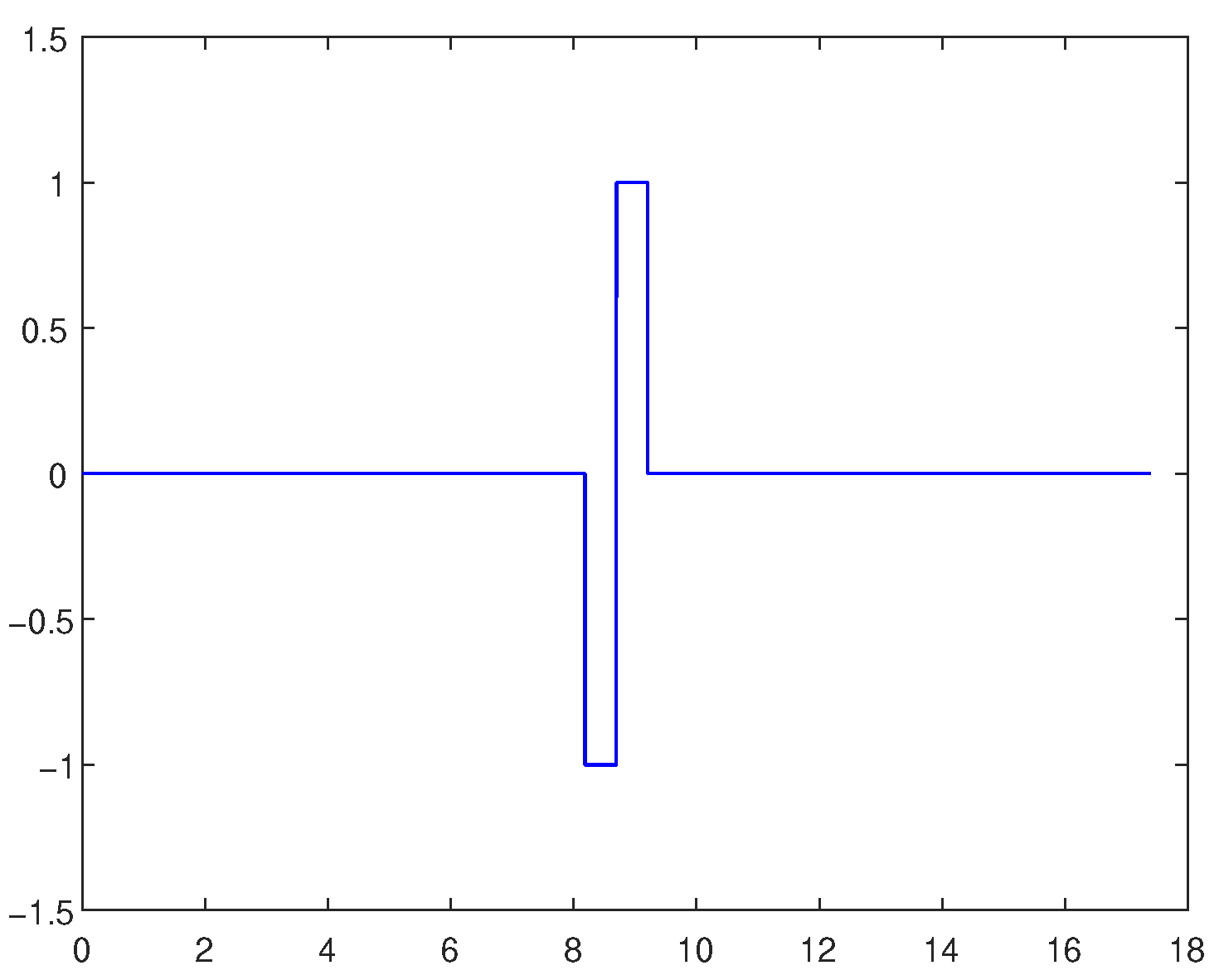
Within this framework, the Haar wavelet (Figure 1) is the minimal orthonormal case with $L=2$,

$$h_0=h_1={\displaystyle \frac{1}{\sqrt{2}}},g_0={\displaystyle \frac{1}{\sqrt{2}}},g_1=-{\displaystyle \frac{1}{\sqrt{2}}},$$

(4)

or, equivalently, ${\varphi }_{\mathrm{H}}\left(t\right)=1$ on $[0,1)$ and zero elsewhere, while ${\psi }_{\mathrm{H}}\left(t\right)=1$ on $[0,\frac{1}{2})$, $-1$ on $[\frac{1}{2},1)$, and zero elsewhere. It has a single vanishing moment, is discontinuous, and is maximally localized in time. Consequently, it annihilates constant segments away from discontinuities and represents piecewise-constant signals with nonzero detail coefficients concentrated near jumps. In denoising, this manifests as low bias around steps and other singularities, with residual variance controlled by scale-dependent thresholding.

Daubechies wavelets $\mathrm{Db}N$ are the compactly supported orthonormal solutions of the same refinement equations with $L=2N$ taps, whose high-pass filters satisfy

$$\sum _n{g}_n{n}^k=0,k=0,1,\dots ,N-1,$$

(5)

and equivalently,

$${\int }_{\mathbb{R}}{t}^k{\psi }_{\mathrm{Db}N}\left(t\right)dt=0,k=0,1,\dots ,N-1.$$

(6)

Increasing N therefore increases both support and regularity. In the present basis set, Db3 and Db9 represent intermediate- and high-regularity cases, respectively. The smoother Db9 basis functions have more vanishing moments and are very efficient for approximating $C^s$ signals without edges, thereby promoting coefficient sparsity at fine scales. The trade-off is that their longer support tends to straddle discontinuities, distributing an edge across multiple neighboring coefficients and potentially inducing pseudo-Gibbs oscillations if thresholding is applied naively near jumps [3,15].

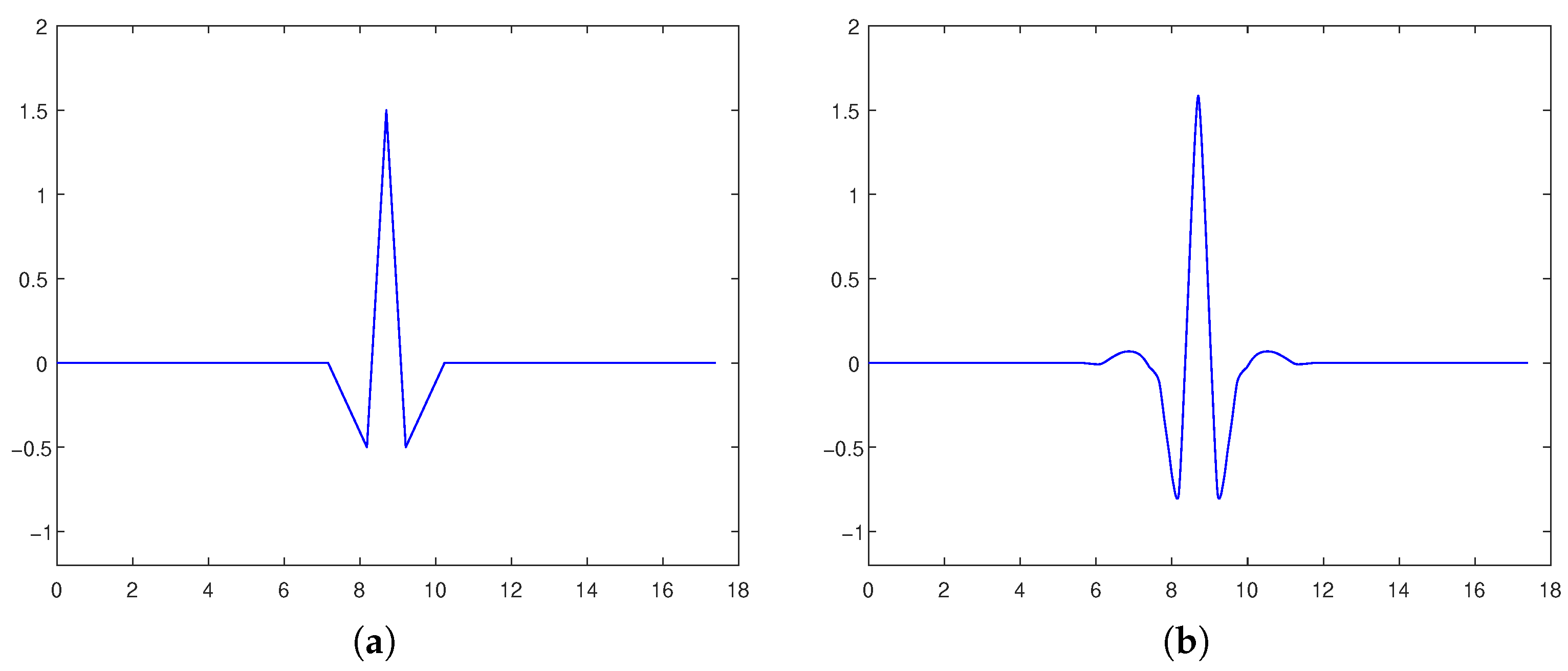
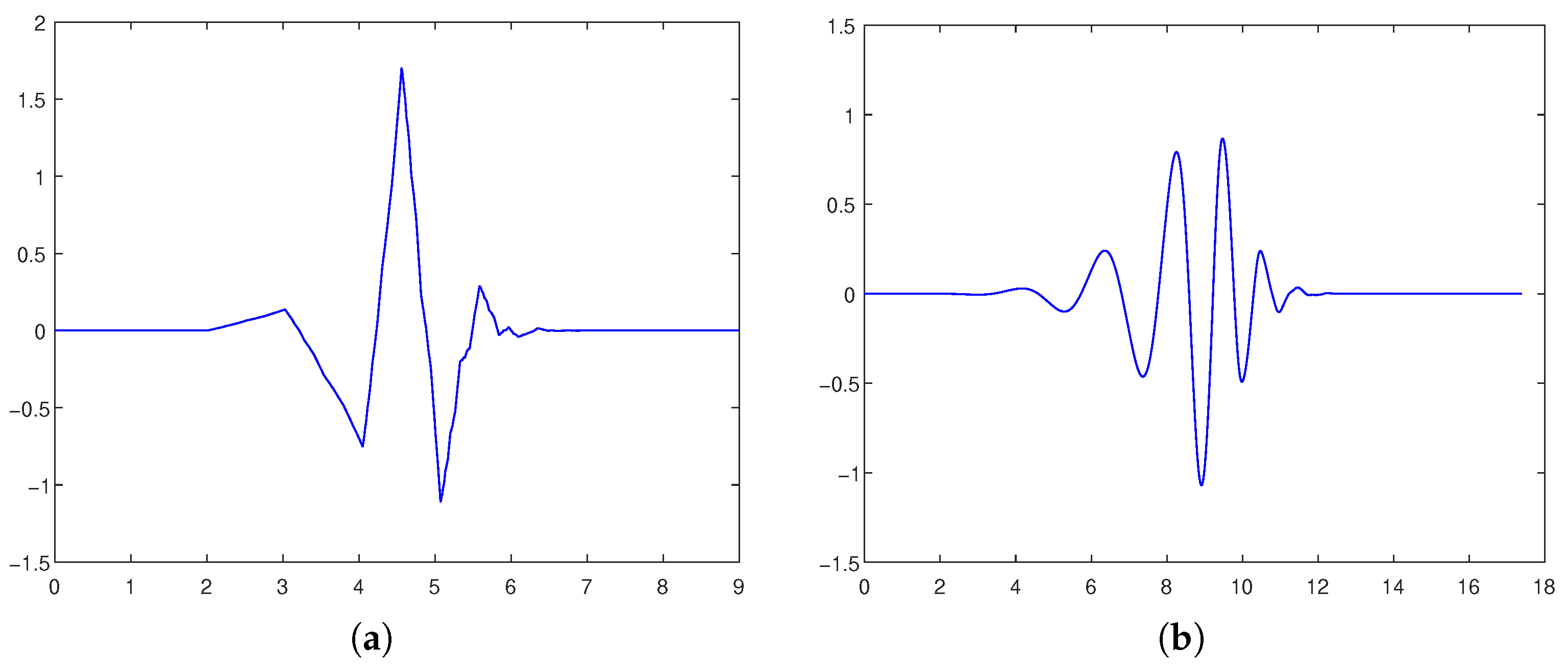
Figure 2a shows Db3, the intermediate-order representative of the orthonormal Daubechies family used in the experiments. In the refinement description above, it corresponds to $N=3$, i.e., a six-tap filter with three vanishing moments. Its scaling and wavelet functions are continuous but not continuously differentiable, making it a useful compromise for signals that contain both smooth segments and sharp transitions, such as Bumps or HeaviSine.

Between these orthonormal extremes, we also investigate the Bior family of compactly supported biorthogonal spline wavelets [13,16]. Instead of a single orthonormal pair $(\varphi ,\psi )$, this family uses primal and dual scaling functions and wavelets, $(\varphi ,\psi )$ and $(\tilde{\varphi },\tilde{\psi })$, satisfying

$$\varphi \left(t\right)=\sqrt{2}\sum _n{h}_n\varphi (2t-n),\tilde{\varphi }\left(t\right)=\sqrt{2}\sum _n{\tilde{h}}_n\tilde{\varphi }(2t-n),$$

(7)

$$\psi \left(t\right)=\sqrt{2}\sum _n{g}_n\varphi (2t-n),\tilde{\psi }\left(t\right)=\sqrt{2}\sum _n{\tilde{g}}_n\tilde{\varphi }(2t-n),$$

(8)

with biorthogonality conditions $\langle \varphi (·-k),\tilde{\varphi }(·-\ell )\rangle ={\delta }_{k\ell }$ and $\langle \psi (·-k),\tilde{\psi }(·-\ell )\rangle ={\delta }_{k\ell }$. This relaxes strict orthonormality and allows symmetric or near-symmetric filters with linear phase and exact reconstruction, while retaining compact support and explicit control of primal/dual vanishing moments. We use Bior2.2 and Bior4.4, whose primal and dual wavelets each provide two and four vanishing moments, respectively, as shown in Figure 3.

These qualitative behaviors align with the canonical nonparametric risk theory for wavelet shrinkage. For signals that are globally smooth (e.g., belonging to Besov spaces with large s), longer and smoother wavelets reduce approximation error at fixed resolution, and thresholded reconstructions display a lower MSE away from boundaries. For signals that are only piecewise smooth with isolated singularities, the bias from oversmoothing near edges can dominate unless the basis is sufficiently localized. In particular, short-support wavelets (Haar, low-order Daubechies or symmlets) better confine the effect of a jump to a small neighborhood in the coefficient domain, improving edge fidelity after shrinkage [2,15]. Although translation-invariant shrinkage could be used to further mitigate artifacts due to downsampling and phase alignment, the edge-localization advantage of shorter wavelets remains fundamental [3].

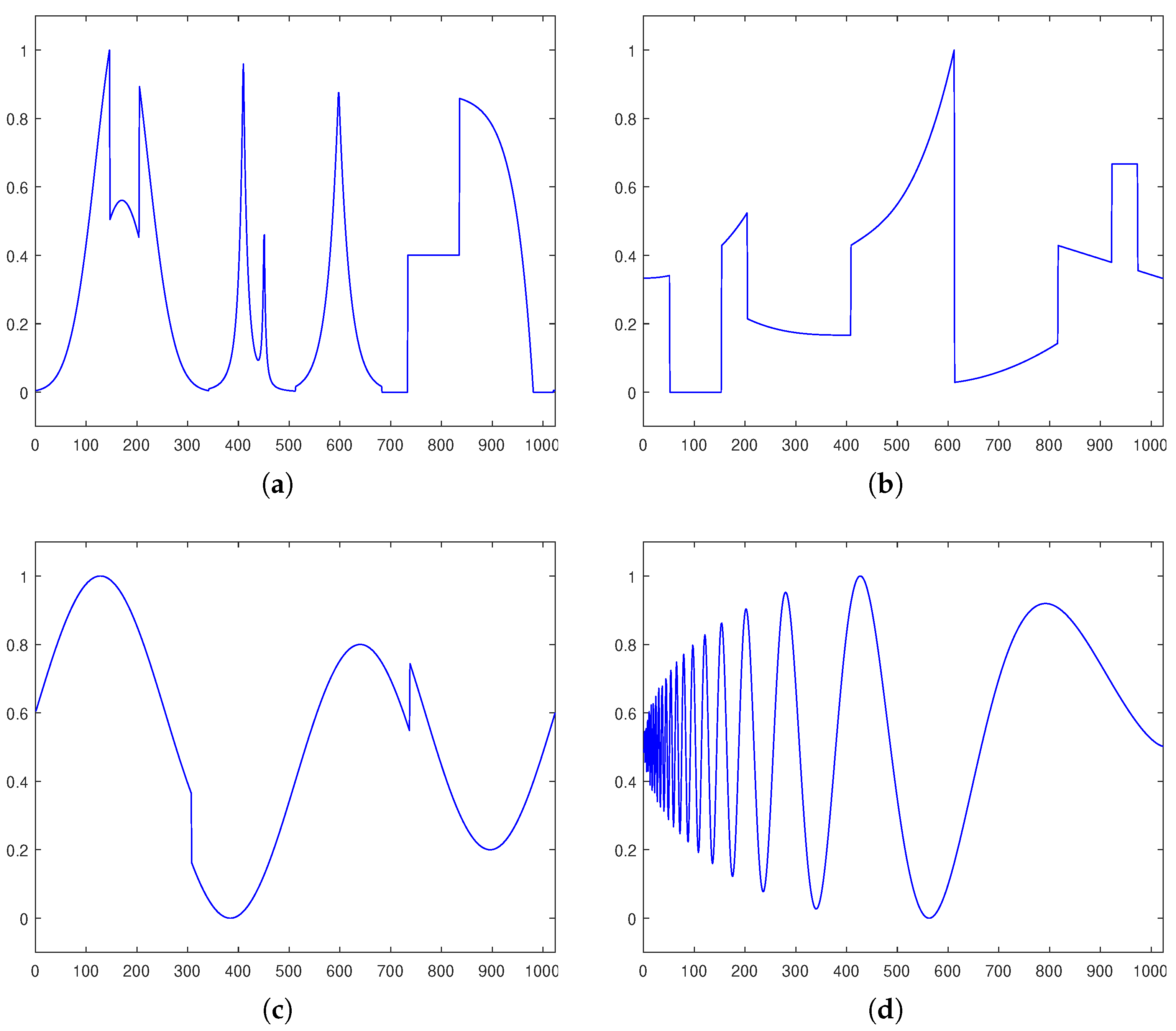
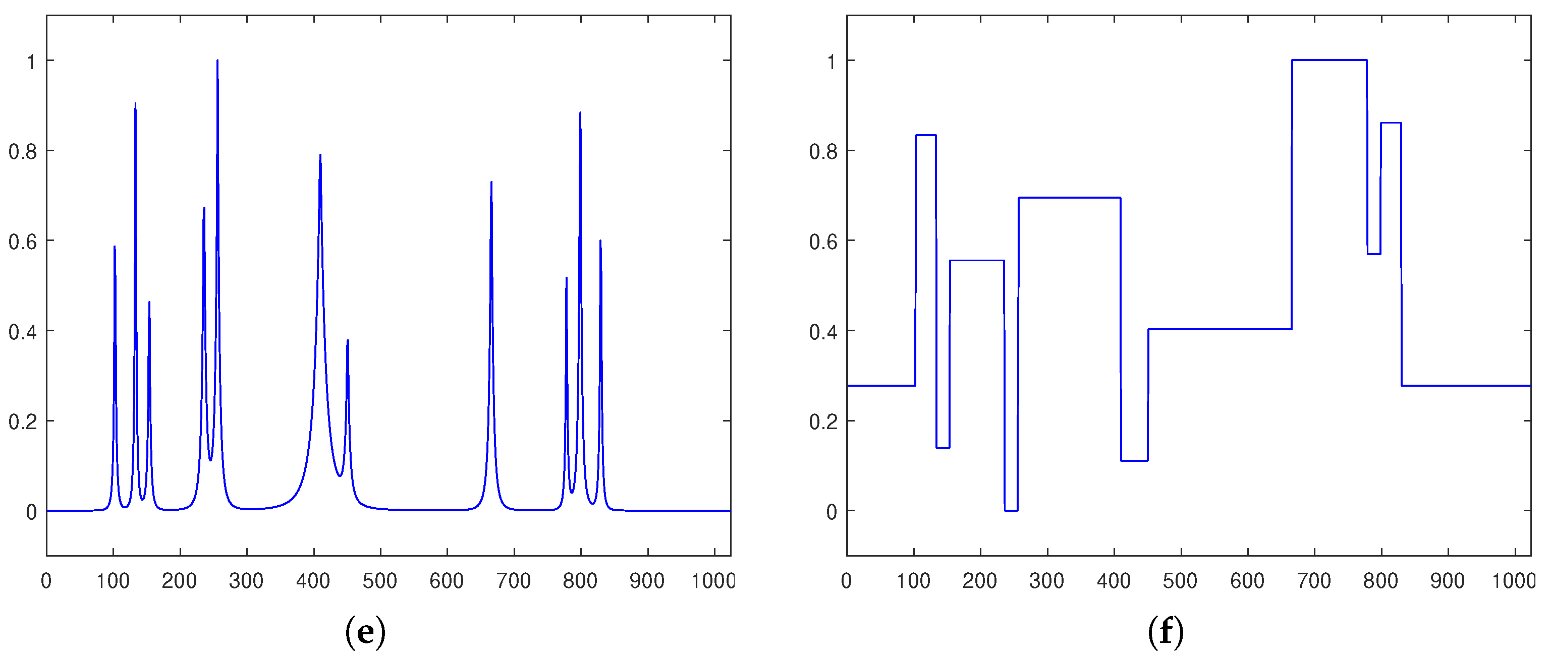
The practical implications of this design choice are evident when considering standard test signals (Figure 4). Blocks and, to a lesser extent, HeaviSine exhibit jump discontinuities; short-support wavelets (e.g., Haar) provide parsimonious representations that preserve edges with minimal ringing after thresholding. Bumps contains localized high-frequency features on a relatively smooth background. Short-to-intermediate support wavelets capture the narrow peaks without excessive spatial smearing. Doppler displays spatially varying smoothness and oscillation frequency. Bases of intermediate length often balance time–frequency localization and smooth-region sparsity. In contrast, Piece-polynomial and Piece-regular are dominated by smooth segments of higher order. Longer, smoother wavelets such as Db9 (Figure 2b) yield faster coefficient decay within each smooth piece, thereby lowering the denoising risk in those regions [13,14].

In summary, there is a principled bias–variance trade-off tied to wavelet regularity and support: longer and smoother wavelet bases are preferable for globally smooth signals with no edges, due to accelerated coefficient decay and reduced approximation error. Shorter, more localized bases are preferable for signals with sharp transitions, because they confine discontinuities and limit thresholding-induced artifacts. The following sections adopt this guideline when selecting the analysis basis across the signal test suite in Figure 4, with Haar (Figure 1) and Db9 (Figure 2b) serving as representative extremes along the regularity–support spectrum.

3. Distribution of Wavelet Coefficients

A discrete wavelet decomposition produces, at every level, two complementary subbands: a low-pass (approximation) part and a high-pass (detail) part. The low-pass branch captures the local average of the signal and therefore represents a coarse-scale approximation, whereas the high-pass branch collects the rapidly varying components and fine structure. Under a stochastic signal model, the detail coefficients at a fixed level are treated as realizations of a weakly dependent within-scale process. The PDF referred to below is the marginal distribution of that process, estimated empirically from the observed subband coefficients.

We assume that the observed signal $z\left(x\right)$ is a noisy measurement of an underlying clean signal $y\left(x\right)$:

$$z\left(x\right)=y\left(x\right)+\epsilon \left(x\right),$$

(9)

where $\epsilon \left(x\right)$ is additive noise.

A corresponding decomposition applies at the level of coefficient statistics. Because the transform is linear,

$$\mathcal{W}\left(z\right(x\left)\right)=\mathcal{W}\left(y\right(x\left)\right)+\mathcal{W}\left(\epsilon \right(x\left)\right).$$

(10)

If $d_{j,k}^{\left(z\right)}=\langle z,{\psi }_{j,k}\rangle$ denotes the detail coefficient at scale j and location k, then

$$\begin{array}{cc}\hfill d_{j,k}^{\left(z\right)}& =\langle z,{\psi }_{j,k}\rangle \hfill \\ \hfill & =\langle y,{\psi }_{j,k}\rangle +\langle \epsilon ,{\psi }_{j,k}\rangle \hfill \\ \hfill & =d_{j,k}^{\left(y\right)}+d_{j,k}^{\left(\epsilon \right)}.\hfill \end{array}$$

(11)

Under the usual independence assumption between signal and noise, the corresponding coefficient PDFs satisfy the convolution identity

$$\begin{array}{cc}\hfill p_{d_{j,k}^{\left(z\right)}}\left(u\right)& =(p_{d_{j,k}^{\left(y\right)}}\ast p_{d_{j,k}^{\left(\epsilon \right)}})\left(u\right),\hfill \\ \hfill {\phi }_{d_{j,k}^{\left(z\right)}}\left(t\right)& ={\phi }_{d_{j,k}^{\left(y\right)}}\left(t\right){\phi }_{d_{j,k}^{\left(\epsilon \right)}}\left(t\right),\hfill \end{array}$$

(12)

where $\phi$ denotes the characteristic function. In particular,

$$Var\left(d_{j,k}^{\left(z\right)}\right)=Var\left(d_{j,k}^{\left(y\right)}\right)+Var\left(d_{j,k}^{\left(\epsilon \right)}\right).$$

(13)

Hence, the observed coefficient PDF is a noise-broadened version of the clean-signal coefficient PDF, and the amount of broadening is determined by the wavelet-domain noise energy at the given scale. This decomposition underlies the scale and noise analyses below.

3.1. Impact of Scale

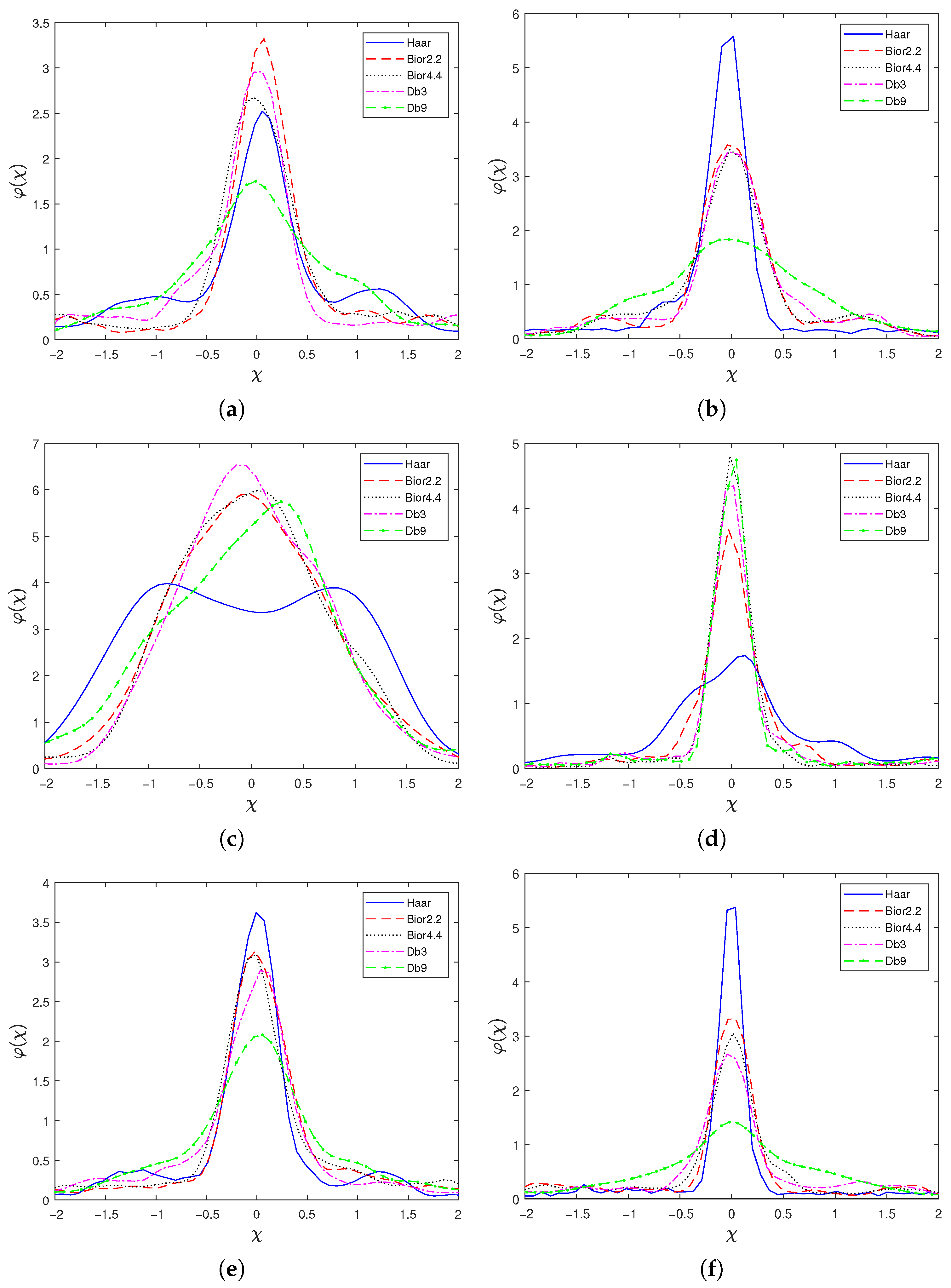
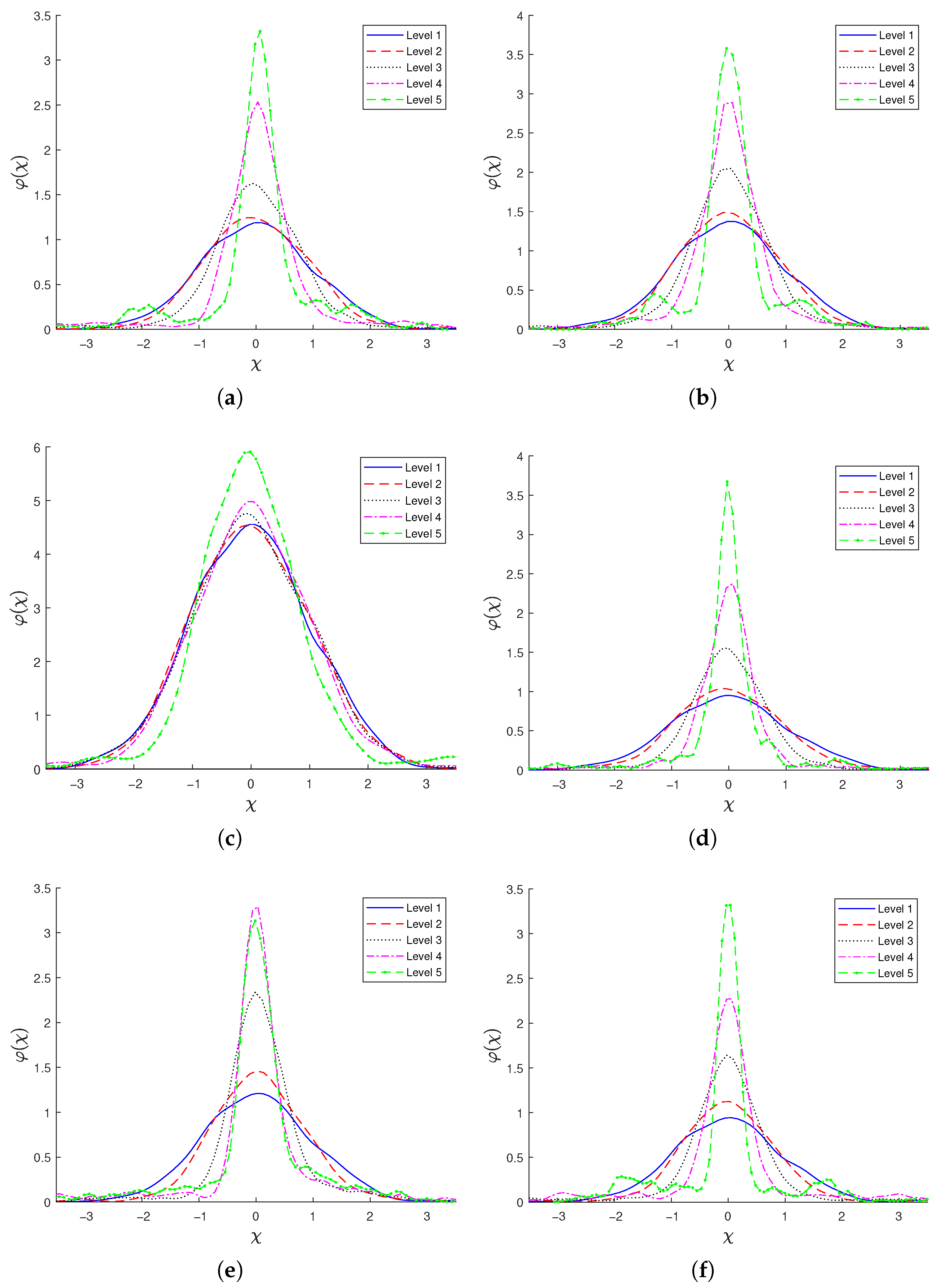
Figure 5 illustrates how the coefficient PDF evolves across five decomposition levels for several test signals, using Bior2.2 as the analysis wavelet. A consistent trend is visible: at the first level the empirical PDF is typically close to a Gaussian, whereas deeper levels yield progressively tighter distributions with a sharper peak around zero. Two signals show slight departures from the monotone behavior. For Bumps in Figure 5e, the level-4 PDF has a marginally higher peak than the level-5 PDF, and for HeaviSine in Figure 5c, the separation between levels is less pronounced than in other examples. These differences are attributable to additional interacting factors discussed later.

This scale-dependent behavior is consistent with the present benchmark class. The considered test signals are dominated by low-frequency content, so coarser detail bands intercept more of the clean-signal energy than the finest high-pass band. Let

$$E_j^{\left(y\right)}=\sum _k{\left|d_{j,k}^{\left(y\right)}\right|}^2$$

denote the clean-signal energy in detail subband j. By Parseval’s identity,

$$E_j^{\left(y\right)}={\int }_{\mathbb{R}}{\left|{\Psi }_j\left(f\right)\right|}^2{\left|\widehat{y}\left(f\right)\right|}^{2}df,$$

where ${\Psi }_j$ is the level-j detail response. Under the present scale convention, a larger j corresponds to a lower center frequency. Hence, for signals whose energy is concentrated at low frequencies, $E_j^{\left(y\right)}$ typically increases as j moves toward coarser detail levels [4]. By contrast, for additive white Gaussian noise and an orthonormal DWT, the noise variance per coefficient is approximately scale-invariant up to finite-length and boundary effects [2,4]. The relative signal contribution in the detail coefficients therefore increases toward coarser levels. This explains why first-level coefficients in the present experiments often look approximately Gaussian, whereas deeper levels exhibit the sharper central concentration associated with sparse signal representations.

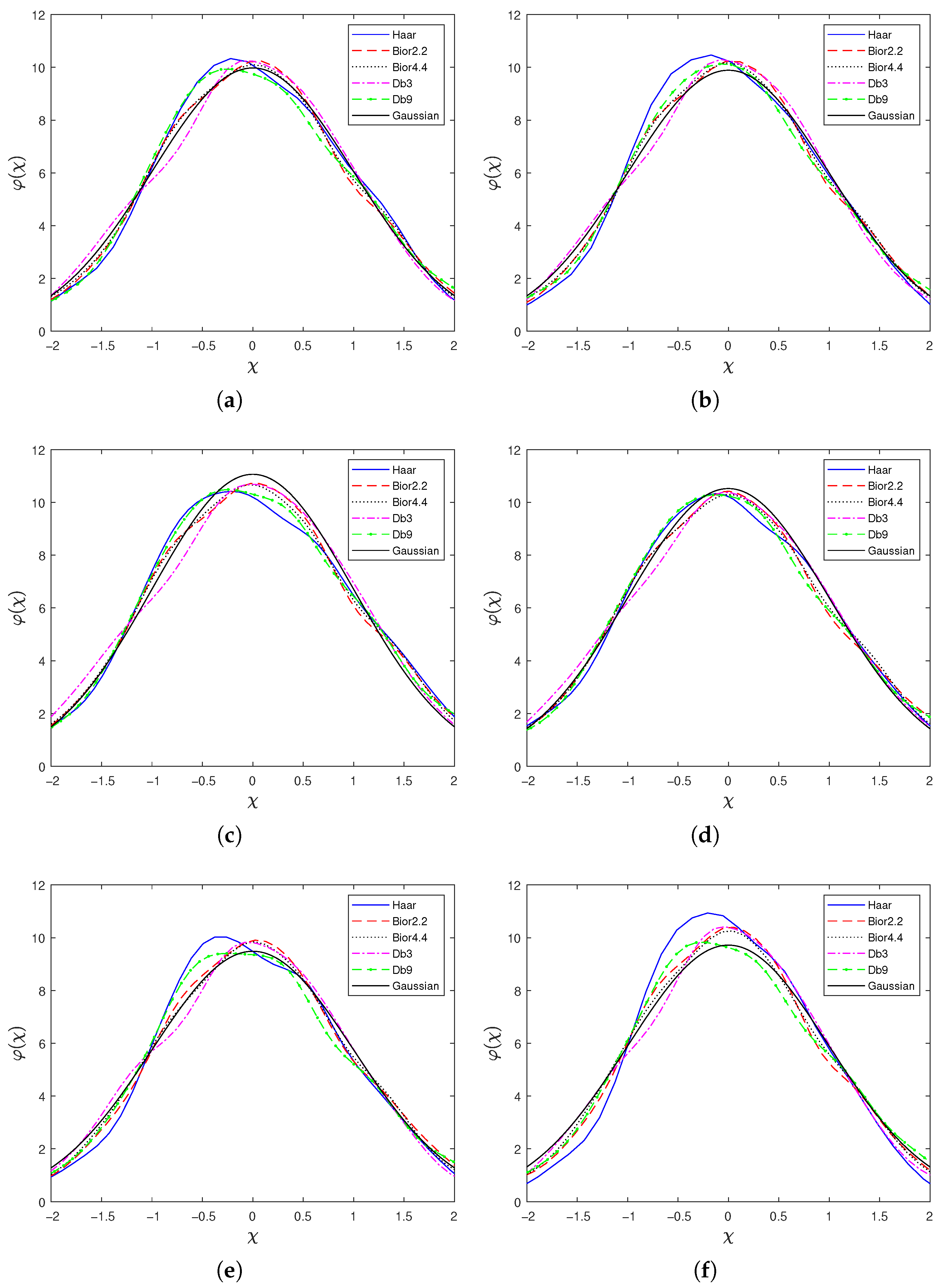
This is corroborated in Figure 6, which compares first-level coefficient PDFs for multiple wavelet bases (and includes a Gaussian PDF for reference). At this initial level, changing either the wavelet basis or the particular test signal has only a minor effect in the present experiments: most coefficient PDFs remain close to Gaussian. Hence, for level 1, it is difficult to associate the coefficient PDF shape with the suitability of a wavelet basis for a given signal.

As the decomposition proceeds, the high-pass channel corresponds to increasingly narrower bands at lower frequencies. At these coarser scales, the noise contribution to the detail coefficients diminishes while the signal contribution becomes more prominent. Additionally, wavelet representations exhibit energy compaction: a large portion of the signal information can be captured by a relatively small number of comparatively large-magnitude coefficients. The combined effect is a sparse coefficient set whose PDF is strongly concentrated near zero, which is evident at the last decomposition level (Figure 7 and Figure 8).

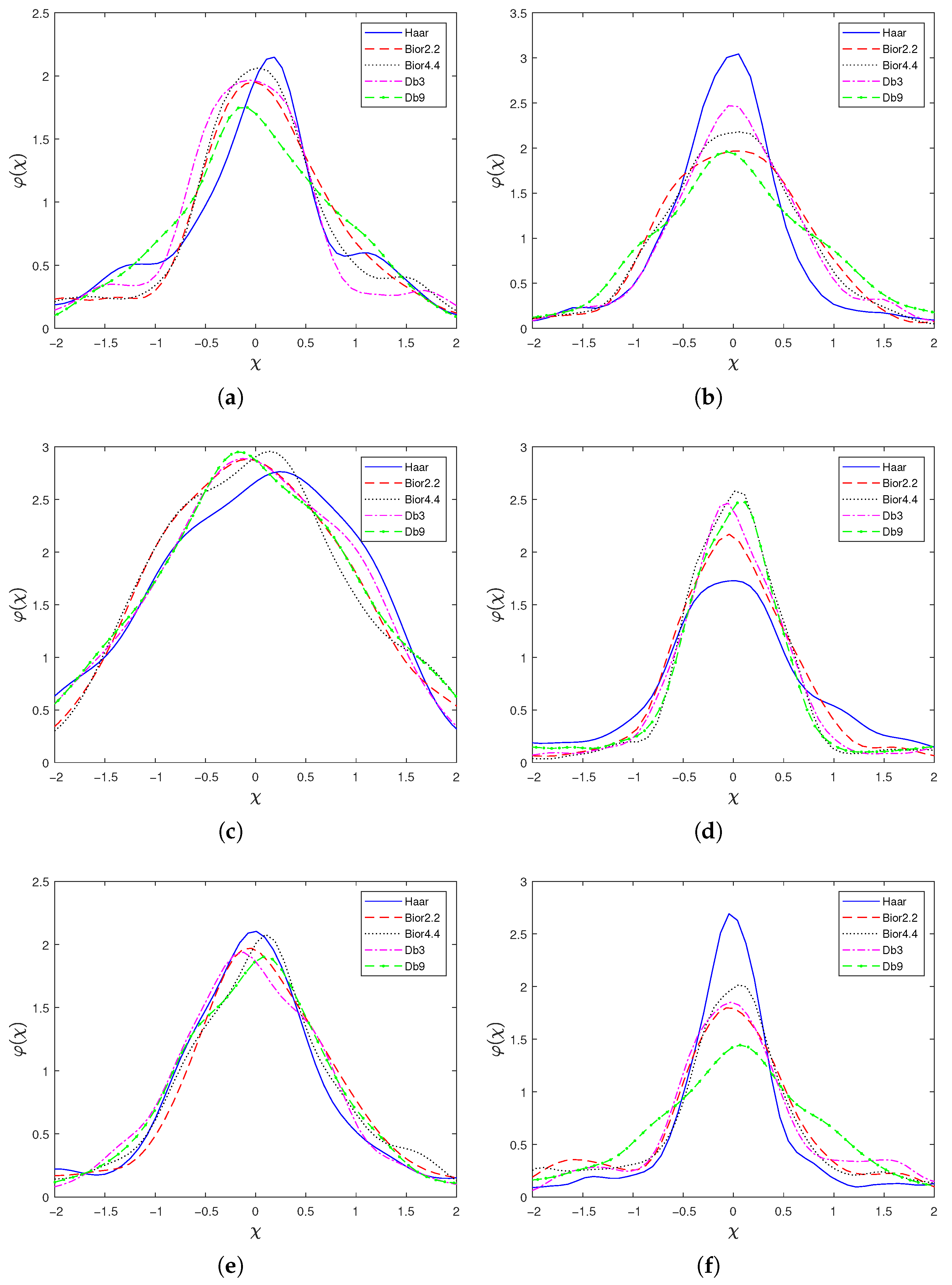
At the last level, differences between wavelet bases become pronounced. More importantly, the observed PDF shapes align with the intuition that a wavelet basis that matches local signal structure yields a sparser representation: the last-level coefficient PDF becomes narrower and more sharply peaked.

Two illustrative cases are Blocks (Figure 4f) and Doppler (Figure 4d). Because Blocks is piecewise constant and contains abrupt discontinuities, the Haar wavelet (Figure 1) provides a natural representation due to its ability to capture sharp edges efficiently. In contrast, Doppler is characterized by smoother structures and lower-frequency components, making longer and smoother wavelets more appropriate than very short bases such as Haar. As shown in the Section 4, this intuition is confirmed by the last-level coefficient PDFs: for Blocks, the Haar-based PDF is the narrowest and has the highest peak among the compared bases, whereas for Doppler, the Bior4.4 and Db9 bases produce noticeably narrower and more peaked PDFs than the other candidates.

3.2. Impact of Noise Level and Type

When the noise level is small, wavelet-domain denoising can be highly effective: with an appropriate basis, even subtle signal features can be preserved during reconstruction. As the noise variance increases, signal characteristics become progressively obscured, which degrades transform performance even if the basis is well matched to the clean signal. At a fixed level j, write ${\sigma }_{y,j}^2=Var\left(d_{j,k}^{\left(y\right)}\right)$ and ${\sigma }_{\epsilon ,j}^2=Var\left(d_{j,k}^{\left(\epsilon \right)}\right)$. Then,

$$Var\left(d_{j,k}^{\left(z\right)}\right)={\sigma }_{y,j}^2+{\sigma }_{\epsilon ,j}^2.$$

(14)

If ${\kappa }_{4,j}^{\left(y\right)}$ and ${\kappa }_{4,j}^{\left(\epsilon \right)}$ denote the fourth cumulants, the excess kurtosis of the observed coefficient is

$${\gamma }_{2,j}^{\left(z\right)}={\displaystyle \frac{{\kappa }_{4,j}^{\left(y\right)}+{\kappa }_{4,j}^{\left(\epsilon \right)}}{{\left({\sigma }_{y,j}^2+{\sigma }_{\epsilon ,j}^2\right)}^2}}.$$

(15)

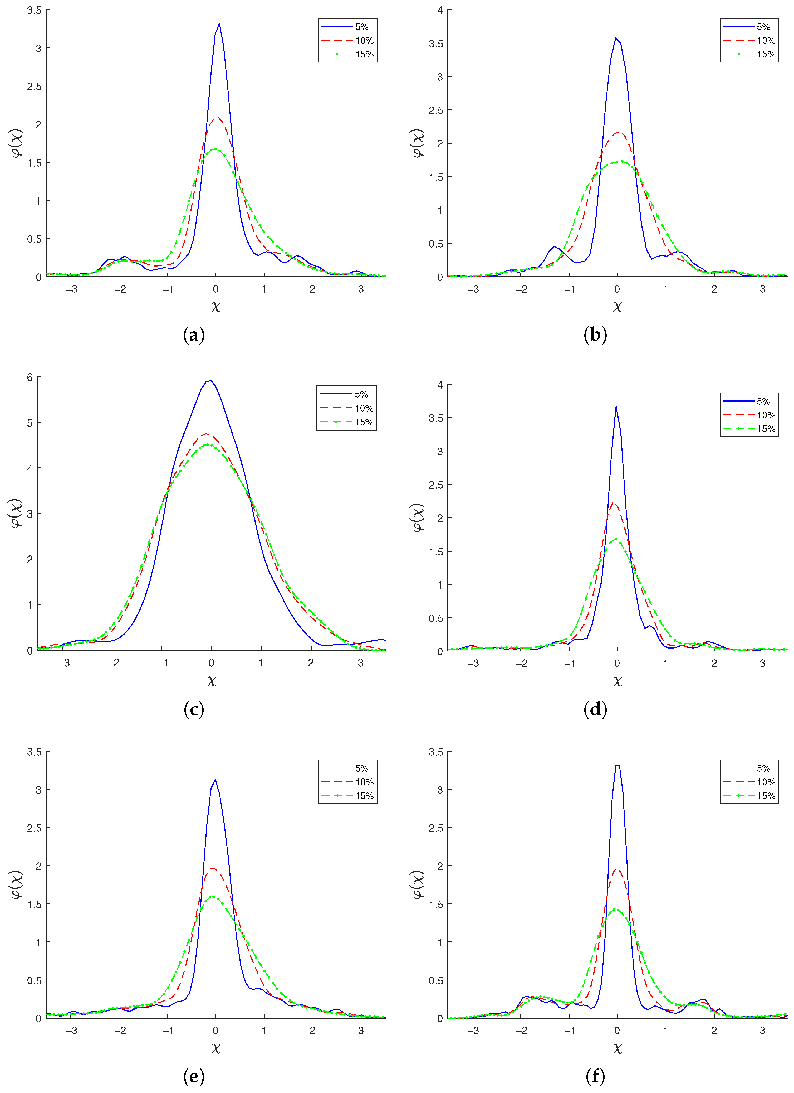
Thus, increasing the noise variance enlarges the denominator and reduces the standardized peakedness of the observed coefficient distribution. Under the proposed hypothesis, the same trend should be visible empirically in the last-level coefficient PDF, and Figure 7 confirms that this is the case for all test signals. For each signal, the most suitable wavelet basis was selected from among three candidates. Additive white Gaussian noise with ${\sigma }_{\epsilon }\in \{5\%,10\%,15\%\}$ of the signal magnitude was applied. Although multiple factors influence the empirical PDF and the magnitude of the effect differs between signals, higher noise levels consistently lead to less leptokurtic last-level coefficient distributions.

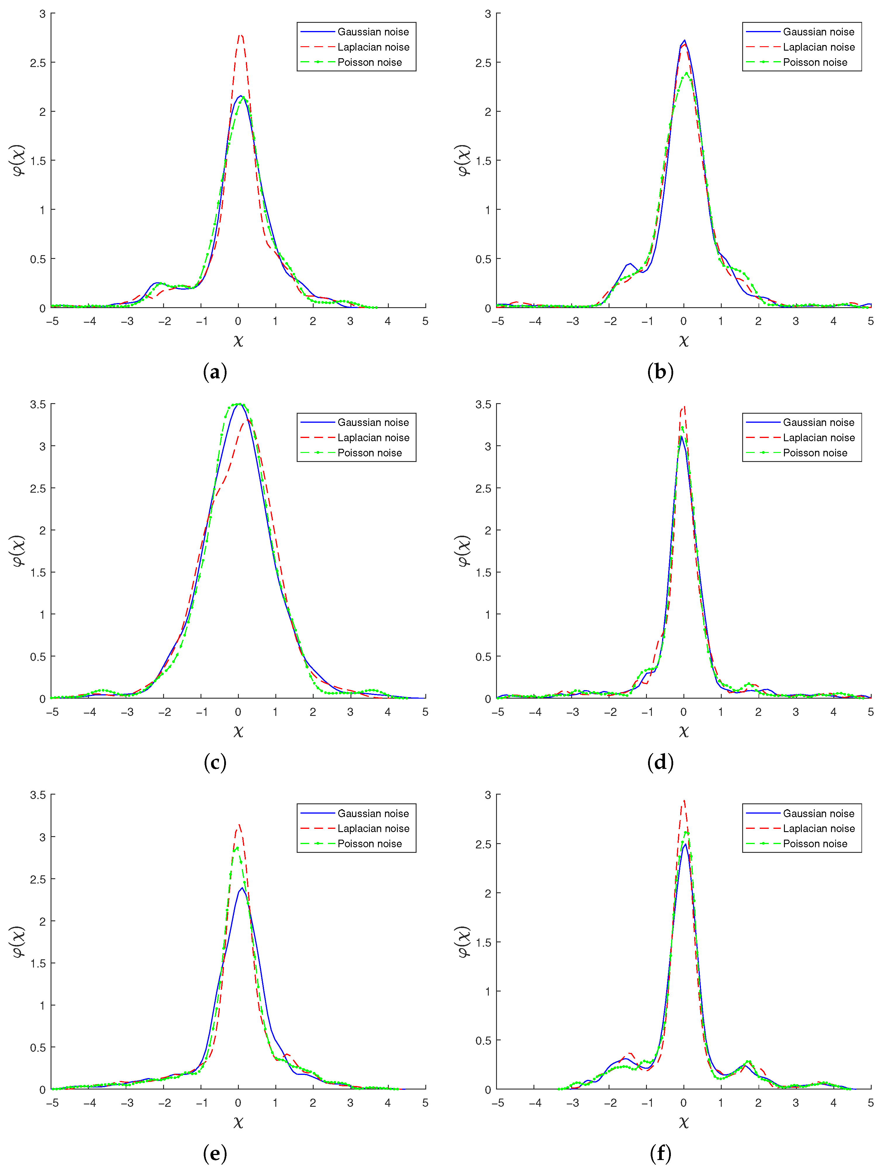
Figure 8 provides an empirical comparison across noise models. The test signals were corrupted with Gaussian, Poisson, and Laplacian noise, each normalized to the same nominal level ${\sigma }_{\epsilon }=10\%$ of the signal magnitude, and the resulting last-level coefficient PDFs are, in general, very similar across these cases.

4. Results and Discussion

To test the proposed hypothesis, we performed wavelet-shrinkage denoising of each test signal (Figure 4) using each of the investigated wavelet bases. We conducted two experiments: one with additive white Gaussian noise of level ${\sigma }_{\epsilon }=5\%$ of the signal magnitude, and another with ${\sigma }_{\epsilon }=15\%$. We then evaluated performance objectively via the root-mean-square error (RMSE) and identified, for each signal, the best-performing wavelet basis. This basis choice was compared to the selection predicted by the wavelet-coefficient PDF shape analysis.

We used standard wavelet shrinkage; let the observed samples be:

$$z_i=f\left(t_i\right)+{\epsilon }_i,i=0,\dots ,N-1,$$

(16)

with independent noise terms ${\epsilon }_i\sim \mathcal{N}(0,{\sigma }_{\epsilon }^2)$. Applying a discrete wavelet transform (DWT) with analysis functions $\tilde{\psi }$ and $\tilde{\varphi }$ yields detail (w) and approximation (a) coefficients:

$$\begin{array}{c}\hfill w_{j,k}=\langle z,{\tilde{\psi }}_{j,k}\rangle ,{\tilde{\psi }}_{j,k}\left(t\right)=2^{-j/2}\tilde{\psi }(2^{-j}t-k),\\ \hfill a_{j,k}=\langle z,{\tilde{\varphi }}_{j,k}\rangle ,{\tilde{\varphi }}_{j,k}\left(t\right)=2^{-j/2}\tilde{\varphi }(2^{-j}t-k).\end{array}$$

(17)

For orthonormal wavelet bases, $\tilde{\psi }=\psi$ and $\tilde{\varphi }=\varphi$; for biorthogonal wavelets, $(\tilde{\varphi },\tilde{\psi })$ denote the analysis pair and $(\varphi ,\psi )$ the synthesis pair.

For an orthonormal DWT, white Gaussian noise remains Gaussian with equal variance across coefficients up to finite-length and boundary effects. For biorthogonal transforms, coefficient noise is generally correlated and may be level-dependent, although coefficient-wise thresholding remains standard practice [2,4]. The hard thresholding used here was:

$${\widehat{w}}_{j,k}={\mathcal{H}}_{\lambda }\left(w_{j,k}\right)=w_{j,k}\mathbf{1}\left(|w_{j,k}|\ge \lambda \right),$$

(18)

where $\mathbf{1}\left(|w_{j,k}|\ge \lambda \right)$ is the indicator function:

$$\mathbf{1}\left(|w_{j,k}|\ge \lambda \right)=\left\{\begin{array}{cc}1,\hfill & |w_{j,k}|\ge \lambda ,\hfill \\ 0,\hfill & |w_{j,k}|<\lambda .\hfill \end{array}\right.$$

(19)

The denoised signal was then obtained from the inverse DWT,

$$\widehat{f}\left(t_i\right)=\sum _k{a}_{J_0,k}{\varphi }_{J_0,k}\left(t_i\right)+\sum _{j=1}^{J_0}\sum _k{\widehat{w}}_{j,k}{\psi }_{j,k}\left(t_i\right),$$

(20)

where $J_0$ is the coarsest scale level.

Within this benchmark setup, the total number of decomposition levels was fixed to the value that yielded the best overall reference denoising performance for the analyzed canonical signals, and the same value was used across all signals.

To isolate basis effects from threshold effects, multiple denoising runs with different thresholds were carried out and the lowest-RMSE threshold was retained for each benchmark case. These best-case RMSE values were used only as a controlled reference and not as a practical recommendation for real-world deployment.

4.1. Denoised Signal RMSE

The RMSE values are reported in

Table 1. RMSE after denoising for signals corrupted by additive white Gaussian noise with ${\sigma }_{\epsilon }=5\%$ of the signal magnitude. RMSE is scaled by ${10}^2$.

Signal	Haar	Bior2.2	Bior4.4	Db3	Db9
Piece-Regular	1.73	1.75	1.80	1.72	2.32
Piece-Polynomial	1.21	1.79	1.85	1.84	2.47
HeaviSine	1.27	1.14	1.18	1.18	1.41
Doppler	2.49	1.84	1.66	1.76	1.71
Bumps	1.99	1.91	1.99	2.03	2.53
Blocks	1.22	1.86	2.01	1.99	2.70

Note: Boldface indicates the best-performing result for each signal.

and

Table 2. RMSE after denoising for signals corrupted by additive white Gaussian noise with ${\sigma }_{\epsilon }=15\%$ of the signal magnitude. RMSE is scaled by ${10}^2$.

Signal	Haar	Bior2.2	Bior4.4	Db3	Db9
Piece-Regular	4.50	4.61	5.00	4.84	5.63
Piece-Polynomial	3.71	4.69	4.97	4.80	5.53
HeaviSine	2.58	2.77	2.87	2.83	2.93
Doppler	5.57	4.62	4.43	4.66	4.79
Bumps	5.71	5.21	5.61	5.53	6.36
Blocks	4.09	5.39	5.70	5.69	6.54

Note: Boldface indicates the best-performing result for each signal.

. For signals dominated by discontinuities or low-order polynomials (Blocks and Piece-Polynomial), the shortest and least smooth wavelet, Haar, achieves the smallest error at both noise levels (${\sigma }_{\epsilon }=5\%$ and $15\%$ of the signal magnitude). For example, for Blocks at $5\%$ noise, Haar attains an RMSE of $1.22\times {10}^{-2}$, compared with $1.86\times {10}^{-2}$ for Bior2.2 and even larger errors for the smoother wavelets; a similar margin is observed at $15\%$ noise. This is consistent with the interpretation of the Haar wavelet as a localized step function: it can represent piecewise-constant or piecewise-polynomial structure with very few significant coefficients and minimal ringing near jump discontinuities, while smoother wavelets tend to overshoot and smear edges.

In contrast, for the smooth, highly non-stationary Doppler signal, longer and smoother wavelets with more vanishing moments provide a clear advantage. Bior4.4, with four vanishing moments and good regularity, yields the lowest RMSE at both noise levels ($1.66\times {10}^{-2}$ and $4.43\times {10}^{-2}$ for $5\%$ and $15\%$ noise, respectively), with Db9 a close second. Compared to Haar, this corresponds to a reduction of roughly $30\%$ at the lower noise level and about $20\%$ at the higher noise level. The Doppler waveform is well approximated locally by low-degree polynomials, so wavelets with several vanishing moments produce very sparse representations in smooth regions; after thresholding, most remaining coefficients correspond to genuine oscillatory structure rather than noise, which explains the improved denoising performance.

The mixed-regularity test functions (Bumps, HeaviSine, Piece-Regular) highlight the need to balance support length and smoothness. For Bumps, consisting of smooth but sharply localized peaks, Bior2.2 consistently gives the best RMSE across both noise levels, suggesting that two vanishing moments with relatively short support offer an effective compromise between capturing smooth structure and avoiding excessive spreading of the narrow features. For HeaviSine at $5\%$ noise, Bior2.2 again performs best, whereas at $15\%$ noise the advantage shifts slightly to Haar. A plausible explanation is that at higher noise levels the dominant error source becomes the accurate localization of the jump discontinuities; the extra smoothness of biorthogonal and Daubechies wavelets then tends to blur the step edges under thresholding, whereas Haar preserves them more faithfully. A similar pattern is observed for the Piece-Regular signal, where Db3 (moderate smoothness and support) is best at $5\%$ noise, but Haar becomes optimal when the noise level increases.

Averaging over the three “smooth” benchmark signals (Bumps, Doppler, HeaviSine), the mean RMSE is lowest for Bior2.2 and Bior4.4 at both noise levels, indicating a systematic benefit of using smoother wavelets with multiple vanishing moments when the underlying signal is predominantly smooth. Conversely, averaging over the more discontinuous signals (Blocks, Piece-Polynomial, Piece-Regular) shows Haar outperforming the other families by roughly 15–$20\%$ in RMSE. Overall, the results are in line with standard wavelet approximation theory: wavelets with longer support and more vanishing moments are particularly suitable for denoising smooth, oscillatory signals such as Doppler-type waveforms, while short, less regular wavelets like Haar remain preferable for strongly piecewise-constant or piecewise-polynomial signals with many sharp transitions.

4.2. PDF Shape Based Wavelet Selection

Wavelet coefficient PDFs’ shapes are shown in Figure 9 and Figure 10, for ${\sigma }_{\epsilon }=5\%$ and ${\sigma }_{\epsilon }=15\%$ of signal magnitude, respectively. It can be seen that when ${\sigma }_{\epsilon }=5\%$, there is a distinct difference for most wavelets and test cases, while in the case of ${\sigma }_{\epsilon }=15\%$, on several test signals, the difference is less obvious. The reasons are two-fold. Firstly, some test signals contain different artifacts such that different wavelet basis perform similarly, as seen in Table 1 and Table 2. Secondly, there is the impact of noise. At extreme noise levels (${\sigma }_{\epsilon }=15\%$), some edge artifacts or fine details are inevitably obscured by the noise and are lost or poorly preserved in the reconstructed signal. As such, different wavelet bases perform similarly in terms of RMSE, but differently in terms of subjective visual quality.

To compare the denoising efficiency of the PDF-shape-based wavelet-basis selection with the other tested bases, for each test case we selected the wavelet basis that yielded the most leptokurtic PDF.

Table 3. Relative RMSE scores of PDF-shape-based selected basis and the worst-case basis, compared to the best-performing basis.

	${\mathit{\sigma }}_{\mathit{\epsilon }}=5\%$		${\mathit{\sigma }}_{\mathit{\epsilon }}=15\%$
Signal	PDF	Worst	PDF	Worst
Piece-Regular	1.02	1.35	1	1.25
Piece-Polynomial	1	2.04	1	1.49
HeaviSine	1.04	1.24	1.11	1.14
Doppler	1	1.50	1	1.26
Bumps	1.04	1.32	1.10	1.22
Blocks	1	2.21	1	1.60

show the relative performance of that selected basis and of the worst-performing basis, each compared to the best-performing wavelet basis. From the table, we see that the worst-performing bases can have more than twice the RMSE of the optimal basis. Our shape-based selection method performs very well for ${\sigma }_{\epsilon }=5\%$: it either selects the optimal basis or one whose RMSE is within ≤4% of the optimum.

For ${\sigma }_{\epsilon }=15\%$, the RMSE differences are smaller because the signal is more severely corrupted by noise, as discussed earlier. Nevertheless, the method still exhibits strong performance, selecting the optimal basis in four out of six test cases.

4.3. Theoretical Limits of the PDF-Based Criterion

The proposed selector is low-dimensional: for each candidate basis it needs to compress the last-level detail coefficients into a scalar description of peakedness. That parsimony is advantageous, but it also imposes theoretical limits on where the method can be expected to be decisive.

Initially, the criterion necessarily loses discriminative power in the noise-dominated regime. At a fixed scale j, the observed coefficient distribution is the convolution of the clean-signal and noise coefficient distributions, and its excess kurtosis satisfies (15). For Gaussian noise, ${\kappa }_{4,j}^{\left(\epsilon \right)}=0$, so if ${\sigma }_{\epsilon ,j}^2\gg {\sigma }_{y,j}^2$, then ${\gamma }_{2,j}^{\left(z\right)}\to 0$. Thus, as the noise variance increases, the observed coefficient distribution loses peakedness relative to the Gaussian benchmark. In the high-noise limit, the last-level PDFs associated with different bases become increasingly difficult to distinguish, so a selector based only on marginal peakedness cannot be expected to remain highly reliable. The empirical reduction in separability at ${\sigma }_{\epsilon }=15\%$ is therefore not merely a finite-sample artifact, but a direct consequence of the signal-plus-noise model.

Additionally, there is an intrinsic trade-off between scale and sample size. In a critically sampled DWT, the number of detail coefficients at level J is of order $N/2^J$. Thus, moving to coarser levels improves the subband signal-to-noise ratio for the present $1/f^{\alpha }$-type signals but simultaneously reduces the sample size available for estimating the PDF shape. Under standard regularity conditions, the sampling variability of empirical shape statistics is therefore of order $O_p\left({(N/2^J)}^{-1/2}\right)$. The last level is consequently the most informative only as long as enough coefficients remain for stable PDF-shape estimation; for short records, deep decompositions, or strongly localized phenomena, the statistic may become unstable.

Finally, the proposed criterion measures representational sparsity rather than denoising risk directly. A basis that yields the narrowest, most leptokurtic last-level PDF need not minimize every downstream loss function, because reconstruction error also depends on the threshold rule, threshold level, shrinkage bias, boundary artifacts, and the chosen performance metric. In the present study, thresholds were optimized separately to isolate the effect of basis choice; outside that controlled setting, the basis-selection problem and the threshold-selection problem are coupled. The method should therefore be viewed as a theoretically motivated compatibility diagnostic for basis screening, not as a universal substitute for end-to-end risk minimization.

5. Conclusions

The choice of wavelet basis has a decisive effect on denoising quality, and the results of this study show that the shape of the probability density function (PDF) of the high-pass detail coefficients at the last decomposition level is useful for wavelet-basis selection in one-dimensional (1-D) signals. Across the tested benchmark signals and noise levels, bases that produce narrower and more leptokurtic last-level PDFs are, in general, the bases whose regularity and support are better matched to the local smoothness of the signal and whose denoising performance is optimal or near-optimal.

In that sense, the central hypothesis of the paper is confirmed within the investigated setting: a clear relationship is established between the shape of the last-level coefficient PDF and the suitability of the wavelet basis for denoising. The proposed criterion is therefore not merely descriptive, but a practical data-driven indicator that can be used to screen and select candidate bases before or alongside shrinkage-based denoising. Its main advantage is its simplicity, since it relies only on statistics already generated by the transform and converts them into an interpretable measure of basis–signal match.

The study also clarifies the limits of this conclusion; the criterion becomes less informative in strongly noise-dominated cases, for short signals or very deep decompositions.

We conclude that the results establish PDF shape as a useful basis-selection cue for wavelet denoising, while also delimiting its scope. This is particularly relevant for adaptive denoising methods that are not tailored to a single signal class and therefore require a principled way to choose among candidate wavelet bases.

In future work, this analysis should extend from canonical synthetic examples to diverse classes of real-world engineering signals, where non-ideal noise, nonstationarity, finite-length effects, and application-specific structure may alter the coefficient statistics.