GRAPE: Grammatical Algorithms in Python for Evolution

Abstract

GRAPE is an implementation of Grammatical Evolution (GE) in DEAP, an Evolutionary Computation framework in Python, which consists of the necessary classes and functions to evolve a population of grammar-based solutions, while reporting essential measures. This tool was developed at the Bio-computing and Developmental Systems (BDS) Research Group, the birthplace of GE, as an easy to use (compared to the canonical C++ implementation, libGE) tool that inherits all the advantages of DEAP, such as selection methods, parallelism and multiple search techniques, all of which can be used with GRAPE. In this paper, we address some problems to exemplify the use of GRAPE and to perform a comparison with PonyGE2, an existing implementation of GE in Python. The results show that GRAPE has a similar performance, but is able to avail of all the extra facilities and functionality found in the DEAP framework. We further show that GRAPE enables GE to be applied to systems identification problems and we demonstrate this on two benchmark problems.

1. Introduction

Grammatical Evolution (GE) [1,2,3] is a grammar-based Evolutionary Algorithm (EA), inspired by Darwin’s theory of evolution by natural selection. The general idea consists of evolving a population of numeric strings, to which genetic operators, such as crossover and mutation can be applied. A grammar, specific to each problem, is used to transform these strings into syntactically correct solutions. These solutions are programs that are evaluated based on some metric, and the evolution occurs following the principle of survival of the fittest.

DEAP (Distributed Evolutionary Algorithms in Python) [4] is an evolutionary computation framework that provides all the necessary tools to easily implement evolutionary algorithms.

This paper presents GRAPE (Grammatical Algorithms in Python for Evolution), an implementation of GE using the DEAP framework, consisting of essential classes and functions to evolve GE, as well as reporting important relevant measures. In keeping with the original spirit of DEAP, with GRAPE, we aim to provide explicit algorithms and transparent data structures.

Although GE has been publicly available for more than 20 years, many of the tools that we have already implemented on DEAP were still not available for GE. Particularly, in Section 2.2, we list the most important selection methods available on DEAP, in comparison with PonyGE2, another implementation of GE in Python [5], and the difference in quantity is clear. Then, we believe that implementing GE with DEAP can attract more users to the GE community due to its ease of use and its large number of functions already implemented. Moreover, we believe that many GE researchers are already familiar with the DEAP structure for evolving Genetic Algorithms or Genetic Programming, and the migration to using GRAPE will be intuitive.

2. Grammatical Evolution

GE is a grammar-based method, which fits in the family of EAs and is used to build programs [1,2,3]. The genotype of a GE individual is represented by a variable-length sequence of codons, each being equivalent to an integer number, originally defined by eight bits. This genotype is mapped into a phenotype, a more understandable representation, which can be a mathematical expression or even an entire program in practically any language.

The evolutionary process occurs at the genotypic level, which ensures that the respective phenotypes will always be syntactically correct [6]. However, the evaluation of the individuals happens at the phenotypic level, since a phenotype is a structure, which can directly be evaluated using a fitness function.

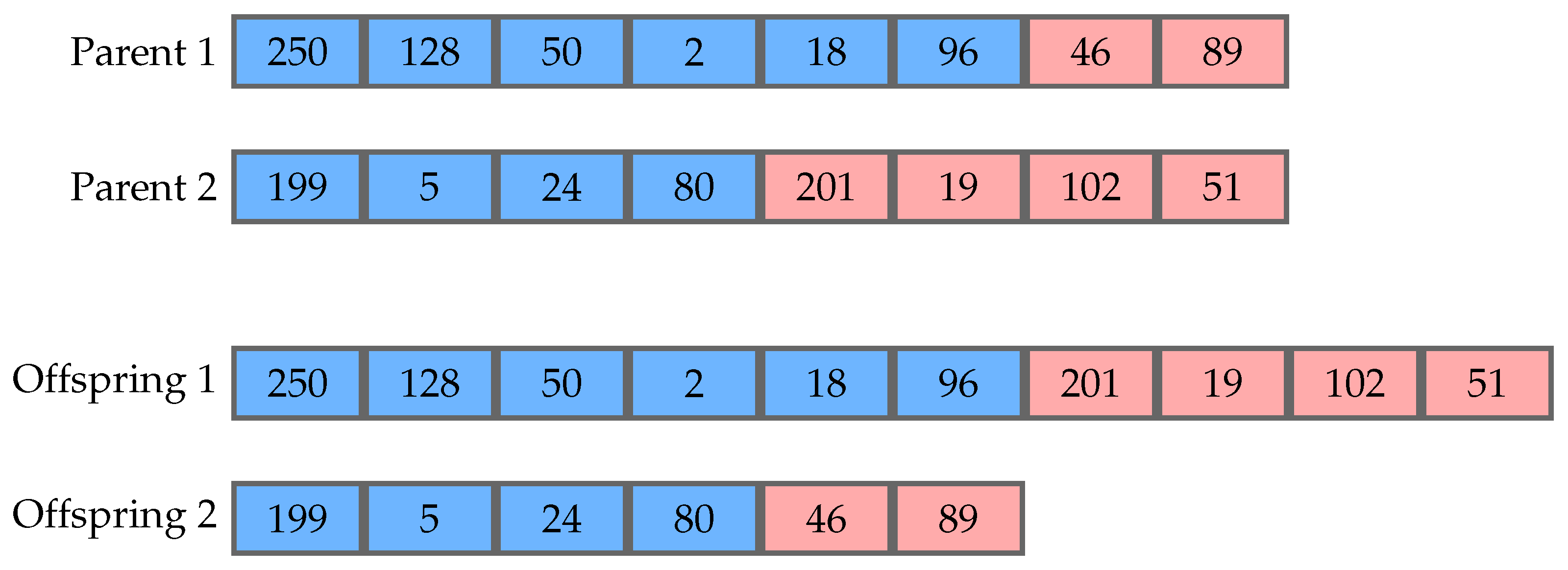
In the evolutionary process, operators such as crossover and mutation are applied to the selected parents, in order to produce new offspring for the next generation. Crossover occurs between two parents, generally generating two offspring. The most common version is one-point crossover, which consists of randomly choosing point in each parent to split them. The resulting tails are then exchanged by the parents producing the offspring. Figure 1 shows an example of this procedure. It is worth noticing that this process can change the size of the genomes. Mutation is an operator that occurs using one parent to generate one offspring and changes the value of a codon at random. In its most common version, every codon is operated on with a predefined probability, usually a small value, which avoids changing an individual too much. This operator does not change the size of a genome, but can change the size of its respective phenotype.

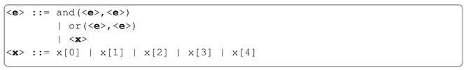
A grammar is a set of rules that define a language. In GE, grammars are usually represented in Backus-Naur Form (BNF), a notation represented by the tuple N, T, P, S, where N is the set of non-terminals, transitional structures used by the mapping process, T is the set of terminals, items that can occur in the final program, P is a set of production rules, and S is a start symbol. We can see an example of P in the Listing 1. This example represents a simple grammar with only two production rules, being the first one associated with three possible choices and the second one with five.

Listing 1. Example of production rules.

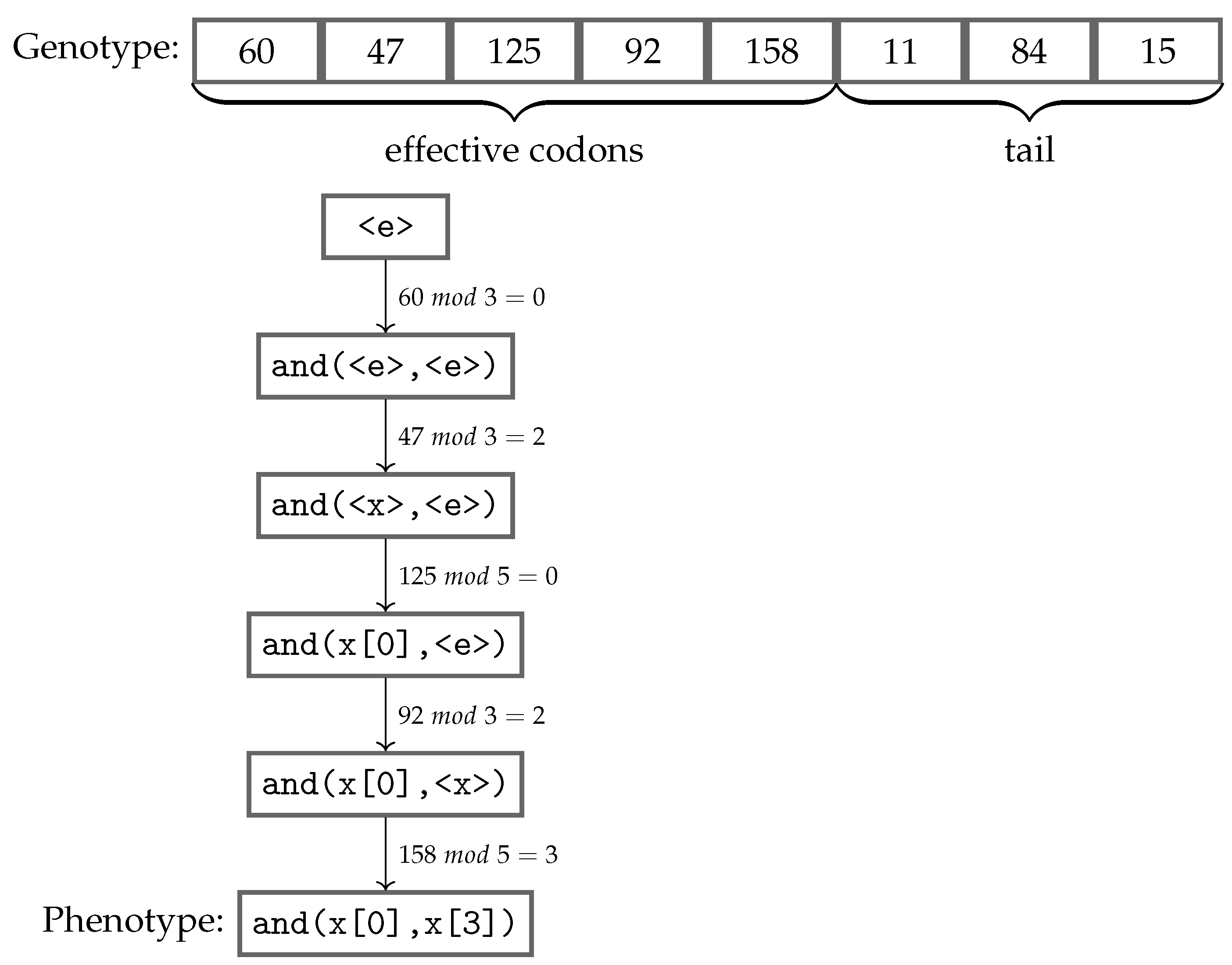
Figure 2 shows an example of the genotype-phenotype mapping process being executed using the grammar presented in Listing 1. This genotype has eight codons, and the mapping procedure starts from the leftmost one, using the modulo operator with the value of the codon and the number of possible choices in the production rule, which is being currently mapped. The choice is made according to the remainder of the division, and the process follows from left to right, always replacing the leftmost non-terminal standing in the intermediate string. Once a fully mapped phenotype, i.e., no more non-terminals, has been produced, the mapping process stops consuming codons, ignoring any remaining ones. Apart from the effective codons used in the mapping process, the unconsumed codons are named as the tail of the individual. However, if all codons were used and there are still non-terminals remaining in the phenotype, that individual is considered invalid, and usually receives the worst value possible to its fitness score. An alternative approach to reduce the possibility of an individual being considered invalid is using wrapping, which consists of reusing the codons from the beginning [6]. Nonetheless, sometimes the mapping process cannot finish even considering many wrappings.

2.1. Initialisation Methods

Random initialisation is the original method to initialise individuals in GE, which consists of generating a random value for each codon in a predefined initial genome length [1]. With this method, the initialisation process brings many invalid individuals and even a less diverse population. Moreover, depending on the grammar, the individuals tend to be short or have parse trees mostly tall and thin, which impacts on the possibilities of the population to find a good solution [7].

While random initialisation is executed at the genotypic level, other methods have explored initialisation at the phenotypic level. The full method generates individuals in which each branch has a depth equal to the predefined value for maximum initial depth, while the grow method produces individuals with different shapes that also respect the predefined maximum initial depth. The ramped half-and-half (RHH) method is a mix of the full and the grow mechanisms, and initialises GP trees with depths within the range between the predefined values for minimum initial depth and maximum initial depth [8]. Sensible initialisation is the application of RHH to GE [9], which starts by identifying which production rules are recursive, and the minimum depth necessary to finish the mapping process starting with the related non-terminal symbol for each production rule. Then, when the individuals are being initialised from the start symbol, productions are chosen in order that the individuals have depths within the range between the predefined values for minimum initial depth and maximum initial depth [10].

Another method which initialises at the phenotypic level is Position Independent Grow (PI Grow) [11], which works as the grow approach to generate derivation trees, by randomly picking production rules from the grammar. However, while expanding the branches, the next non-terminal to be replaced is randomly chosen, instead of the leftmost non-terminal as in the sensible initialisation. It allows the process to pick only recursive production rules, if the expected maximum initial depth was not achieved and there is a single non-terminal symbol remaining to map.

In both methods, sensible initialisation and PI Grow, once a phenotype is finished, the initialisation process map the sequence of necessary choices in the grammar to produce that phenotype. Then, it is possible to transform this sequence in its respective genotype. It means that we can assure that we will avoid invalid individuals in the first generation, since these methods define the phenotypes before the genotypes, unlike the random initialisation.

However, it is not a good practice to initialise genotypes having exactly the minimum number of codons to map their respective phenotypes. If we do so, the chance of producing invalid individuals when operating with crossover or mutation is higher, because the genetic material is insufficient to produce different individuals from those already existing. Then, when initialising using sensible initialisation or PI Grow, a random tail is added to each genotype, usually with 50% of the length of their effective codons, in order to reduce the propagation of invalid individuals in the following generations [12].

2.2. Selection Methods

As in most of the EAs, the selection process on GE consists of choosing individuals in the current population as parents, which will be operated by crossover, mutation etc., in order to provide offspring to the next generation. This choice is usually probabilistically based on the quality of possible parents.

One of the most known selection methods is tournament selection, in which a predefined number of individuals is chosen at random from the population and the one with the best fitness is selected as a parent. This selection is done with replacement, so the chosen parent remains in the population during the current generation, so it can be selected again.

On the other hand, lexicase selection [13] considers the fitness of each training case individually instead of an aggregated value over the whole set. Its algorithm can be seen in Listing 2, and starts with the entire population in a pool of candidates. A training case is picked at random order, and only the candidates with the best fitness value regarding that single case persist in the set of candidates. The process continues until a single candidate survives in the pool or all training cases are checked. If the first happens, that individual will be selected as a parent, and if the second happens, the choice is made randomly within the remaining candidates. This method has been tested in different kinds of problems providing successful results [14,15,16]. The reason for its success may be explained by its ability to maintain a higher level of population diversity than methods based on aggregated fitness measurements [17].

In this paper, we address problems using tournament and lexicase selection, but many other methods can be applied with GE, depending on the purpose.

Table 1. Main selection methods available in DEAP and PonyGE2.

Method	DEAP	PonyGE2
Tournament	X	X
Pareto tournament	X	X
NSGA2	X	X
NSGA3	X
Double tournament	X
Lexicase	X
Epsilon Lexicase	X

shows the main selection methods already available in DEAP (https://deap.readthedocs.io/en/master/api/tools.html accessed on 8 August 2022) and PonyGE2 (https://github.com/PonyGE/PonyGE2 accessed on 8 August 2022). Since we built GRAPE on DEAP structure, we can import these methods into our code and use them when running GE on GRAPE.

Listing 2. Algorithm for lexicase selection.

3. GRAPE

GRAPE implements GE in Python using DEAP, a framework that provides all tools to easily implement refined evolutionary algorithms. The idea behind DEAP is to enable the users to manipulate every part of the evolutionary mechanism. It is simply done by understanding the operation of the modules base, creator and tools, which are the core of DEAP’s architecture [4].

The central aspect of implementing a GE mechanism is to carry out the mapper from genotype into phenotype based on predefined grammars, which we coded in a new module named ge. Moreover, we included the main operators traditionally used in GE, likewise some evolutionary algorithms and wide-ranging reports regarding the attributes of GE.

Following the simple and intuitive structure of DEAP, GRAPE allows the user to easily carry out his own fitness function, change the evolutionary algorithm, and implement other selection and initialisation methods. The aim of GRAPE is that the users go further than merely changing the hyperparameters helping them to become active GE users.

The first step when preparing a code to run GRAPE is, as in any DEAP program, to define in the creator the fitness class. This is easily made with the class base.Fitness, which has as mandatory parameter for the weights of each objective considered in the evolution. For a single objective, we usually set it to +1.0 for maximisation problems and −1.0 for minimisation problems. Also, in the creator, we need to define the type of individual we will use to run the evolutionary process. In our case, we can use a class named Individual already implemented on GRAPE, which has essential attributes related to a GE individual, such as the genome (a list of integers), the phenotype (a string), the depth, the effective length of the genome, the number of wraps used to map the individual, etc.

The next step involves the module base, which we populate with the initialisation method, the fitness function, the selection method, the crossover operator and the mutation operator. The initialisation methods we provide are random_initialisation, sensible_initialisation and PI_Grow_initialisation. Regarding selection methods, we can address using ge.selTournament or ge.selLexicase. The first one needs the parameter tournsize, and the second one needs the attribute fitness_each_sample correctly filled for each individual when evaluating the fitness. Finally, there is a single option implemented for each of the remaining operators, notably ge.crossover_onepoint and ge.mutation_int_flip_per_codon.

The last module tools is used to define the hall-of-fame object and the statistics object. The latter is used on DEAP programs to define which attributes will be reported and recorded in the logbook, usually with its average, standard deviation, minimum and maximum values within the population. However, we already have on GRAPE a predefined set of attributes to report, which can be expanded using the statistics object.

The population is initialised once we call the function registered in the module base. If we are using random_initialisation, the hyperparameters are as follows:

• population_size: number of individuals to be initialised;
• bnf_grammar: object defined by the class named BNF_Grammar, which is used to read a grammar file in the Backus-Naur Form, and translate it into an understandable way to the mapper;
• initial_genome_length: the length of the genomes to be initialised;
• max_initial_depth: maximum depth of the individuals to be initialised. Since the initialisation is made at random, if, after the mapping process, an individual presents a higher value than the one defined in this parameter, the individual will be invalided;
• max_wraps: maximum number of wraps allowed to map the individuals;
• codon_size: maximum integer value allowed to a codon.

On the other hand, we do not need the parameter initial_genome_length if we are using sensible_initialisation or PI_Grow_initialisation, but we do need to define using the parameter min_initial_depth the minimum depth of the individuals to be initialised, since the method Grow used in both initialisation procedures creates individuals with depth between a minimum and a maximum predefined values.

Once the population is initialised, we can run the evolutionary algorithm already implemented as ge_eaSimpleWithElitism, which uses the following hyperparameters plus max_wraps, codon_size and bnf_grammar, which were previously presented.

• population: object with the population already initialised;
• toolbox: object of the module base, where the fitness function, the selection method, the crossover operator and the mutation operator were registered;
• crossover_prob: probability of crossover;
• mutation_prob: probability of mutation;
• n_gen: number of generations;
• elite_size: number of elite individuals;
• halloffame: object to register the elite individuals;
• max_depth: the number of individuals;
• points_train: samples of the training set;
• points_test: samples of the test set (optional parameter);
• stats: object to register the statistics (optional parameter);
• verbose: if True, the report will be printed on the screen each generation.

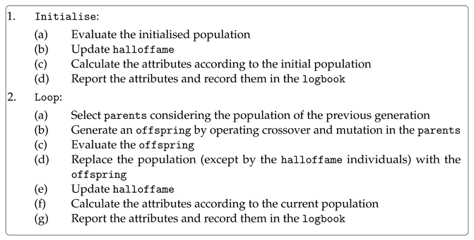
The algorithm ge_eaSimpleWithElitism is summarised in Listing 3. The initialised population is evaluated with the points_train once the first generation starts, and then the halloffame object is updated according to the best individuals found in the population. Next, the attributes to be reported are calculated, and their results are recorded in the logbook. Finally, the initial generation ends, and the algorithm starts a loop to run the remaining generations. The first step is selecting parents according to the method registered in the toolbox. There are selected (population_size – elite_size) individuals as parents each generation. These individuals are operated by crossover and mutation, considering their respective probabilities. Regarding the crossover, all individuals are considered pairwise, and according to the probability each pair is operated on or not, and the point to perform the crossover in each individual is chosen at random within the effective length of the genomes. Before finishing the crossover step, the offspring is mapped in order to get its current effective length before the next operation. Concerning the mutation, all individuals after the crossover procedure (even those which were not operated on) are considered individually. Each codon within the effective length of the genomes is mutated or not, according to the mutation probability. Finally, the offspring is generated, and is evaluated with the points_train. Next, the population is replaced (except by the elite individuals) with the offspring, the halloffame object is updated, the attributes to be reported are calculated, and their results are recorded in the logbook. If the last generation was achieved, the process ends, and the best individual is evaluated with the points_test. Otherwise, the loop continues.

Listing 3. Basic algorithm for GE on GRAPE.

Once the evolution is completed, we can take results from some objects. In the population we have the attributes (genome, phenotype, depth etc.) of all individuals in the last generations, while in the halloffame we have the attributes of the elite_size best individuals. However, the main source of results is found in the logbook, where the statistics over all the generations are registered. These results can be used to build graphs showing the performance in one run, or we can easily perform multi-runs, each time stacking the final logbook in a list, which will be used to build graphs showing the average performance in multi-runs. Another option is to save the results of each runs in an external file such as a .csv for posterior use.

4. General Experiments

We perform three different comparisons in this section. In the most important one, we compare the results of GRAPE against PonyGE2 in four datasets, showing results related to the performance and carrying out statistical analyses to substantiate our observations. We aim to show that there are no significant differences between the results, and therefore that it is worthwhile to use GRAPE due to the advantages such as the easy manipulation of the evolutionary mechanism and the compatibility with other tools already that it inherits from DEAP. In this comparison, we run experiments with two well-known regression problems (Pagie-1 and Vladislavleva-4) and two binary classification problems (Banknote and Heart Disease). Secondly, we run other experiments using only GRAPE to exemplify the use of its different tools. We use different initialisation methods with the same datasets previously mentioned, and we also compare lexicase selection with tournament selection when evolving two distinct Boolean problems (11-bit multiplexer and 4-bit parity) traditionally used as benchmarks in evolutionary algorithms.

Vladislavleva-4 is a benchmark dataset for regression, produced with the following expression, in which the training set is built using 1024 uniform random samples between 0.05 and 6.05, and the test set with 5000 uniform random samples between −0.25 and 6.35.

$$y=\frac{10}{5+{\sum }_{i=1}^5{(x_i-3)}^2}$$

(1)

Another benchmark dataset for regression used in this work is Pagie-1. This dataset is produced with the following expression, in which the training set is built using a grid of points evenly spaced from −5 to 5 with a step of 0.4, and the test set in the same interval, but using a step of 0.1.

$$y=\frac{1}{1+x_1^{-4}}+\frac{1}{1+x_2^{-4}}$$

(2)

Regarding the classification problems, the Banknote dataset has four continuous features, while the Heart Disease dataset has 76 multi-type features, but only 14 are typically used with Machine Learning experiments [18], this consisting of five numeric and nine categorical features. The dataset has four classes, but in the literature, the last three classes are grouped as one, and the classification indicates the presence or absence of heart disease.

4.1. Experimental Setup

The datasets related to Pagie-1, Vladislavleva-4 and Banknote problems are found in the PonyGE2 GitHub repository [19], and we use their split into training and test sets. We also use their proposed grammars. We split the Heart Disease data into 75% for training and 25% for test, using the same sets in all experiments. Finally, we use the entire dataset as training set when running Boolean problems, since we do not execute a test step.

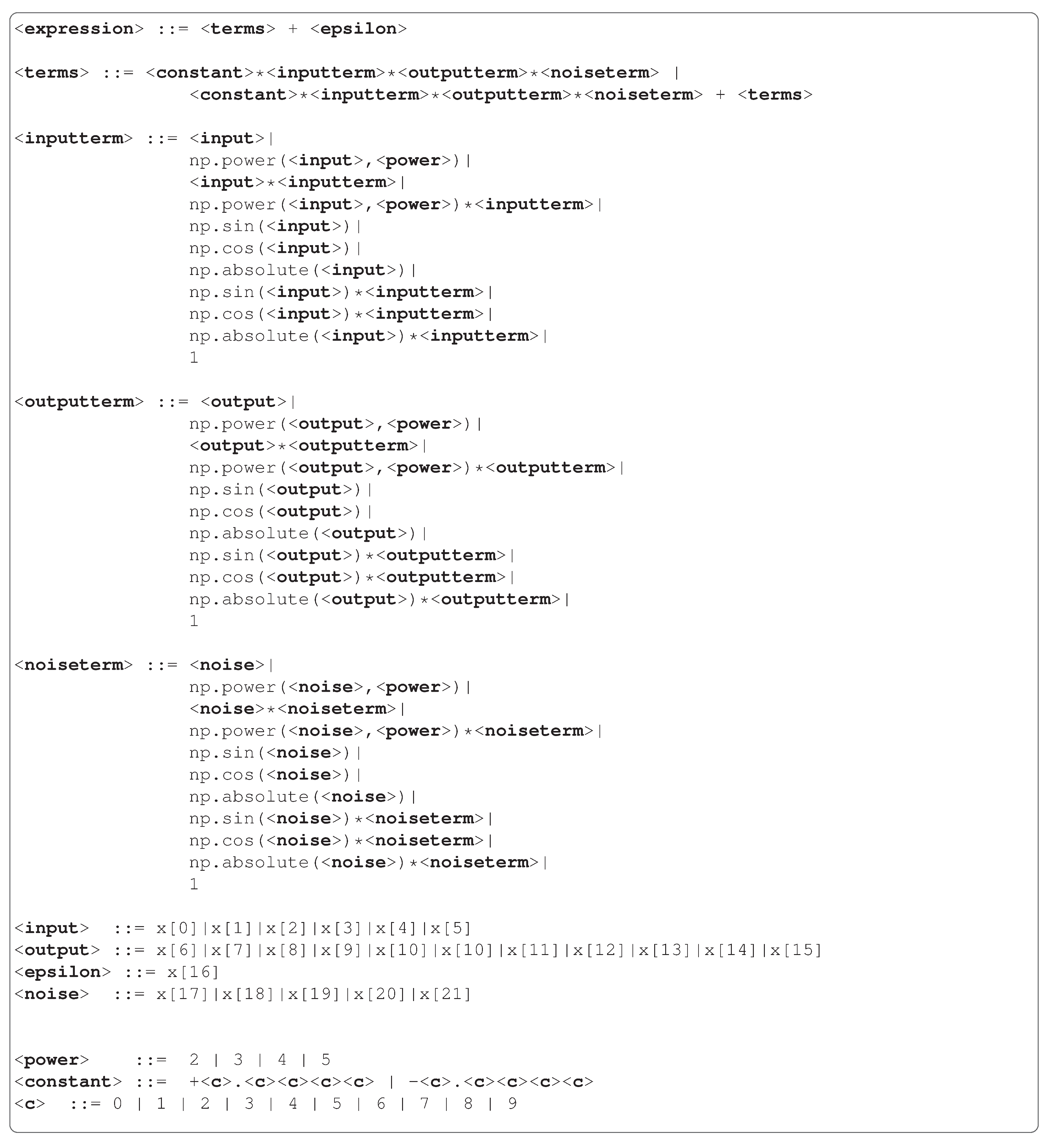
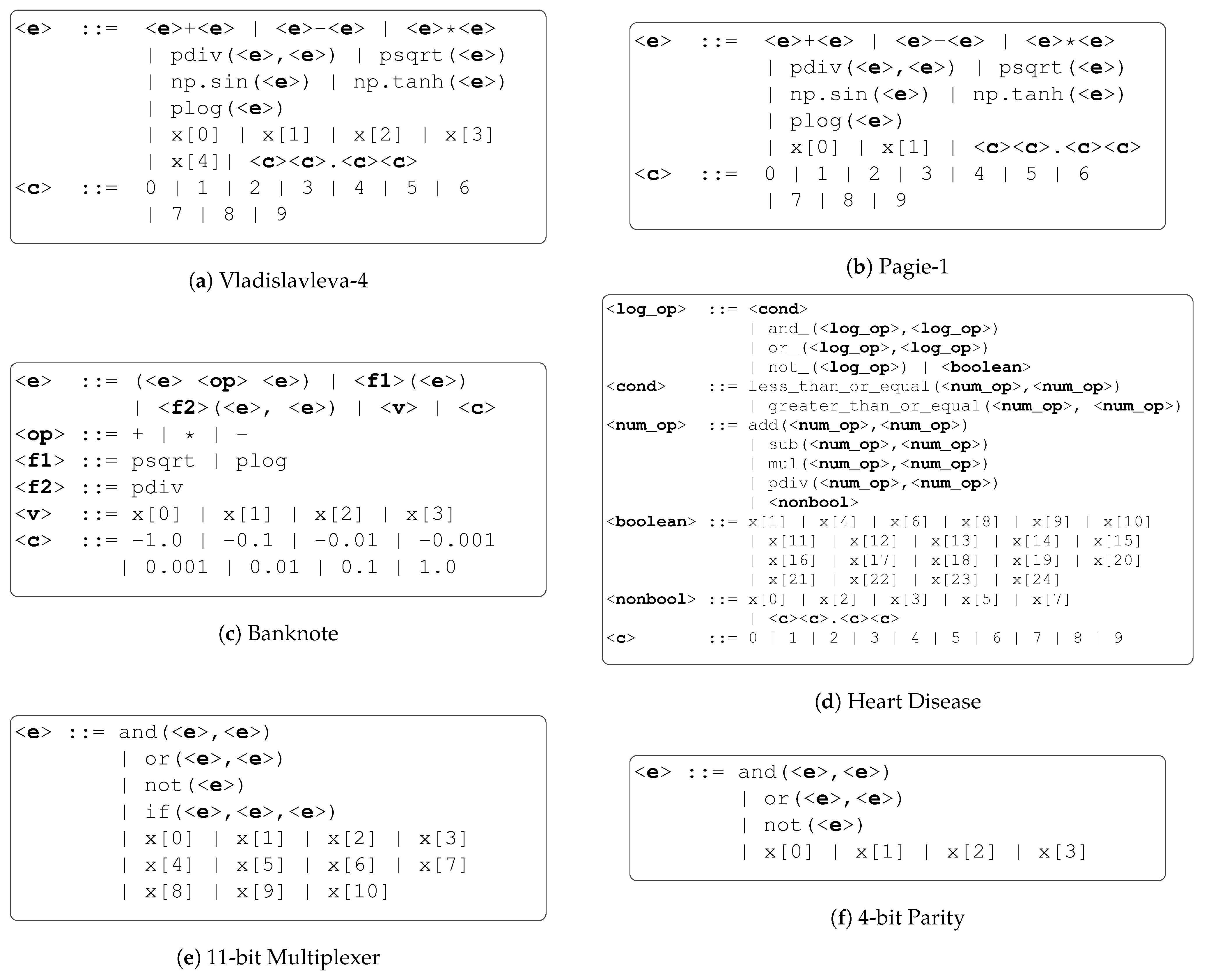
Figure 3 shows the grammars used in our experiments. We execute a preprocessing step for the Heart Disease dataset, in which we normalise the numeric features and use one-hot encoding in the categorical features (except when the feature is already binary). As a result, we have 20 Boolean features and five non-Boolean features, as we can see in the Heart Disease grammar. We have numerical operators to use with non-Boolean features and float numbers, and conditional branches to convert these results into Boolean enabling operations with Boolean features bringing to a binary result. Regarding the Boolean problems, we use the same function sets as Koza [8], which involves the operators AND, OR and NOT, and the IF function, which executes the IF-THEN-ELSE operation.

We summarise in

Table 2. Symbolic regression tableau.

Objective:	Vladislavleva-4: Find a function of five independent variables and one dependent variable that fits 1024 data points, where the target function is seen in Equation (1) Pagie-1: Find a function of two independent variables and one dependent variable that fits 676 data points, where the target function is seen in Equation (2)
Terminal operands:	$X_i$, where i = 1, 2, 3, 4, 5 (Vladislavleva-4) or i = 1, 2 (Pagie-1), and constant values between 0 and 99.99
Terminal operators:	+, −, *, protected div, protected sqrt, sin, tanh and protected log
Fitness cases:	Vladislavleva-4: 1024 uniform random samples between 0.05 and 6.05 Pagie-1: grid of points evenly spaced from −5 to 5 with a step of 0.4
Fitness score:	root mean squared error over all fitness cases

the information related to the regression problems using a style similar to [6,8], and

Table 3. Experimental hyperparameters.

Parameter Type	Parameter Value
Number of runs	30
Number of generations	200
Population size	1000/1000/100/1000/500/500
Elitism ratio	0.01
Mutation probability	0.01
Crossover probability	0.8
Initial genome length	21/24/50/42
Maximum initial depth	10
Minimum initial depth	1/1/1/2/1/1
Maximum depth	90
Codon size	255
Wrapping	0

shows the hyperparameters used in all experiments. We chose these parameters according to the results of some initial runs. In the table, the population size and the minimum initial depth values refer to the Vladislavleva-4, Pagie-1, Banknote, Heart Disease, 11-bit multiplexer and 4-bit parity problems, respectively. We set up the minimum initial depth with the lowest possible value for each problem, considering their respective grammars. The initial genome length parameter is only relevant when running experiments with random initialisation, and in this case the values refer to the Vladislavleva-4, Pagie-1, Banknote and Heart Disease problems, respectively.

When running experiments with random initialisation, we have another parameter, which defines the initial length of the genome. In order to carry out a fair comparison with other methods, we decided to choose this parameter based on the results from sensible initialisation and PI Grow initialisation.

Table 4. Average of the genome length in the first generation in 30 runs using sensible initialisation or PI Grow initialisation on GRAPE.

	Initial Genome Length
	Sensible Initialisation	PI Grow Initialisation
Banknote	44.8	55.8
Heart Disease	38.1	46.2
Pagie-1	21.6	27.1
Vladislavleva-4	16.3	25.6

shows the average in 30 runs of the initial genome length using sensible initialisation or PI Grow initialisation. For the experiments with random initialisation, we used as initial genome length approximately the average of the other methods, which brings the values presented in Table 3.

We use the root mean squared error (RMSE) as fitness metric for the regression problems and the mean absolute error (MAE) for the remaining problems; therefore, we wish to minimise the score. Concerning the lexicase selection process when running Boolean problems, we define the fitness for each sample with two possible values: 1, if the sample was correctly predicted, and 0 otherwise.

4.2. Results and Discussion

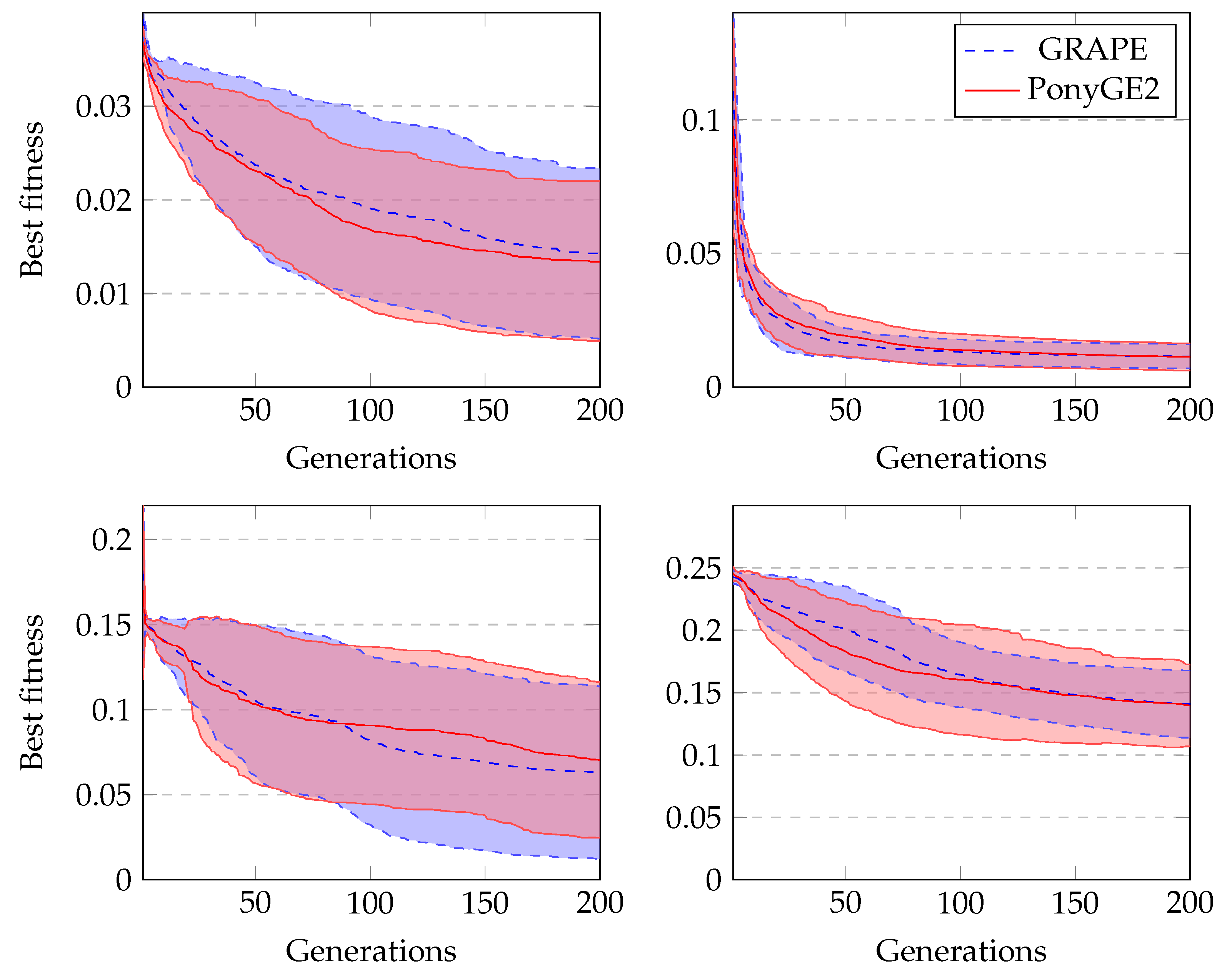
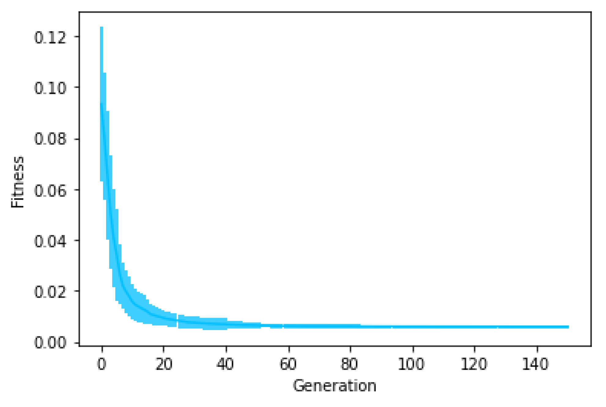
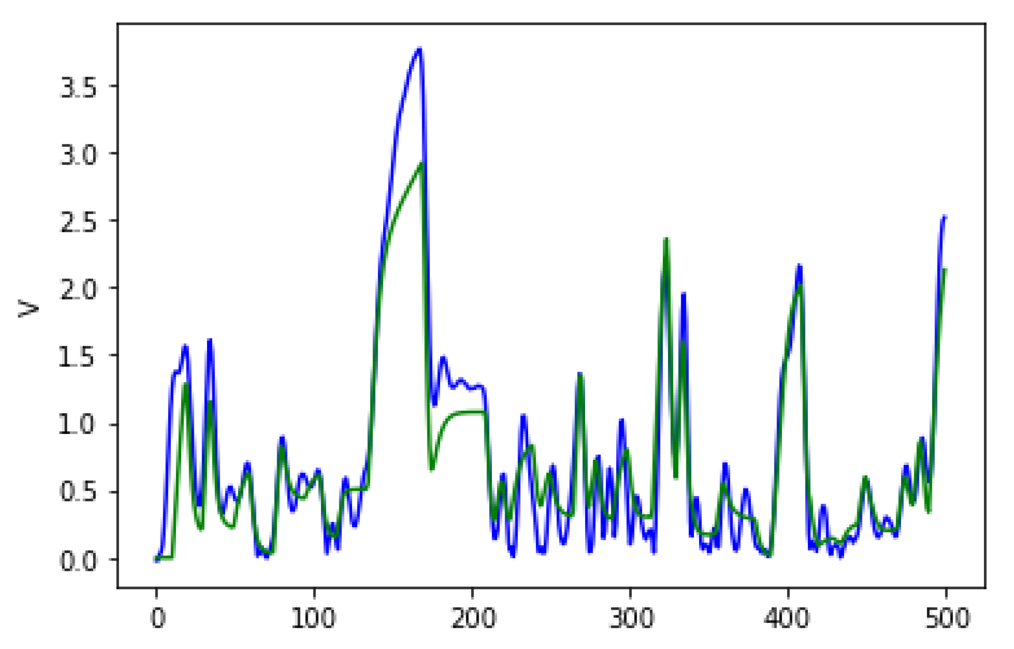
Figure 4 shows the average fitness of the best individual in the training sets across generations using GRAPE and PonyGE2 for each of the experiments. We run all experiments using PI Grow initialisation, tournament selection (size 7), the same parameters and the same grammars. In general, the results are quite similar. In the final generations, the curves are too close for each of the Pagie-1 and Heart Disease problems to distinguish, PonyGE2 is a slightly better with the Vladislavleva-4 problem and GRAPE is a little better on the Banknote problem. We show these results to compare the evolutionary process in both tools, but, of course, test performance is the key goal.

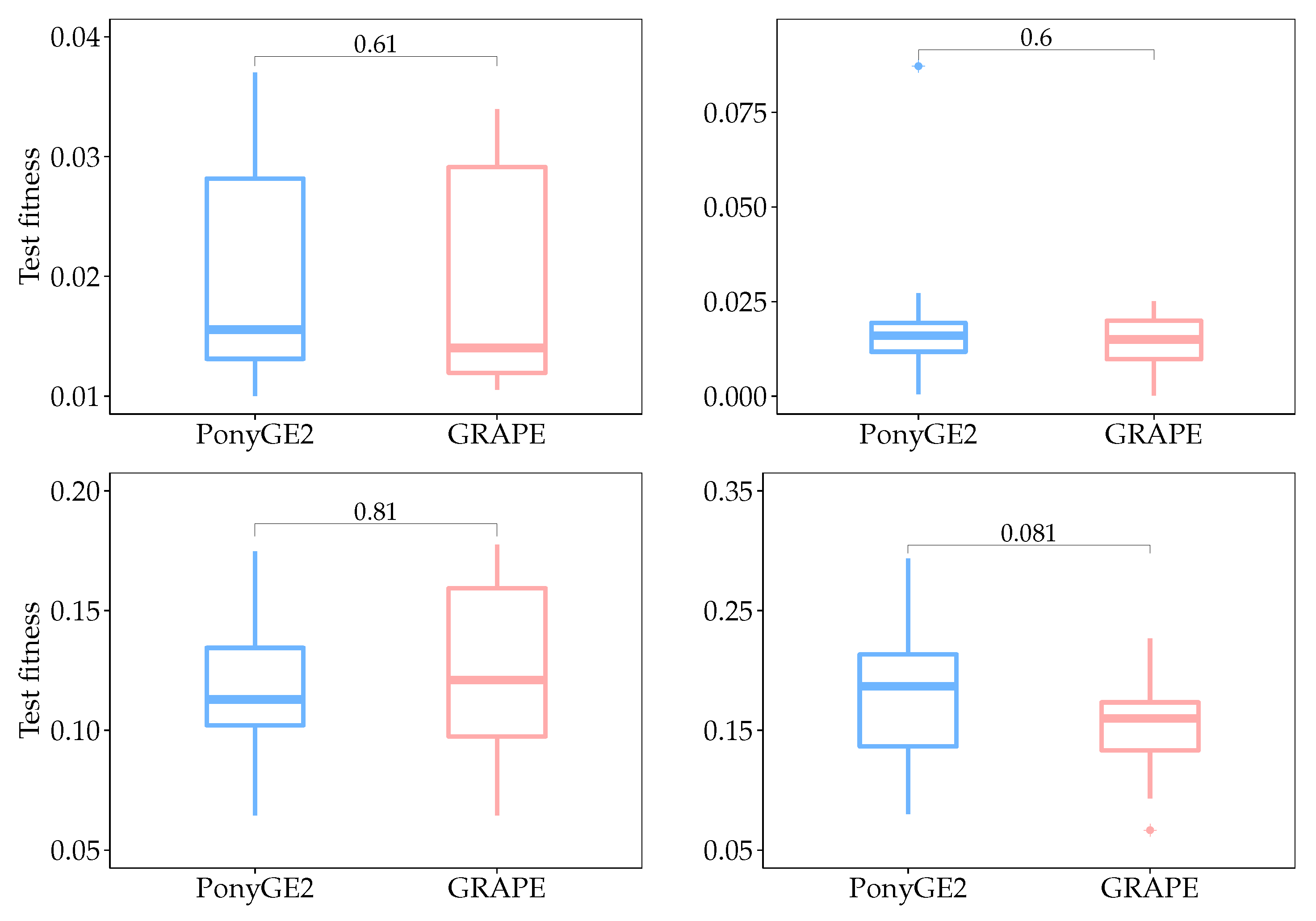
Box plots for test fitness scores for all runs are shown in Figure 5, and their respective p-values calculated using the Mann-Whitney-Wilcoxon test. We used this test since we do not know a priori what sort of distribution the results have, and the aim of this statistical analysis is to check if there is a significant difference between the results using PonyGE2 and GRAPE, which we compared in each problem independently. Given that the null hypothesis says that there is no difference between the results and that we need at most $p=0.05$ to reject it with a confidence level of 95%, we can conclude that there is no significant difference between the results using PonyGE2 and GRAPE on these four problems.

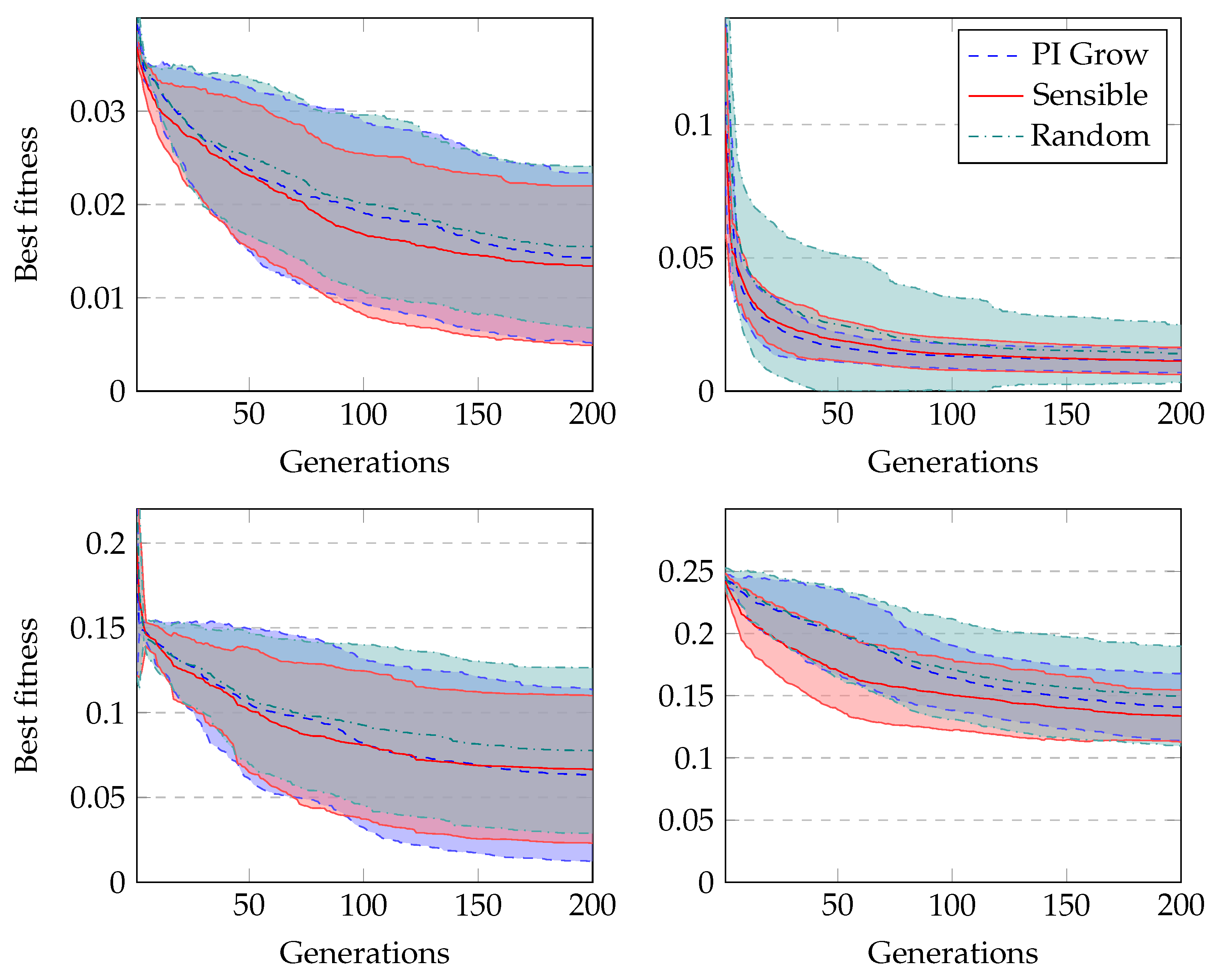
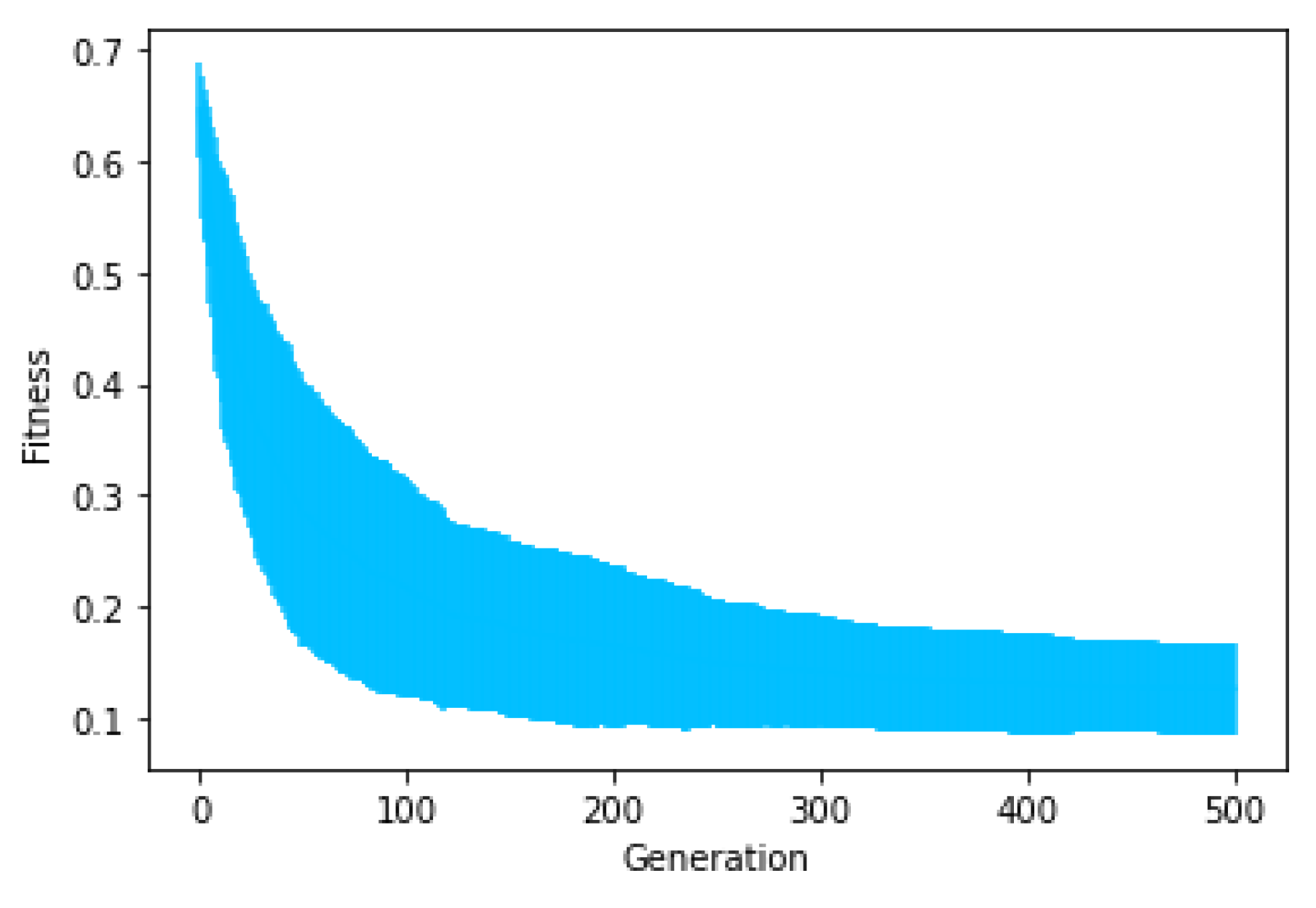
Figure 6 shows the average fitness of the best individual in the training set across generations when using GRAPE with the three initialisation methods. The results are similar in the first generations, but random initialisation presents the worst results for all problems once the evolution advances. This happens because this method cannot create a high-level diversity population. On the other hand, sensible initialisation and PI Grow initialisation present similar results in the final generations for the Pagie-1 and Banknote problems, while sensible initialisation is slightly better for the Vladislavleva-4 and Heart Disease problems.

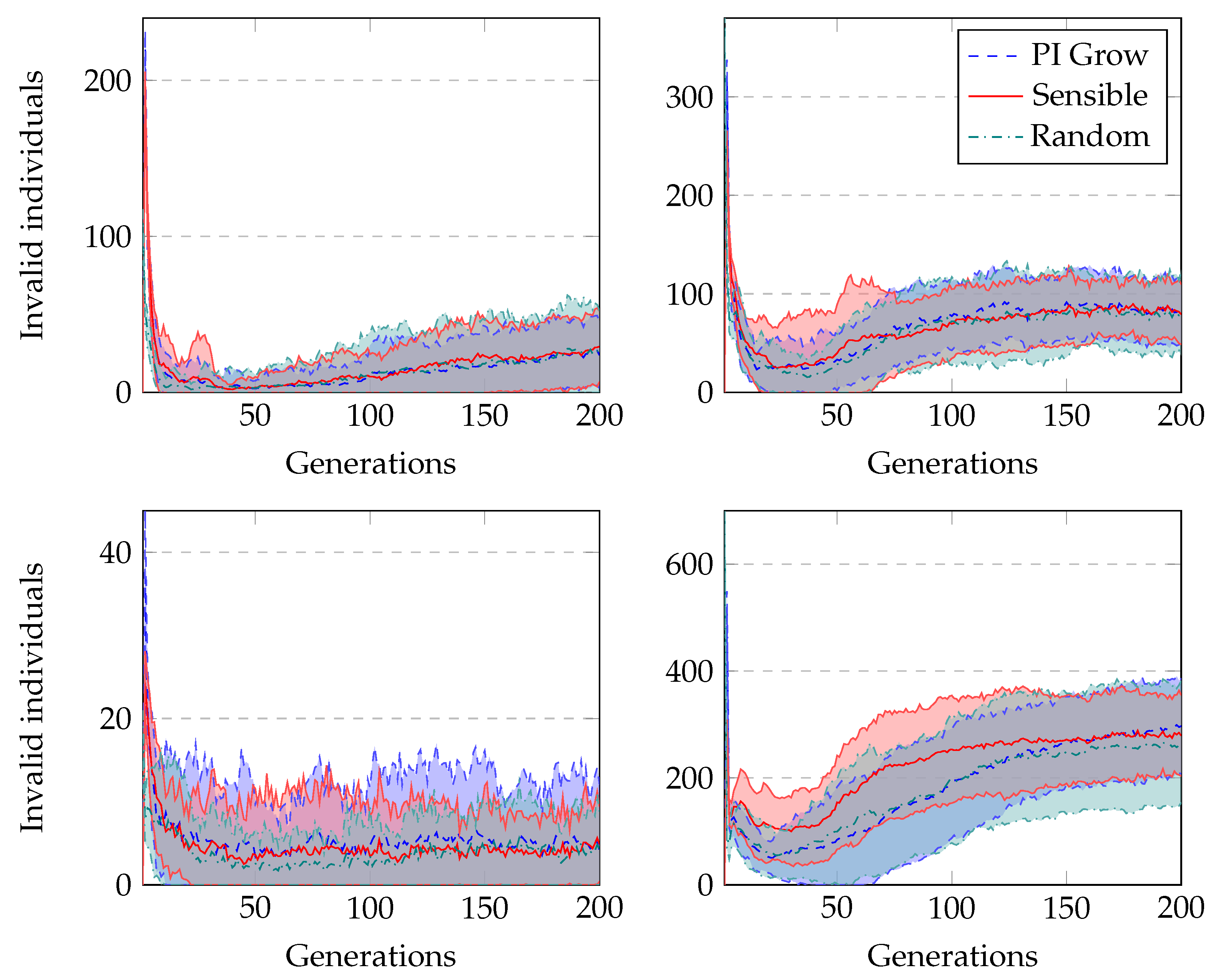
The average number of invalid individuals across generations when running GRAPE with distinct initialisation methods is shown in Figure 7. Both sensible initialisation and PI Grow initialisation start with zero invalid individuals, but in the second generation, both experience the peak of the curves. This is due to the randomness of the tails added to the initial individuals. On the other hand, random initialisation presents its peak of invalid individuals in the first generation. In general, the number of invalids decreases sharply in the first generations as the randomness of the initialisation loses influence on the current population. However, after some generations, this number slightly increases as the individuals in the population increase in size, and therefore become more complex. In this situation, applying crossover or mutation is more likely to invalidate the individuals than in a population with small individuals. Finally, in terms of the percentage of the population representing invalid individuals, the highest value occurs for the Heart Disease problem. This is an expected observation because these experiments use the most complex grammar.

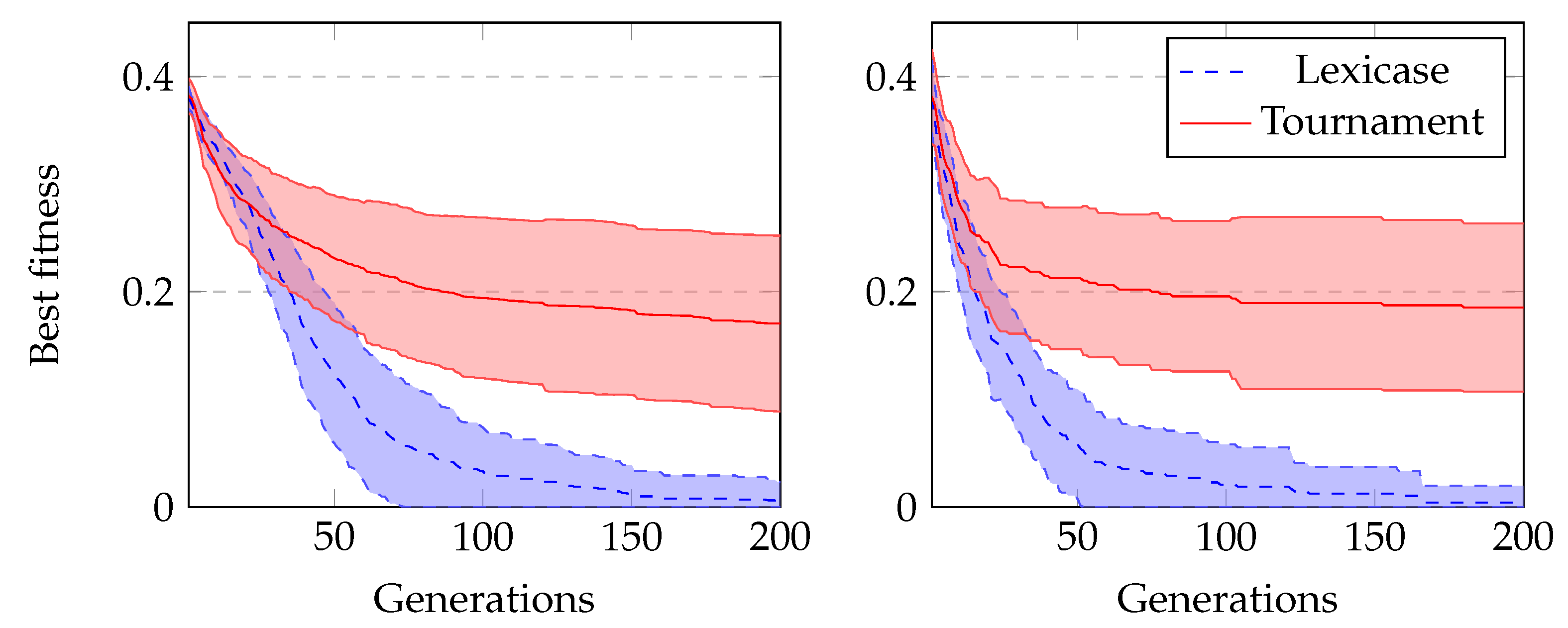
In our final comparison, we run experiments using GRAPE with lexicase selection and tournament selection to evolve Boolean problems. We run all experiments with sensible initialisation. The results using lexicase selection are clearly much better, as we can see in Figure 8. In Boolean problems, since there is no split in training and test sets, we usually also measure the number of successful runs during training. These are runs that achieved a solution that satisfies all cases in the dataset.

Table 5. Number of successful runs in the 11-bit Multiplexer and 4-bit Parity problems.

	Successful Runs (Out of 30)
	11-Bit Multipler	4-Bit Parity
Lexicase selection	27	28
Tournament selection (size 7)	0	1

shows these results, and we can see again a clear superiority of lexicase selection.

5. Signals and Systems Experiments

5.1. Introduction

In this section we use the newly developed GRAPE library on two systems identification benchmark problems: “Silverbox” and “Coupled Drives”. The two data sets are publicly available at the nonlinearbenchmark.org website (accessed on 8 August 2022), a collection of data sets meant to be used in nonlinear system identification tasks [20]. The use of Evolutionary Computation methods for identifying dynamical systems is a common approach, since this task can be interpreted as an special case of symbolic regression, and most of these algorithms are capable of finding model structures and estimate parameters in optimal or close-to-optimal fashion. When a fixed structure is known a priori, for example, a simple GA can be used for parameters estimation, while GP or GE can search for both a structure and parameters at the same time during evolution. When presenting GP in his seminal work, John Koza has suggested system identification as one class of problems that could be solved by his technique [8], a suggestion since validated by the substantial literature on the field [21]. Grammar-based techniques have also been applied to these problems, bringing some advantages such as the possibility of limiting the search scope into a specific class of models (e.g., ARX, ARMAX, NARMAX, etc.) [22] and incorporating problem-specific knowledge, such as signal periodicity [23].

Another specific aspect of system identification problems is the differentiation between prediction error and simulation error. In one-step-ahead prediction the model has access to both previous input and output data from the original data set, while in simulation the model is presented only with input data, and any autoregressive term must use previous outputs from the simulation itself, not from the data set. This difference when sourcing data can result in completely different behaviours for a given model when submitted to prediction or simulation: very often models that present a low prediction error end up being unstable or presenting a much higher error rate when submitted to free-run simulation. The main reason for this is the fact that small output errors in simulation get fed back into the system, getting accumulated and amplified, while in prediction the model can always go back to the “ground truth” of the original data set, preventing its output from drifting too much [24]. This difference in performance between prediction and simulation errors can be seen on the experiments performed in this work, where despite the good simulation results that have been achieved, prediction errors are always significantly lower. Also, obtaining the simulation error is typically more computationally expensive than obtaining the prediction error. A compromise between both can be achieved with k-step-ahead prediction, where simulation can run freely for a specified number of steps (k) before using the original data again.

Therefore, results for system identification experiments are typically reported using their simulation errors, which is a challenge itself in some cases, given the extra computational effort required for simulation in comparison with prediction. In this work we use the prediction error as the main driver for the evolution process, since we use the prediction root mean squared error (RMSE) as the fitness function used for selection, but all results are reported on the best obtained simulation error. While there is no guaranteed correlation between prediction error and simulation error for a given individual, a population-based approach such as GE can benefit from the use of the less expensive prediction error in the evolutionary loop while only the best performing individuals are simulated. The rationale is that within a large enough population of solutions at least one good performing individual in terms of prediction will also eventually present a low simulation error. Another approach often used in EC experiments is the parameters tuning of the best or all individuals after each generation, which would adjust constants associated to a given model structure in an effort to reduce its error or even bring it back from instability. For linear-in-the-parameters models, well known techniques such as the least squares approach can be applied to this optimisation step. We envisage that, as future work, such techniques will be integrated into GRAPE.

5.2. The Silverbox Data Set

The “Silverbox” data set is one of the three nonlinear system identification benchmark problems published by Wigren and Schoukens in a paper from 2013 [25]. The paper introduces data sets “collected from laboratory processes”, i.e., empirical data, instead of simulations. It uses an electrical circuit to represent a nonlinear mechanical resonating system constituted of three elements: a moving mass, m, a viscous damping, d, and a nonlinear spring that depends on displacement, k(y). The circuit is then responsible for relating the output y(t) (displacement), with the input force u(t). The system can be represented by the following differential equation:

$$m\frac{{\mathrm{d}}^{2}y\left(t\right)}{\mathrm{d}{t}^2}+d\frac{\mathrm{d}y\left(t\right)}{\mathrm{d}t}+k\left(y\left(t\right)\right)y\left(t\right)=u\left(t\right),$$

(3)

while the position-dependent nonlinear spring stiffness can be described by the following quadratic equation:

$$k\left(y\left(t\right)\right)=a+b{y}^2\left(t\right).$$

(4)

The resulting data set has a high enough signal to noise ratio so measurement noise can be discarded, and it is generated in two parts: on the first one, with 40,000 samples, the reference signal r(k) is given by a Gaussian white noise sequence filtered by a 9th order discrete Butterworth filter (cut-off frequency of 200 Hz), and the amplitude was linearly increased from zero to approximately 150 mV maximum. On the second part the reference signal consisted of a sequence of 10 successive realizations of a random odd multi-sine signal of frequencies also up to 200 Hz, given by

$$r\left(k\right)=A\sum _{l=1}^{l_{max}}cos(2\pi f_{0}l+{\phi }_l).$$

(5)

where A is the amplitude, in V, k is the index of the sample, l is the index of the different sine waves, $f_0$ is the base frequency (derived from the sampling frequency, as explained in [25]) and ${\phi }_l$ is a uniformly distributed phase value.

The ten consecutive realizations of the multi-sine signal were concatenated with sequences of 100 zeros to indicate the end and start of each new realization. The sampling frequency for the data acquisition was set to 610.35 Hz, and further information regarding the equipment used in the signal generation and data acquisition, as well as the experiment setup can be retrieved from the original paper [25]. For the evolutionary experiments conducted in this paper we have followed the data split proposed by Kandhelwal et al. [22]: the first nine out of the ten sinusoidal realizations have been used for training (parameters and structure estimation), with the remaining one being used as the validation set. The resulting models were then evaluated regarding their prediction and simulation errors on the first 40,000 samples.

5.3. The Coupled Drives Data Set

The data set called “Coupled Drives” is also described by Wigren and Schoukens [25], and is another example of empirical data generated from a laboratory process. The physical process consists of two electrical motors connected to a pulley trough a flexible belt, while the pulley itself is held by a spring, resulting in a slightly damped dynamic. Both electric motors can be controlled individually, what also allows for the speed and tension on the belt to be controlled simultaneously. Movement is possible in both clockwise and counterclockwise directions, and a pulse encoder is used for measuring the speed, which is insensitive to direction, i.e., velocity in both directions is always registered as a positive value. Furthermore, there are low-pass and anti-aliasing filters at the output signal. A possible representation of the system on discrete time presented by the authors is given by the following equations, where the input $u\left(t\right)$ is considered to be the sum of the voltages applied to the motors and $y_n\left(t\right)$ the output signal:

$$y\left(t\right)=\frac{b_1{q}^{-1}+b_2{q}^{-2}+b_3{q}^{-3}}{1+f_1{q}^{-1}+f_2{q}^{-2}+f_3{q}^{-3}}u\left(t\right)+w\left(t\right),$$

(6)

$$y_n\left(t\right)=\left|y\left(t\right)\right|+e\left(t\right),$$

(7)

where b and f are the model parameters and $e\left(t\right)$ and $w\left(t\right)$ are disturbances. The Authors also present a Wiener-Hammerstein model for the same process, not demonstrated here. The resulting data set from the “Coupled Drives” experiment was generated using two types of inputs on the electric motors: first a Pseudo-Random Binary Signal (PRBS) ranging from a negative to a positive value $\pm u_{PRBS}$ in three different open loop realizations ($u_{PRBS}$ = 0.5, 1.0 and 1.5 V). The second input signal was generated from a PRBS with a clock period of five times the sampling period, this time switching between −1.0 V and 1.5 V on a first realization and −1.0 V to 3.0 V in a second realization. The signal was then multiplied by a random number coming from a uniform distribution ranging from 0 to 1. Both types of inputs were sampled using a 20 ms period, and because they switch between positive and negative numbers, the direction of the belt rotation was also frequently changing. The different realizations resulted in data sets containing 500 samples each, and in this work we follow the same data split used by Nechita et al. [26]: the first realization of the uniformly distributed inputs is used as training data, while the second one is used for test and results reporting.

5.4. Experimental Setup

The system identification of the described data sets was performed using the GRAPE library in several evolutionary experiments, each one consisting of 50 different runs, with the best model emerging from these runs used for reporting prediction and simulation errors. A parallelisation strategy based on the “multiprocessing” Python library was implemented to speed up the process, allowing it to perform several simultaneous concurrent evolutionary loops. For the Silverbox problem a grammar capable of generating NARMAX models was used, while the Coupled Drives problems used the same grammar extended with the cos, sin and absolute functions, given the characteristics of the physical process [26]. An autocorrelation analysis was also performed in both data sets in order to define the scope of past observations of inputs, outputs and noise terms that would be available in the grammar, instead of using a lag operator. Therefore, a lag matrix was generated from the original data set and the grammar, as implemented in [23], was seeded with the highest autocorrelated terms: inputs up to $u(k-5)$, outputs up to $y(k-10)$ and noise terms up to $w(k-5)$. The extended grammar can be seen in Listing 4, while the evolution hyperparameters used in both case studies are presented in

Table 6. Experimental hyperparameters for the two system identification case studies.

Parameter Type	Parameter Value
Number of runs	50
Number of generations	500
Population size	100
Elitism ratio	0.01
Mutation probability	0.01
Crossover probability	0.99
Maximum initial depth	20
Minimum initial depth	5
Maximum depth	150
Codon size	255
Wrapping	0

:

Listing 4. Extended NARMAX grammar used in the Coupled Drives problem. A similar one, without the sin, cos and absolute functions was used for the Silverbox problem.

5.5. Results

This subsection presents the results obtained on the identification of the two systems.

Table 7. Experimental results from the Silverbox problem.

Metric	Value
Simulation RMSE	0.01295
Prediction RMSE	0.00529
Average Min RMSE (Prediction)	0.00587
Standard Deviation	0.00059
Elapsed time (50 runs)	27,550.79 s
Average time per run	551.02 s

contains the numerical results for the Silverbox problem, while Figure 9, Figure 10 and Figure 11 depict, respectively: the average minimum prediction RMSE for the validation data over the 50 runs, the predicted output from the best individual (green) compared to the empirical data (blue), and the simulated output from the best individual (green) also compared to the empirical data (blue).

Table 8. Experimental results from the Coupled Drives problem.

Metric	Value
Simulation RMSE	0.28148
Prediction RMSE	0.08008
Average Min RMSE (Prediction)	0.12584
Standard Deviation	0.04074
Elapsed time (50 runs)	1413.20 s
Average time per run	28.26 s

and Figure 12, Figure 13 and Figure 14 present the same information, but for the Coupled Drives problem.

5.6. Discussion

As shown in Section 5.5, GRAPE has been successfully used for two benchmark nonlinear system identification problems. The “fitness over generations” graphs presented a typical convergence behaviour expected in evolutionary experiments, while the prediction and simulation output graphs show results that are stable and close to the target empirical data also in the time domain. As expected and discussed in Section 5.1, the simulation results were in both cases slightly worse than prediction results for both problems. This difference can be clearly seen when comparing Figure 13 and Figure 14 for example, where the best individual on simulation captures the overall behaviour of the system, but struggles to match perfectly all the oscillations seen on the empirical data like prediction does.

While these results outperform some works currently reported in literature [27,28], we are aware of other authors that were capable of achieving better results than ours using other approaches [20]. However, we highlight that the intent of these case studies was mainly to illustrate the use of GRAPE and Grammatical Evolution in system identification problems approached from a symbolic regression perspective, and no extra optimisation steps currently seen in literature such as parameters tuning, local search or multiobjective approaches have been implemented. Nevertheless, we believe that GRAPE offers a user-friendly and robust platform for system identification problems that can yield competitive results, specially considering the potential for the implementation of these and other further optimisation techniques in future works.

6. Conclusions

We have described a new implementation of GE in DEAP, a powerful EA framework in Python. We presented a short overview introducing the main topics of GE to new users as well as the algorithm already implemented on GRAPE. We showed some examples of its general use, with different initialisation methods and selection methods. We also performed a comparison with PonyGE2, an existing Python implementation of GE, in which GRAPE was able to achieve similar performance.

Using DEAP brings many advantages, as it is comes with many built-in features that GRAPE inherits, including selection schemes and even search techniques. Future work will consider the impact of different search techniques on these and more problems, to assess if evolution is the most appropriate search engine to use.

The source code of GRAPE, as well as some examples, is already available on the BDS GitHub repository (https://github.com/UL-BDS/grape accessed on 8 August 2020). We plan to make extensive documentation available there for GRAPE as well as any other algorithm, initialisation method, selection method etc., which we implement for our own research work in the future. As a short-term plan, we intend to develop some examples using the multi-objective optimisation tools already implemented on DEAP.