Article

On the Quality of Deep Representations for Kepler Light Curves Using Variational Auto-Encoders

1
Department of Informatics, Federico Santa María Technical University, Santiago 8940572, Chile
2
Department of Electronics, Federico Santa María Technical University, Valparaíso 2390123, Chile
*
Author to whom correspondence should be addressed.
Signals 2021, 2(4), 706-728; https://doi.org/10.3390/signals2040042
Submission received: 1 April 2021 / Revised: 16 August 2021 / Accepted: 8 October 2021 / Published: 14 October 2021
(This article belongs to the Special Issue Machine Learning and Signal Processing)

Abstract

:
Light curve analysis usually involves extracting manually designed features associated with physical parameters and visual inspection. The large amount of data collected nowadays in astronomy by different surveys represents a major challenge of characterizing these signals. Therefore, finding good informative representation for them is a key non-trivial task. Some studies have tried unsupervised machine learning approaches to generate this representation without much effectiveness. In this article, we show that variational auto-encoders can learn these representations by taking the difference between successive timestamps as an additional input. We present two versions of such auto-encoders: Variational Recurrent Auto-Encoder plus time (VRAE t ) and re-Scaling Variational Recurrent Auto Encoder plus time (S-VRAE t ). The objective is to achieve the most likely low-dimensional representation of the time series that matched latent variables and, in order to reconstruct it, should compactly contain the pattern information. In addition, the S-VRAE t embeds the re-scaling preprocessing of the time series into the model in order to use the Flux standard deviation in the learning of the light curves structure. To assess our approach, we used the largest transit light curve dataset obtained during the 4 years of the Kepler mission and compared to similar techniques in signal processing and light curves. The results show that the proposed methods obtain improvements in terms of the quality of the deep representation of phase-folded transit light curves with respect to their deterministic counterparts. Specifically, they present a good balance between the reconstruction task and the smoothness of the curve, validated with the root mean squared error, mean absolute error, and auto-correlation metrics. Furthermore, there was a good disentanglement in the representation, as validated by the Pearson correlation and mutual information metrics. Finally, a useful representation to distinguish categories was validated with the F 1 score in the task of classifying exoplanets. Moreover, the S-VRAE t model increases all the advantages of VRAE t , achieving a classification performance quite close to its maximum model capacity and generating light curves that are visually comparable to a Mandel–Agol fit. Thus, the proposed methods present a new way of analyzing and characterizing light curves.

1. Introduction

New instrumentation technologies, such as the Legacy Survey of Space and Time (LSST) at the Vera C. Rubin Observatory [1], the Transiting Exoplanet Survey Satellite (TESS, [2]), and future space-based telescopes and ground-based observatories have motivated the use of automatic techniques to process and analyze the large amount of data that is being and will be generated.
In the exoplanet domain, advances in instrumentation and data analysis have allowed the discovery of thousands of exoplanets. NASA has reported (last updated 12 October 2021: https://exoplanets.nasa.gov accessed on 13 October 2021) more than 4500 exoplanets detected using different techniques, despite the fact that planets emit or reflect very faint light compared to their host star and that their orbital distance is very small relative to observational distance. The analysis of light curves has been the main source of candidate objects. These series are photometric observations of light intensity as a function of time, where the observed star luminosity varies through time as a result of intrinsic processes or due to external influences, such as an orbiting planet passing between the star and the observer. The latter phenomenon is called a transit and has been used as an effective method (http://exoplanetarchive.ipac.caltech.edu/docs/counts_detail.html accessed on 12 October 2021) method to study candidate orbiting objects. A transit light curve can be mathematically modeled as a natural phenomenon of an orbiting object, and algorithms such as the well-known Mandel–Agol method [3] can be used to fit such models. Unfortunately, the diversity of planetary systems (and their corresponding astrophysical scenarios) prevents unique model selection due to the unknown number of transits and complex dynamics, such as eclipsing binary systems, very faint observation, or the microvariability of the star [4].
The application of task-based learning models to solve specific tasks (e.g., exoplanet search) has been the common approach to reduce human effort [5,6,7,8]. These are methods that learn representations and model parameters based on a specific learning task and a particular objective function, usually based on the available labels. On the other hand, learning models to build self-generated representations of light curves have been largely unexplored.
Task-free methods, such as those in [9,10,11], learn the key features (representation) for detecting candidate exoplanets from data instead of imposing a model without the correct capacity to learn the task (i.e., excessively simple or complex for the observed data). These methods learn pattern structures from the data without the need for labels (i.e., unsupervised learning), having the advantage of using all the available data.
A major challenge of working with time series in astronomy is that they are usually noisy, meaning that values are missing for several timestamps or that the measurements are not uniform throughout the series. Different approaches have been proposed to solve this representation issue such as binning the light curve based on a previous folding of the periodic behavior [6], extracting specialized features based on subsets of data points [12], or explicitly modeling the time dependencies [13]. Based on the latter, some approaches have included the time information in the input representation of the learning model, showing improved results [10,14,15].
Motivated by the success of deep learning techniques [16] in different research fields, we focused on using the auto-encoder models. In this paper, we propose using variational (stochastic) models as dimensionality reduction techniques in order to learn a quality deep representation for Kepler light curves. Specifically, we propose two variational recurrent auto-encoder extensions that can process the noisy Kepler time series by using the time information of each observation. We extend the idea of using all the information on the time series by including the standard re-scaling pre-processing task into the learning model as an end-to-end architecture. The motivation to extract the information on the original scale of the light curve, based on Flux standard deviation (F-std), emerges from the fact that the relative sizes of exoplanets and noise are correlated with the F-std of the signal.
The concept of quality used and proposed in this paper is based on obtaining a compact yet robust representation (i.e., parsimonious), with the capability of smooth time series and with less correlated features (disentangled). In addition, good quality should imply an informative representation of the behavior on the time series, for example by having a better performance on classification tasks (such as time series categories). The need to learn quality representation in astronomy has potential uses in cases such as denoising, large-scale data processing, clustering, manifold learning, characterization, and other unsupervised applications.
Our experiments show that the proposed variational models are robust in learning patterns with less noise (denoising effect), having a balanced behavior between reproducing the original time series and smoothing. Indeed, the resulting light curve could be compared to the isolated simulation of a transit object. The proposed quality factor of the representation was also achieved, representing an improvement over the deterministic counterparts proposed thus far.
This paper is organized as follows. In Section 2, the main methods for light curve representation are jointly described with our proposed methods and their main differences. Then, the experiment setting and results were introduced in Section 3. A brief discussion is presented with regard to the advantage of the proposed methods in Section 4. Finally, Section 5 summarizes the conclusions of this work.

2. Materials and Methods

We review the most relevant current works for light curve representation in Section 2.1. Then, we introduce the proposed methods for learning light curve representation in Section 2.2, a simple extension in Section 2.2.2, and another more complex in Section 2.2.3.

2.1. Light Curve Representation Methods

A light curve is a time series (function of time) containing measurements of the light intensity of a celestial object or region. When one celestial body crosses in front of another astronomical object and blocks any fraction of its light, it is called a transit. In this section, we briefly introduce different representation approaches used to study transit light curves (detection, vetting, classification, characterization) and related fields with model-based and self-generated representations.

2.1.1. Model-Based Representations

The Mandel–Agol simulation [3] models the transit of a spherical planet around a spherical star assuming a non-linear limb darkening model on the light source. It does this by modeling the opacity observed on the light intensity according to the planet’s position with a function over time c ( t ) . When the planet is in front of the star, the opacity is at maximum ( c < 1 ). On the other hand, when the planet orbits without blocking the star light, the opacity is minimum ( c = 1 ). When the planet is close to being in front of the star, the intensity c ( t ) is modeled as a polynomial based on the limb darkening of the star. This requires knowing the distance from the center of the planet to the center of the parent star, as well as the radius of each one of the bodies, the transit period, the inclination, and the limb darkening models (coefficients). There are techniques that find the model parameters through least squares (LS) or Markov Chain Monte Carlo (MCMC).
However, light curves can be observed not only by a transit, but several inherent and exogenous processes might be involved in the variability of the observed intensity of a star. Therefore, several machine learning techniques have been used to classify variable stars, typically by manually extracting specialized features from the light curve as representation and then applying classic pattern recognition methods to them. For example, Richards et al. [12] presents a catalog of variable stars where 53 specialized features are extracted from light curves through statistics such as kurtosis, skewness, standard deviation, and Stetson, plus other features based on the period and frequency analysis of a Lomb–Scargle [13] fitted model. Donalek et al. [17] also worked on classifying variable stars on the Catalina Real-Time Transient Survey (CRTS) and the Kepler Mission, extracting similar features from the light curves. In the work of Nun et al. [18], statistical descriptors are used as inputs for a random forest algorithm that can detect anomalous light curves based on probabilistic learning models. These outliers are removed from the training set used in variable stars’ classification.
For transit vetting, we found the so-called Autovetter [5] which uses the random forest model over the features derived from the statistics pipeline on the Kepler mission for vetting candidate objects on the Kepler Threshold-Crossing Event (TCE) data. Another approach is to represent the light curve as phase-aligned sections called “folds” to address the problem of irregular sampling in transits. This folded light curve centers the transit and stacks all the times on which it occurs, as shown in Figure 1. In this sense, the most common is to bin the folded light curve based on a window proportional to the estimated transit period. For example, as a dimensionality reduction method (embedding representations) of folded light curves, Thompson et al. [11] proposed a locality preserving projection to filter out light curves with non-transit-like shapes, while Armstrong et al. [19] proposes a self-organization map on the classification of true planets.
Neural networks and deep learning [16] algorithms have become very popular in solving problems where feature extraction from data is non-trivial. These algorithms have been successfully applied for transit vetting in recent years by using the binned folded light curve representation. For example, Shallue & Vanderburg [6] used a one-dimensional convolutional neural network (1D CNN) model on vetting candidate exoplanets on the Kepler TCE data with the global and local representation of the folded light curve. Pearson et al. [7] used a similar approach to [6] for detecting transit shape objects trained on simulated data and evaluated using the Kepler mission dataset. Schanche et al. [8] also used a 1D CNN model for distinguishing and vetting candidate exoplanets among variable stars (four classes) on the Wide Angle Search for Planets dataset.

2.1.2. Self-Generated Representations

While most of the representations focus on using astrophysical knowledge to ease a specific task (task-based), e.g., classifying star variability or vetting transits, only a few of them tried different representation approaches without direct human intervention or being especially designed for some task (task-free), which may have the advantage of using unlabeled data and being used for different purposes. Mackenzie et al. [9] used an unsupervised learning algorithm known as affinity propagation with a custom distance function to build a new representation from light curves and then use it on a linear support vector machine to classify variable stars. The representation is based on the similarity between fragments of the light curves and cluster exemplars or centroids. Bugueño et al. [20] also used an unsupervised learning algorithm to build a new representation on the Kepler mission, and in a second phase, used supervised learning to classify true planets. The principal component analysis (PCA) to extract features on the frequency domain representation of light curves, based on a discrete Fourier transform, was used in [20].
In the work of Mahabal et al. [21], an image representation (i.e., grid) was obtained from the variations of magnitude through time from light curves with missing values. This work used the variable star data from the CRTS dataset and completed the classification task using two-dimensional convolutional neural networks (2D CNN), which are models that learn local spatial dependencies [22]. Aguirre et al. [14] also obtained variations in magnitude from variable stars light curves and the delta times of each sample. These were used as different input channels to train a 1D CNN classifier with shared-weights through novel data augmentation techniques.
In the work of Naul et al. [10], time was used as an additional input channel but through recurrent neural network (RNN) models, which are models that learn temporal dependencies [23]. Naul et al. [10] presented a recurrent auto-encoder (RAE) that learned how to embed and then reconstruct a light curve by setting the original times using RNN models in the encoder and decoder phase—which we named “RAE t ” (RAE plus time information). The authors in [10,15] showed that learned representations are useful for classifying variable stars, thus improving the results obtained using statistical features [12]. It also explores the use of the folded light curve representation which further improves the obtained results.
Other types of research have been performed to characterize noisy signals. The most common approach is to estimate the missing values. Rehfeld et al. [24] presented the principal techniques used to analyze the correlation on irregularly sampled time series. Mondal & Percival [25] proposed an estimator for wavelet variance for time series with missing data. There is also the Lomb–Scargle periodogram [13] for period analysis on data with missing values and the previously discussed Mandel–Agol model.
Marquardt & Acuff [26] included delta times (time differences between two adjacent samples) to obtain a spectral analysis from time series. However, to the best of our knowledge, including delta times as an input in neural networks models of noisy times series was first explored by Che et al. [27]. This study presents a modification of a gated recurrent unit (GRU) model [28], namely GRU-D, which uses a binary mask for missing values and the delta times as input channels. The objective was to impute (fill) the missing values to improve the predictions on medical problems.

2.1.3. Variational Auto-Encoders

The variational auto-encoder (VAE) is a stochastic auto-encoder (AE) learned in a probabilistic fashion based on the variational lower bound or evidence lower bound. The VAE framework [29] is extended to work with uniform time series on the variational recurrent auto-encoder (VRAE) proposed by Fabius & van Amersfoort [30]. The motivation behind this is that VAEs are deep generative models trained on an unsupervised scenario, learning latent variable representation as it trains. These variables are learned through the observed distribution, so they are built to adapt to the variations in the behavior of the data. This is the main difference of standard (deterministic) AEs that learn an invariable specific point for the input pattern [31].
The use of the VRAE on different time series applications is associated with anomaly detection [32,33,34], with the objective of detecting outliers. It usually compares the reconstructed (or generated) input with the original values and sets some threshold of tolerance to normal behavior. The sampled values from the latent distribution have smooth transitions [29], so the reconstructed data should reduce the bias of the specific patterns [34]. In addition, a VAE for generating transit-shape light curves as a data augmentation technique was presented by Woodward et al. [35].
In the work of Locatello et al. [36], the importance of disentangled representations for better unsupervised learning was discussed—better in the sense that the representation should contain the information of the data in a compact and interpretable structure, among other points. In [37], a good representation was defined as a representation that discovers and disentangles some underlying factors in variation that the data may reveal. These should be explanatory factors of the data that are a priori unknown and need to be learned. Locatello et al. [36] showed that the VAE regularization also aims to achieve this.

2.2. Extending VRAE to Include Temporal Information

Based on the effectiveness of deep stochastic models, we propose two VRAE extensions that incorporate the time information in the dimensionality reduction of light curve time series, based on the time processing proposed by [10]. The first model is a natural extension from VRAE that includes the temporal information of the signal, while the second model adds the information of the Flux standard deviation for the dimensionality reduction task.

2.2.1. Problem Setup

Consider a dataset D = { x ( 1 ) , x ( 2 ) , , x ( N ) } of N input patterns x distributed according to an unknown probability distribution p ( x ) . These inputs pattern are vectors of variable length, x ( i ) = ( x 1 ( i ) , x 2 ( i ) , , x T i ( i ) ) , where x j ( i ) R represent the j-th observation of the time series x ( i ) of length T i . Let t j ( i ) be the timestamp when the j-th observation was obtained for datum i. Furthermore, we define the time interval, or delta, for each observation: δ j ( i ) = t j ( i ) t j 1 ( i ) , with δ 0 ( i ) = 0 i . Let s ( i ) = std ( x ( i ) ) be the standard deviation of the i-th time series. This paper focuses on transit-shape domain objects over a light curve x ( i ) in order to recognize patterns of exoplanets orbiting its host star. An example is shown in Figure 1 (the time unit used is explained in Section 3.1).
Assuming a detrended light curve x ( i ) (with zero mean), the standard deviation, s ( i ) R + , expresses the scale magnitude of the variability on flux x ( i ) : s ( i ) = 1 T i 1 j = 1 T i x j ( i ) 2 , which we abbreviate to F-std (Flux standard deviation).

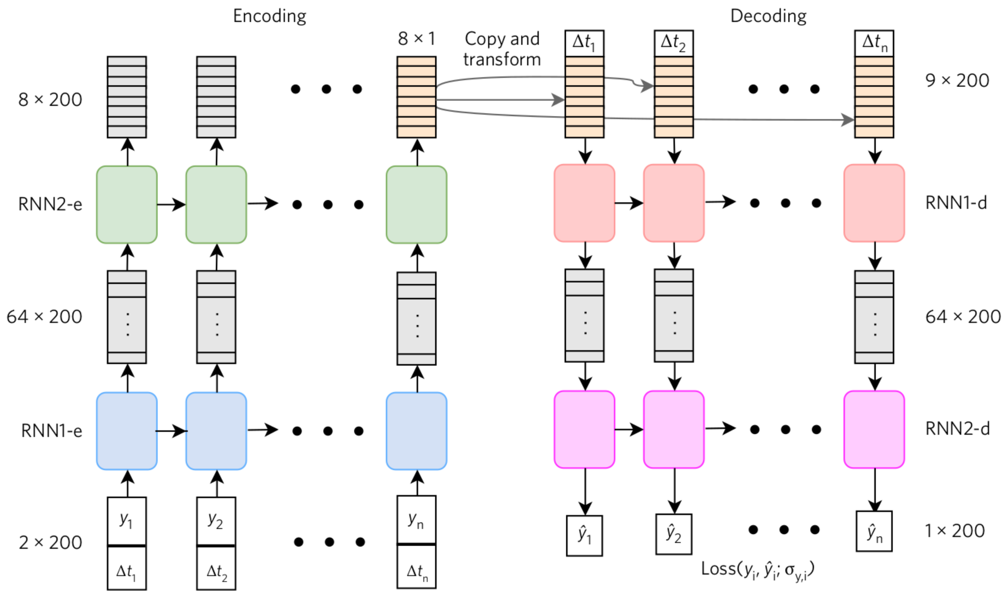
2.2.2. VRAE Including Delta Times

A VAE, as any other auto-encoder architecture, is composed of a tangled encoder and decoder models trained on an unsupervised scenario (unsupervised refers to the fact that no labels are used as inputs to the model). The encoder model q ϕ ( z | x ) , with parameters ϕ , codifies the input pattern x to a multi-dimensional latent variable z , which has fewer dimensions than the original space (data compression). The decoder model p θ ( x | z ) , with parameters θ , reconstructs the input pattern from the codification z . The objective of the model is to maximize a (variational) lower bound L ( θ , ϕ ; D ) of the log-likelihood ( θ , ϕ ; D ) [29]. For example, for an input pattern x , we have:
L ( θ , ϕ ; x ) = E q ϕ ( z | x ) log p θ ( x , z ) log q ϕ ( z | x ) L ( θ , ϕ ; x ) = E q ϕ ( z | x ) log p θ ( x | z ) D K L q ϕ ( z | x ) p θ ( z ) ,
where the first term of L is related to the expected reconstruction likelihood and the second enforces the consistency between the posterior obtained by the encoder q ϕ ( z | x ) and some prior p θ ( z ) , based on the Kullback–Leibler (KL) divergence [38]. In the standard VAE, the distribution q ϕ ( z | x ) is typically normal, N μ ( x ) , diag ( σ ( x ) ) , where μ ( x ) and σ ( x ) are modeled with neural networks yield vectors. However, the common choices of p θ ( z ) lead to a KL divergence that can be analytically integrated. However, the first term of L needs to be approximated with the so-called re-parametrization trick: z ^ = μ + σ ϵ , with an auxiliary noise variable ϵ N ( 0 , I ) . The operator ⊙ symbolizes the Hadamard product, i.e., an element-wise product of vectors and matrices.
The fully connected VAE for light curves proposed by [35] could be extended to adapt RNN models into the encoder q ϕ ( z | x ) and decoder p θ ( x | z ) as a VRAE model. However, to adapt the model to incorporate the time information of the light curves, we need the time intervals ( δ ) as an extra input channel. To do this, we followed the idea of the RAE t architecture proposed by Naul et al. [10] (shown in Figure 2), which adds the time information in both encoding and decoding sections of the auto-encoder. The proposed extension is named VRAE t model (VRAE plus time information). This model could be expressed by the encoder q ϕ ( z | x , δ ) and the decoder p θ ( x | z , δ ) , which have the time information δ of every observation on the time series x as an extra input signal.
The motivation behind the variational extension is that the generative (stochastic) model learns a latent variable with smoother transitions, meaning that their latent space must be continuous [29]. Furthermore, since the model learns the distribution of the encoded variable, it becomes robust to input variations, similarly to a denoising auto-encoder [31]. Indeed, the learned distribution must have more likely regions or confidence intervals where the input data should be.

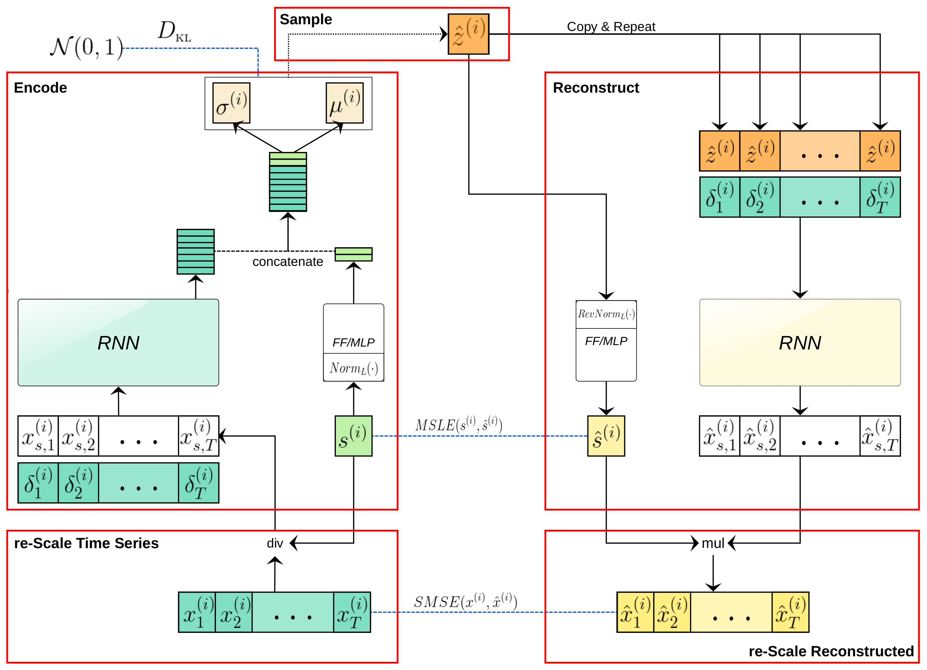
2.2.3. VRAE with Embedded Re-Scaling

Currently, deep learning methods need a standardized version of the input representation x ( i ) that retains the original distribution but re-scaled to more tractable magnitudes. This is used for properly training neural network models, based on the generalization principle that magnitudes of weights and activation functions must be somehow bounded [39,40]. Furthermore, Ioffe & Szegedy [41] recommend that a normalization step is added after each layer to obtain more stable training. On a time series, this transformation is usually based on its own magnitude behavior, e.g., the range, standard deviation, and norm. For example, x ( i ) = ( x ( i ) min ( x ( i ) ) ) / ( max ( x ( i ) ) min ( x ( i ) ) ) change the range magnitudes to [ 0 , 1 ] , or x ( i ) = ( x ( i ) mean ( x ( i ) ) ) / std ( x ( i ) ) could lead to x ( i ) N ( 0 , 1 ) if x ( i ) is normally distributed. These transformations are necessary for the model to detect pattern behaviors instead of magnitude behaviors. The problem is that the information on the original scale of variability is lost in the process, which can be useful in some cases. Focused on light curves, we propose adding the Flux standard deviation s ( i ) of the flux time series x ( i ) as an additional input to the VRAE t model, but still use the re-scaled version of the data for achieving bounded weights and activations. To the best of our knowledge, this is the first approach to do this as a end-to-end architecture.
We consider the F-std s ( i ) (Section 2.2.1 for problem notation) as another input pattern of the auto-encoder model VRAE t that also needs to be reconstructed. With this, the objective of the VRAE t with re-scaling or S-VRAE t is to reconstruct the time series on the un-scaled values, based on the F-std.
S-VRAE t architecture: The outline of the main components of the S-VRAE t model which clarify the differences with respect to VRAE t , as summarized here:
  • Re-scale data: The first layer of the encoder q ϕ ( · ) re-scales the data by dividing on the F-std. This step is performed in order to use the standardized version of the data, as the literature recommends.
  • Encode: The encoder q ϕ ( · ) adds the F-std as an input pattern to the coding task by q ϕ ( z ( i ) | x ( i ) , δ ( i ) , s ( i ) ) = N ( μ ( i ) , diag ( σ ( i ) ) ) in order to extract the information on it.
  • Sample: The sampled latent variable is given by: z ^ ( i ) = μ ( i ) + σ ( i ) ϵ , with ϵ N ( 0 , I ) .
  • Reconstruct: The decoder p θ ( x ( i ) | z ( i ) , δ ( i ) ) adds the F-std to the reconstruction task in order to estimate the original F-std by p θ ( s ( i ) | z ( i ) ) .
  • Re-scale reconstruction: The last layer of the decoder re-scales the data, by returning the reconstructed F-std (multiplied by it). This final step is performed in order to obtain a reconstructed time series on the un-scaled values’ representation.
Based on the high variability in the range of values of the F-std and inspired by [41], we introduced a normalization logarithm layer ( N o r m L ) that is applied to s ( i ) . Considering a random variable a, the forward pass to obtain a new value b is given by
b = N o r m L ( a ) = log a mean ( log a ) std ( log a ) .
The mean and standard deviation ( std ) are previously computed over the whole dataset. Furthermore, another layer is introduced to reverse this transformation, given by
a = R e v N o r m L ( b ) = exp b · std ( log a ) + mean ( log a ) = N o r m L 1 ( b ) .
Compared against the VRAE t on Algorithm 1, a pseudo-code of the S-VRAE t forward pass is presented on Algorithm 2. Here, it can be seen that the main differences are the re-scaling process inside the model and the additional input pattern to be used. The first thing to formalize is that g w ( · ) and f w ( · ) are non-linear functions (i.e., deep learning models) parameterized by the weights w. The E ( · ) , which stands for the embedding function, corresponds to the first layers of a deep learning model. Inside f ϕ ( · ) , the E 1 ( · ) is an RNN model and E 2 ( · ) is a multi-layer perceptron (MLP) model with N o r m L ( · ) as the first layer. Here, E 1 ( · ) codifies the information from the noisy standardized time series, while E 2 codifies the F-std. On the decoder phase, the g θ 1 ( · ) is similar to a mirror model of E 1 ( · ) , while reversing what E 2 ( · ) does, the last layer of g θ 2 ( · ) is R e v N o r m L ( · ) . Then, g θ 1 ( · ) reconstructs the standardized version of the time series and g θ 2 ( · ) reconstruct the F-std.
The architecture of the proposed S-VRAE t is illustrated in Figure 3. Please note that the Encode and Reconstruct blocks are the same as the RAE t in Figure 2 but without the F-std transformations. In summary, S-VRAE t learns a coded deep representation of the noisy un-scaled time series in an unsupervised way. The advantage is that those features are optimized for the specific input behavior (rather than classification) and are more disentangled (more independent between each other) than human-crafted counterparts. The evidence for this claim can be found in Section 3.3.
Algorithm 1 Forward pass VRAE t .
Input: x s ( i ) — scaled measurements of the time series
      δ i ) — delta times of the time series
Output: x ^ s ( i ) — reconstructed scaled time series
1:
// Encode to distribution:
2:
μ ( i ) f ϕ 1 E 1 ( x s ( i ) , δ ( i ) )
3:
σ ( i ) f ϕ 2 E 1 ( x s ( i ) , δ ( i ) )
4:
ϵ N ( 0 , I ) // Auxiliary noise
5:
z ^ ( i ) μ ( i ) + σ ( i ) ϵ
6:
// Decode or Reconstruct:
7:
x ^ s ( i ) g θ 1 z ( i ) , δ ( i )
Algorithm 2 Forward pass S-VRAE t .
Input: x ( i ) — measurements of the time series
      δ ( ) — delta times of the time series
Output: x ^ ( i ) — reconstructed time series
1:
s ( i ) std ( x ( i ) ) // F-std
2:
x s ( i ) x ( i ) s ( i ) // Step-1
3:
// Encode to distribution: Step-2
4:
μ ( i ) f ϕ 1 E 1 ( x s ( i ) , δ ( i ) ) , E 2 ( s ( i ) )
5:
σ ( i ) f ϕ 2 E 1 ( x s ( i ) , δ ( i ) ) , E 2 ( s ( i ) )
6:
ϵ N ( 0 , I ) // Auxiliary noise
7:
z ^ ( i ) μ ( i ) + σ ( i ) ϵ // Step-3
8:
// Decode or Reconstruct: Step-4
9:
x ^ s ( i ) g θ 1 z ( i ) , δ ( i )
10:
s ^ ( i ) g θ 2 z ( i )
11:
x ^ ( i ) x ^ s ( i ) · s ^ ( i ) // Step-5
In any VAE model, the objective of learning the distribution of the latent variable is to obtain the more likely reconstructed input pattern. In our S-VRAE t , the time series is reconstructed on the original un-scaled behavior x ^ ( i ) , so we can consider it as a smoothing or denoising model in a data-dependent way (based on data behavior). As the model processes the F-std inside it, it allows a robust F-std reconstruction (based on the noise). For example, consider the following decomposition of a time series: x ( i ) = x p ( i ) + n ( i ) , with x p ( i ) , flux measurements with an isolated or perfect environment such as the one modeled by [3], and n ( i ) as the intrinsic noise of these measurements, both with zero mean. Based on this decomposition, we can express the noised and denoised dispersion, F-std, as s n ( i ) = std ( x p ( i ) + n ( i ) ) and s p ( i ) = std ( x p ( i ) ) , respectively. The denoised F-std s p ( i ) could only be close-estimated by S-VRAE t in order to re-scale the denoised reconstructed time series x ^ p ( i ) = x ^ p , s ( i ) · s p ( i ) (Step 5 of Algorithm 2). Other models, with a fixed re-scaling process, will always use the noised F-std: s n ( i ) . This shows the capacity of S-VRAE t to learn to smooth an un-scaled time series.

2.2.4. Loss Function

In this section, we describe the optimization objectives of the proposed variational auto-encoder models (VRAE t and S-VRAE t ) for the time series domain.
Reconstruction loss: We used a modified version of the mean squared error (MSE) function for the un-scaled variable time series, named weighted or re-scaled MSE, given by
SMSE ( X , X ^ ) = 1 N i = 1 N w ( i ) · 1 T i j = 1 T i x j ( i ) x ^ j ( i ) 2 ,
where the additional weight w ( i ) is associated to every input pattern (as a sample weight [42]) and is defined as the inverse of the variance in the time series: w ( i ) = ( var ( x ( i ) ) ) 1 . The weight value comes from w i = ( s ( i ) ) 2 , with the idea of normalizing and removing the intrinsic dispersion of the time series x ( i ) , and so every input pattern has the same impact in the objective (note that SMSE is similar to the chi-square error of a linear least-squares fit with (uncorrelated) uncertainties that follows from a maximum likelihood approach). In order to perform a proper reconstruction of the input patterns, the SMSE is applied as a loss function for the deterministic counterpart of VRAE t , i.e., the RAE t model.
Variational loss: The two factors to optimize on the variational lower bound (Equation (1)) could be expressed by: (i) a reconstruction factor through the SMSE described above; and (ii) the closed solution for the KL divergence with normal priors [29]. Following Higgins et al. [43], we combine these two factors using a regularization parameter β obtaining the loss function of the VRAE t model:
V ( X , X ^ ) = SMSE ( X , X ^ ) + β · D K L Z N ( 0 , I ) .
Our earlier experiments on the validation set led us to set the β hyper-parameter to a small value of 10 3 . This means that the priority is set on the reconstruction task but with a variational component of regularization.
Variational loss with re-scaling: As our proposed S-VRAE t adds the F-std to the reconstruction task, we need to specify an additional loss that guides this reconstruction. We used the mean squared logarithm error (MSLE) as a loss function, given by
MSLE ( S , S ^ ) = 1 N i = 1 N log s ( i ) log s ^ ( i ) 2 .
Then, the learning objective of the S-VRAE t model is given by
SV ( X , S ) , ( X ^ , S ^ ) = V ( X , X ^ ) + α · MSLE ( S , S ^ ) ,
where the α hyper-parameter was set to 10 1 / var ( log S ) . The same motivation used for β led to set the 10 1 value, firstly giving relevance to the reconstruction loss SMSE inside V. However, the var ( log S ) value is to re-scale the values of the MSLE loss (by removing the standard deviations) to the same proportions of SMSE loss. The loss function used helps the models, guiding them into the right reconstruction. As each component has a hyper-parameter weight, this does not force the model to explicitly predict the exact value, as it only acts as a data-driven loss.

3. Experimental Setup and Results

This section presents the experimental setup in which the proposed methods were validated and the results obtained through that setup.

3.1. Dataset

Our work used the Kepler Objects of Interest (KOI, [44]) dataset described by the NASA Exoplanet Archive [45]. It is composed of 8054 light curve records (https://archive.stsci.edu/kepler/koi/search.php accessed on 20 September 2019) where every KOI describes a target star in the field of view that exhibits transit-like signatures in its light curve. Primarily, a TCE that was accepted as a valid astrophysical signal based on the diagnostic tests described in [44] was designated as a KOI. According to the NASA Exoplanet Archive (https://exoplanetarchive.ipac.caltech.edu/ accessed on 10 July 2021), KOIs are categorized into three tags: Confirmed, claimed exoplanets through extensive scientific analysis and follow ups; False Positive, evidence indicates that they correspond to another type of behavior not associated with transit exoplanets (e.g., eclipsing binary systems), and Candidate, those that are still under study (unlabeled data). In some cases, multiple KOIs are obtained from the analyzed host star, where each object contains the raw flux measurements with the timestamps (in BKJD), including the instrumental error associated with each measure. The time unit Barycentric Kepler Julian Day (BKJD) corresponds to BKJD = BJD 2454833 , while the Barycentric Julian Day (BJD) is simply Julian days (the continuous count of days since the beginning of the Julian period) with some corrections based in the Earth’s position and the barycenter of the Solar System. The long-cadence sampling rate of the 4-years’ worth of measurements was 0.0204 BKJD on average (i.e., half an hour); however, there is 22.98% of missing values on average in the collected and used light curves. The light curve data [46,47,48] described here may be obtained from the Mikulski Archive for Space Telescopes (MAST) (https://dx.doi.org/10.17909/T9RP4V accessed on 10 July 2021).
The archive also provides a set of metadata values (https://exoplanetarchive.ipac.caltech.edu/docs/API_kepcandidate_columns.html accessed on 10 July 2021), some of which (usually those related to the host star such as its effective temperature and metallicity) are cross-matched from other catalogs, while others are calculated following a Mandel–Agol modeling fit [3] according to LS and MCMC. For comparing our self-generated features with model-based ones, we selected those that could be obtained from the light curves based on the modeling, which are: Period; First Transit Time; Inclination; Planet Radius (over Stellar Radius); Semi-Major Axis (over Stellar Radius); Transit Duration; Impact Parameter; and Fitted Stellar Density. Furthermore, we included the Limb Darkening Coefficients (quadratic model) even though they are not solved –they are fixed in the fit for each star, but they are still involved in the modeling of the light curves.
For data pre-processing, we used a detrending process that also normalized the stellar flux and apriori removed low frequency noise. It combines ideas from the combined differential photometric precision proxy used by [49]—subtract polynomial fit and sigma-clipping, and the Argabrightening detection by [50]—subtract polynomial fit and subtract median filter. This detrending process was performed over the raw flux measurements by using time. It consists of applying and then subtracting a two-degree polynomial fit with a window of 151 points (approximate 3 days on Kepler), the Sav-Gol filter [51]. Then, it subtracts a moving median filter with a window of 25 points. Finally, during the sigma-clipping, we remove positive outliers that are greater than 5 σ and remove negative outliers less than 40 σ .

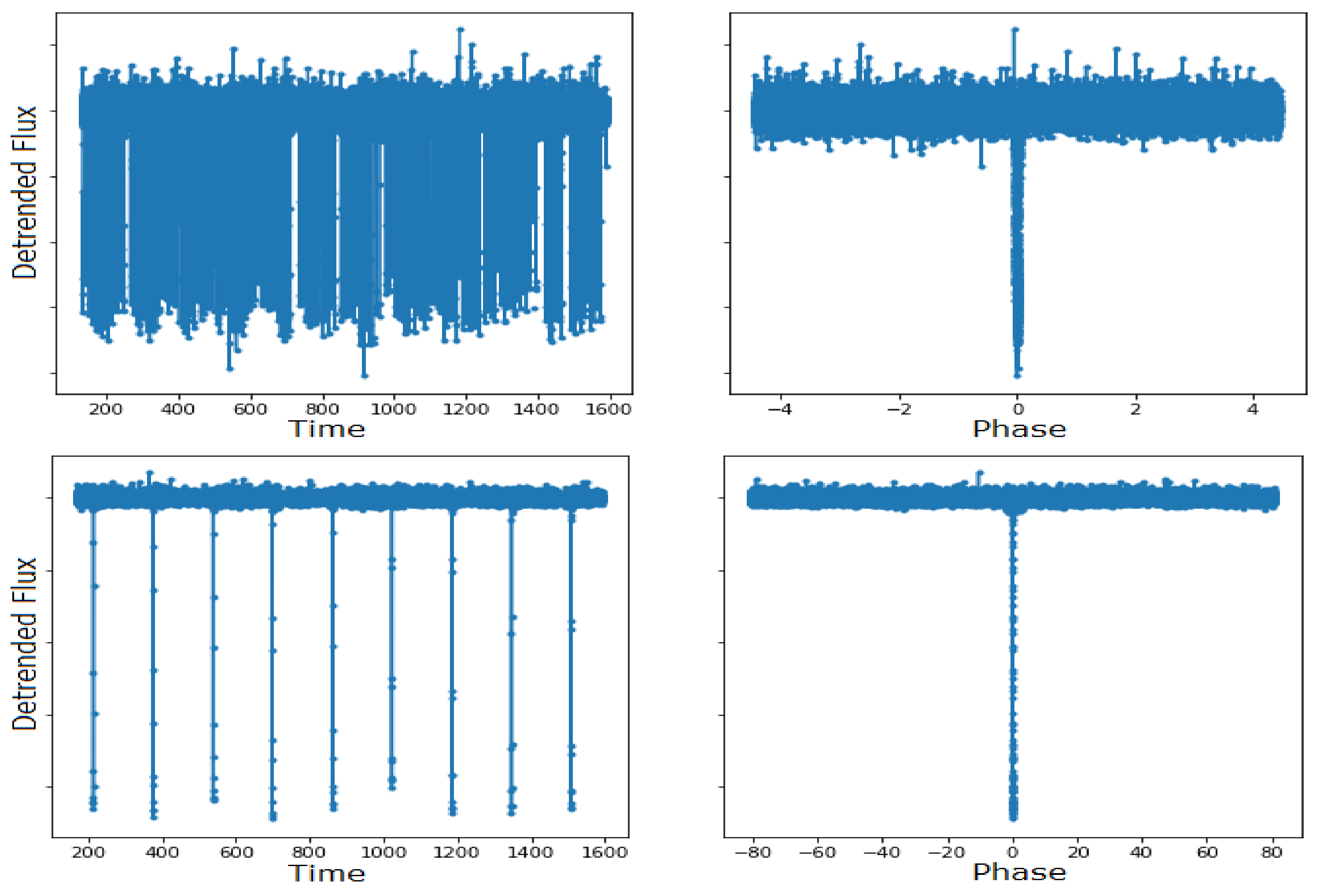
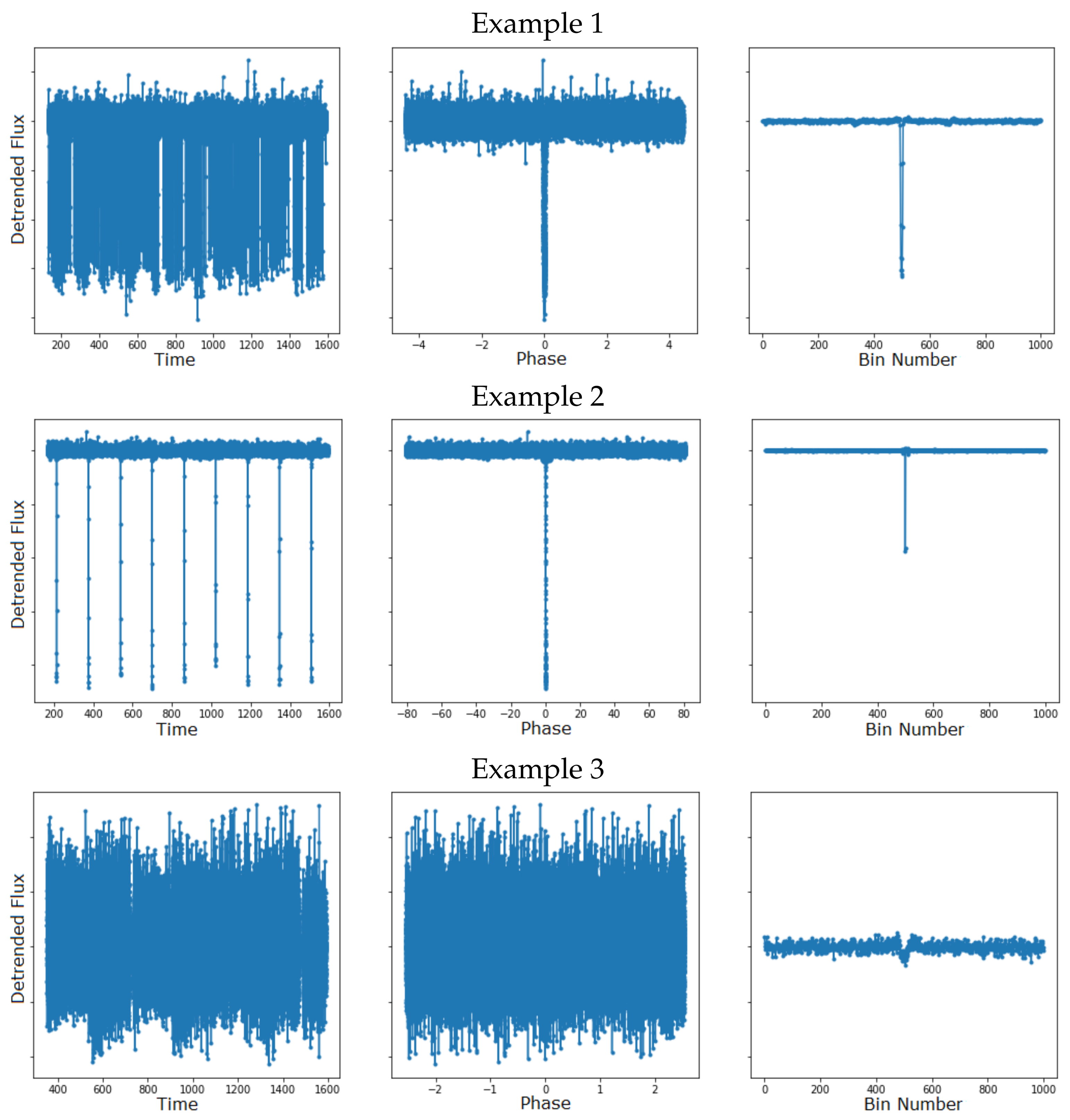
3.1.1. Data Representation

For the detrended flux light curve f ( i ) , we used the global-folded representation proposed by Shallue & Vanderburg [6]. First, it produces p ( i ) , a vector with the same number of points by folding the detrended light curves on the period (P with the event centered (fold step). Then, a median window was applied every P / T times over the folded light curve p ( i ) (global step) producing x ( i ) , a vector with T points (empty values masked with 0) such that each light curve has the same length with the width interval depending on the period P. The parameter T controls the trade-off between a detailed representation and having enough points on each window for the median to be meaningful.
Figure 4 shows examples of folded and global-folded representations of some light curves (based on Kepler). The second example illustrates a general disadvantage of this method, where long-period KOIs may end up with very narrow transits that fall entirely within a small number of bins. On the other hand, the third example shows how the global-folded representation helps obtain a cleaner version of the light curve when the planets are small.
As explained in Section 2.2, the delta times ( δ ( i ) ) of x ( i ) are considered as an additional input for the learning models. Furthermore, please recall that the measurements of the global-folded light curve x ( i ) were previously scaled through x s ( i ) = x ( i ) s ( i ) for VRAE t , while the proposed S-VRAE t model directly uses the un-scaled global-folded light curve x ( i ) .

3.1.2. Data Selection and Augmentation

We set a data-driven mask over all the objects (labeled and unlabeled) of the KOI data (8054 records) to filter out light curves without a transit behavior, obtaining 4317 objects to train in an unsupervised fashion. The process is described below:
  • Check for Kepler flags (in the metadata) and remove objects with “secondary event” or “not transit-like” flags;
  • Remove objects with a “transit score” (in the Kepler metadata) less than 0.55 ;
  • Perform a Mandel–Agol fit and remove objects with (SMSE) residual greater than 1.
The candidate objects that are not transits (“not transit-like” flags) could be because the detection was from instrumental artifacts errors, non-eclipsing variable stars or another object (non-planetary) in the background. On the other hand, the objects with a statistically different secondary event (“secondary event” flag) are most likely caused by an eclipsing binary system, i.e., two stars orbiting around their barycenter.
Furthermore, as a data augmentation step, we doubled this dataset by mirroring each folded light curves [52]. This represents of the same object, with the same properties, orbits the star in the opposite direction.

3.2. Model Assessment and Implementation

For assessing the quality in the latent representation of global-folded light curves learned by the proposals, we propose validating the reconstruction task based on that representation, the representation disentanglement, and the true planet classification by using the representation (extrinsic validation).

3.2.1. Reconstruction Validation

Using the encoder–decoder architecture, we assessed the reconstruction task by comparing the estimated input pattern x ^ and real value x using the root mean squared error (RMSE) and mean absolute error (MAE) as performance metrics. For evaluating the denoising effect on the reconstruction, we used the estimated input pattern x ^ and measure the auto-correlation (Auto-C) and the mean of the differences (Diff-M) between consecutive values. A high Auto-C and low Diff-M, is associated with a smoother time series. For measuring the structure left within the residual noise (difference between real and estimated time series), we used an information theory score called spectral entropy (Spectral-H) [53]. A high value of this entropy means a less structured residual in terms of signal frequencies.
Smoothing a time series is a classical signal processing task. Unfortunately, this is not straightforward for transits because transits are (statistically speaking) isolated behaviors or anomalies as shown in Figure 4. Therefore, a standard denoising model will remove transits by considering them anomaly deviations of the “normal” stellar flux. Based on this, we selected the following signal processing baselines to compare our models: the Butterworth passband filter [54], a moving average filter with different window sizes, and the RAE t [10]. In addition, we performed a Mandel–Agol (M-A) fit over the global-folded light curves, modeling points on the phase-space of this representation. The M-A fit was performed to obtain a reasonable time period for the exoplanet population analysis, using the same model calculation given by Kepler. This was implemented using the ktransit library [55] with an LS optimization based on a quadratic limb darkening model and the star coefficients of the Kepler metadata, given by [56]. At this point, the LS optimization hyper-parameters were set to the library defaults.
To make a fair comparison, the initial estimate for the period and mid-transit time was the same as that used in the folding of the light curves.

3.2.2. Disentanglement Validation

Using the encoder sub-architecture, we analyzed the disentanglement of the latent representation based on the features’ dependency. To perform this in an unsupervised way [36], we used the Pearson correlation between all the features on the representation to determine how orthogonal the generated features are. We report the average over all the values (Pcorr) and the average over the absolute values (Pcorr-A). The mutual information (MI) between the continuous features was also measured, including a normalized version (of a value in the range [ 0 , 1 ] ) that is obtained by dividing on the entropy of every feature (N-MI). The calculation of MI is a discrete approximation of the real continuous space calculation, based on the k-neighbors’ implementation [57].
Here, we compare the high-level specialized features included in Kepler’s metadata with the features learned by RAE t [10] and the PCA features extracted over the frequency domain (spectrum) representation of the time series (Fourier followed by PCA or F-PCA) [20].

3.2.3. Classification Validation

Using the latent representation learned by the encoder sub-architecture, we analyzed the performance in a binary classification task (is the object a true exoplanet?). This is an extrinsic assessment of the quality of the representation since the model did not have learning as a specific objective (task-free). The classification was made using an MLP model built over the representation with 128 units and relu activation, ending with a sigmoid classification layer (one-unit) as output. The dataset labels were used to carry out this evaluation, with 2281 exoplanets and 3976 non-exoplanets (1797 of the KOIs are unlabeled, i.e., candidates). The network is trained in 70% of the labeled data with 30% remaining as a test set. The best parameters found over 200 epochs are stored (with 128 batch size). As the dataset contains a larger number of non-exoplanet objects (in an unbalanced scenario), an F 1 score macro averaged ( F 1 -Ma) criterion was used to assess the results, where a high value means high precision and recall simultaneously on both classes.

3.2.4. Model Implementation

Following the RAE t model [10], the recurrent layers of our models implement GRU over the widely known long short-term memory (LSTM, [58]) as it presents roughly the same performance [59], but has fewer parameters and needs to store less information per time (i.e., it is faster). The encoder and decoder recurrent blocks of the models (i.e., E 1 ( · ) and g 1 ( · ) on Algorithms 1 and 2) are a stack of two bidirectional RNN layers of 64 units in order to increase representation complexity as [10] presented. The models were trained for 300 epochs with a batch size of 64 and an Adam optimizer [60]. The implementation was performed using the Keras library (https://keras.io, accessed on 10 July 2021).

3.3. Results

The following results were obtained at the Chilean Virtual Observatory (ChiVO) datacenter [61] on an Intel Xeon CPU E5-2680 2.50 GHz with 12 cores and 64 GB of RAM. For the experiments, we set T = 300 and the dimension of the encoder representation D to 16, generating 95% compression. The results correspond to just one sample set. All the implementations are available in our repository (Github, accessed on 12 October 2021).

3.3.1. Is the Time Needed?

Table 1 shows the results on the behavior of the model when using the time information. The first thing to mention is that the learning models, on average, manage to reconstruct the data without the time channel. However, including the delta time channel as input to both sub-architectures (encoder and decoder) helps the methods to regularize the reconstruction. This phenomenon can be seen by the RMSE and MAE metrics since they report an increase when using time, while the Spectral-H indicates that the models leave more noise in the residual reconstructing non-uniform patterns of the original time series. In that sense, the denoising results report that the consecutive values of the reconstructed time series are more auto-correlated and with smoother transitions. All this indicates that the model does not focus on exactly imitating each measurement but generates smoother light curves with more residual noise. This effect is stronger on the RAE t model, since the variational loss on VRAE t already forces some regularizations.

3.3.2. Quality Evaluation

The reconstruction and smoothing scores for different methods and configurations are presented in Table 2. As expected, passband methods offer a very good denoising behavior, but fail to properly reconstruct the signal. For example, if we vary the filter on the passband, by specifically narrowing the pass frequency, the reconstruction error increases and becomes smother (high Auto-C and low Diff-M). The same effect occurs for the moving average method when we increase the window size. Compared to the passband, the moving average method presents smaller reconstruction errors but producing a rougher time series (low Auto-C). The Mandel–Agol fit has a smaller reconstruction error compared to the passband and moving average methods, which is because it performs a specific and specialized problem fit (transit light curves). The simulation function does not consider factors of smoothness, as it models the ideal behavior of the transit objects. Nevertheless, the auto-correlation is still strong as in the previous methods, with the smallest difference on consecutive values.
It is clear that the learning-based methods (auto-encoders), due to data learning, have the lowest reconstruction errors only comparable with a moving average with a window size of 3. Furthermore, the reconstructed data are still significantly smoother than those of the original time series (denoising effect). Between them, variational proposals have a greater auto-correlation (i.e. smoother) than their deterministic counterpart RAE t . Except for the Mandel–Agol fit and the narrowest passband, they have the smallest difference on consecutive values (Diff-M), showing smoother transitions in the local behavior of the time series.
If we take a look at the spectral entropy of the residual, we clearly identify that learning-based methods exhibit the best scores. This means that these methods really focus on learning the time series patterns to perform the reconstruction instead of removing structure for achieving high smoothness as in the generic denoising methods presented. Please note that the spectral entropy has a reference value of 0.840 (i.e., on the original light curve) and its maximum value is 1.000 (i.e., a uniform distribution of frequencies).
Figure 5 shows a few examples of reconstructed light curves for a better understanding of the previous results. The RAE t approach tends to keep the noise on the edges of the time series (in order to perform a good reconstruction), while our proposal (S-VRAE t ) generates a smoother transit to the extent of being comparable with the M-A transit model, removing more high-frequency noises, as can be seen in the figure. The VRAE t model is not shown because visually it is quite similar to S-VRAE t . On the other hand, the Mandel–Agol model residuals show that the reconstruction errors are related to the positive values, as the function models that the measured light could not be greater than the regular/normal star’s light intensity (without objects in front of the observer), i.e., it is limited by the model itself.
In Table 3, we present the disentanglement of the representation based on the feature dependence. Here, it can be seen that learning-based methods (AEs) obtain features with less information duplicity than the metadata features obtained by Kepler, i.e., the learned features are more disentangled. Minimizing the correlation and mutual information could simplify the task of identifying independent linear and non-linear processes in the system, respectively.
We computed an F-PCA representation from the whole (unfolded) raw measurements and from the folded representation. Both obtained components were linearly independent between them based on the orthogonality of the PCA formulation. However, the F-PCA method over the fold representation produces less MI, as an example of optimal independence for the problem. The closer values to F-PCA (in the folded curve) are from the proposed model with re-scaling (S-VRAE t ) showing the good impact of including the F-std into the model. It is worth noting that the variational proposed models (VRAE t and S-VRAE t ) learn a space with more independent components (linearly and based on mutual information) than the deterministic counterpart RAE t .

3.3.3. Application of the Learned Representation

An extrinsic way to assess the quality of a representation is to impose a task: in this case, classifying candidate light curves as true exoplanets (Confirmed) or another variability (False Positive).
Table 4 presents the results of this binary classification. Here, we compare different representations, including the auto-encoders and supervised methods from the global-folded light curve shape (with T = 300 bins). The “1D CNN” is a supervised method that extracts features based on convolutions, while “RNN t ” does it based on recurrence, both with the classification layer mentioned in Section 3.2.3 on top. The 1D CNN network architecture is inspired by [6], until the third convolutional block using only the global view on this KOI dataset (a subset of the TCE). While the RNN t architecture is the recurrent encoder of RAE t /VRAE t without the decoder phase.
In Table 4, it can be seen that the representation of the variational extension (VRAE t ) gives an improvement on all the classification metrics with respect to the RAE t representation, as well as being better than the other unsupervised methods. This can be explained due to the generalization capacity of the implemented latent variables within the variational model. Furthermore, the results of the S-VRAE t suggest that the method succeeds in using the Flux standard deviation of the light curve, as it is able to codify better patterns in the representation to distinguish in the classification task. Indeed, the S-VRAE t representation has the best classification performance among unsupervised techniques on all the metrics, being quite close to the supervised ones. This indicates that, without access to labels, we are obtaining a representation almost as good as the supervised method on that task and at the same time, useful in other factors.

4. Discussion

In Section 3.3.1, we show that the time is needed if a regularization effect and smoothing is desired. We briefly discuss the reasoning behind why time could contribute to phase-space light curves. As [10] introduced, the time information is not only used as input in the first stage (encoder process), as the decoder process needs the space reference where to reconstructs it. Each light curve has its own phase-space based on its period, then the delta times of the bins for different light curves will be different. Even if the delta times are similar for some light curves, the decoder does not know that information. The model will have to learn to reconstruct in each phase-space, since the decoder processes the previous time and its memory with a recurring operation. By having the same vector z ^ repeated at each time-step in the first decoder layer (Figure 3), the temporal information of each point for the different light curves could be beneficial in the reconstruction.
Section 3.3.2 shows that the proposed methods offer a good combination of reconstruction and denoising of the light curves. In addition, adding the re-scaling into the model (S-VRAE t ) seems to produce a smoother reconstructed time series but with the cost of increasing the reconstruction error, but both results are quite similar. The disadvantage in reconstruction is expected because the model needs to learn to simultaneously codify and reconstruct the F-std of the data. These results indicate that the representation learned by the variational proposals allow a smoother version of the light curve reconstruction that is the most similar (except for RAE t ) to the original curves, these being the methods that perform the best removal of unstructured patterns (noise) on the light curves among all the methods. While the results in Table 3 illustrate that more exclusive information could be stored through the learned variational features of the proposed models (as every feature represent a more different structure) and used for different proposes, as shown in the following. In addition, as shown in [36], a more disentangled representation indicates that the features found are closer to the underlying factors that explain the data behavior.
The unsupervised feature extraction methods are useful based on the classification improvement over the raw global-folded representation, as shown in Section 3.3.3. This suggests that it is easier to discriminate using these compact representations than the raw folded measurements (95% compression). In addition, the 16-dimensional representation is computationally lighter, taking a fraction of the time to train the supervised network (i.e., 10%). However, supervised methods that train an internal representation explicitly specialized for the task have better classification results over all unsupervised techniques. This is expected if we take a look at the input mapping for the desired output y with a classification model C ( · ; w ) parameterized by w. For example, (considering that the input x should be ( x , δ ) ), the VRAE t will estimate y ^ = C ( f ( x ; ϕ ) ; w ) by learning w with ϕ fixed, since the representation μ = f ( x ; ϕ ) is already learned (in the unsupervised auto-encoder objective without knowing y). However, the supervised version of this method (RNN t ) will estimate y ^ by learning ϕ as well (in the supervised objective knowing y). Despite this, it is worth noting that our proposed S-VRAE t achieves a performance quite close to the maximum model capacity for this specific task (RNN t ) by learning ϕ without labels (y). In this case, we refer to the capacity to extract the information from the input x , and it would be given by the structure of f ( x ; ϕ ) , e.g., a linear function or not, in the case of a neural network, the architecture, or how ϕ is organized within the network.

5. Conclusions

In this work, we used variational (stochastic) auto-encoder models to learn quality deep representations for global-folded transit light curves. We focused on adapting the variational auto-encoders to properly include the time information as delta times outperformed all of their deterministic competitors. We presented two methods, one of which included a re-scaling pre-processing of time series (as an end-to-end architecture) which led to significant improvements on different quality evaluation schemes that we proposed.
The evaluation of the learned representation showed that the variational proposals obtain a better quality. This means that the representation is: (i) more informative, i.e., more independent features, so more information could be stored; (ii) more useful, i.e., more effective for the classification of exoplanets; and (iii) more robust, i.e., learn a smoother light curve reconstruction. By adding the re-scaling into the model, these three effects increase. For example, the S-VRAE t model ends up being almost as informative as the optimal PCA, at the same time that it produces a denoising effect on the reconstruction that is visually comparable to a Mandel–Agol fitted model. Furthermore, the model achieves a classification performance quite close to its maximum model capacity.

Future Remarks

Future work includes performing a sensitivity analysis on the architecture parameters. Furthermore, we believe that interpreting these informative, useful, and robust features by mapping each dimension to an astronomical concept could enrich current knowledge about orbiting objects. Furthermore, this could be a useful tool for characterizing exoplanets and identifying non-conventional planetary properties, such as magnetic bow shocks, exomoons, or exorings. Another exciting line of study considers the use of the S-VRAE t model to help elucidate which characteristics of a transit model are most relevant. With this, we could generate new synthetic transit light curves and face other learning tasks such as classification problems.

Author Contributions

F.M.: conceptualization, methodology, software, validation, formal analysis, visualization, writing—original draft, writing—review and editing; P.O.: methodology, software, formal analysis, writing—original draft, writing—review and editing; M.B.: conceptualization, writing—original draft, writing—review and editing, visualization; G.M.: data curation, writing—review and editing; M.A.: conceptualization, project administration, funding acquisition, supervision, resources. All authors have read and agreed to the published version of the manuscript.

Funding

This research was funded by PIIC-DGIP of Universidad Técnica Federico Santa María, ANID-Basal Project FB0008 (AC3E) and ANID PIA/APOYO AFB180002 (CCTVal).

Institutional Review Board Statement

Not applicable.

Informed Consent Statement

Not applicable.

Data Availability Statement

The data used in this work may have been obtained from the MAST: https://dx.doi.org/10.17909/T9RP4V accessed on 20 September 2019.

Acknowledgments

This work was possible thanks to the Chilean Virtual Observatory, ChiVO.

Conflicts of Interest

The authors declare no conflict of interest. The funding sponsors had no role in the decisions regarding the work and manuscript.

Abbreviations

The following abbreviations are used in this manuscript:
AEAuto-Encoder
Auto-CAuto-Correlation
BKJDBarycentric Kepler Julian Day
BJDBarycentric Julian Day
CRTSCatalina Real-Time Transient Survey
CNNConvolutional Neural Network
Diff-MMean of the Differences
F-PCAFourier plus PCA
GRUGated Recurrent Unit
KOIKepler Objects of Interest
LSLeast Squares
LSSTLegacy Survey of Space and Time
M-AMandel–Agol
MASTMikulski Archive for Space Telescopes
MAEMean Absolute Error
MCMCMarkov Chain Monte Carlo
MIMutual Information
MLPMulti-Layer Perceptron
MSEMean Squared Error
MSLEMean Squared Logarithm Error
NASANational Aeronautics and Space Administration
N-MINormalized MI
PCAPrincipal Component Analysis
PcorrPearson Correlation
Pcorr-APcorr in Absolute Values
RNNRecurrent Neural Network
RAERecurrent Auto-Encoder
RAE t RAE plus Time Information
S-VRAE t VRAE t with Re-Scaling
SMSERe-Scaled Mean Squared Error
RMSERoot Mean Squared Error
Spectral-HSpectral Entropy
TESSTransiting Exoplanet Survey Satellite
TCEThreshold-Crossing Event
VAEVariational Auto-Encoder
VRAEVariational Recurrent Auto-Encoder
VRAE t VRAE plus Time Information

References

  1. Tyson, J.A. Large Synoptic Survey Telescope: Overview. In Survey and Other Telescope Technologies and Discoveries; International Society for Optics and Photonics: Bellingham, WA, USA, 2002; Volume 4836, pp. 10–20. [Google Scholar] [CrossRef] [Green Version]
  2. Ricker, G.R.; Winn, J.N.; Vanderspek, R.; Latham, D.W.; Bakos, G.Á.; Bean, J.L.; Berta-Thompson, Z.K.; Brown, T.M.; Buchhave, L.; Butler, N.R.; et al. Transiting Exoplanet Survey Satellite. J. Astron. Telesc. Instrum. Syst. 2014, 1, 014003. [Google Scholar] [CrossRef] [Green Version]
  3. Mandel, K.; Agol, E. Analytic Light Curves for Planetary Transit Searches. Astrophys. J. Lett. 2002, 580, L171. [Google Scholar] [CrossRef] [Green Version]
  4. Moutou, C.; Pont, F.; Barge, P.; Aigrain, S.; Auvergne, M.; Blouin, D.; Cautain, R.; Erikson, A.R.; Guis, V.; Guterman, P.; et al. Comparative Blind Test of Five Planetary Transit Detection Algorithms on Realistic Synthetic Light Curves. Astron. Astrophys. 2005, 437. [Google Scholar] [CrossRef] [Green Version]
  5. McCauliff, S.D.; Jenkins, J.M.; Catanzarite, J.; Burke, C.J.; Coughlin, J.L.; Twicken, J.D.; Tenenbaum, P.; Seader, S.; Li, J.; Cote, M. Automatic Classification of Kepler Planetary Transit Candidates. Astrophys. J. 2015, 806, 6. [Google Scholar] [CrossRef] [Green Version]
  6. Shallue, C.J.; Vanderburg, A. Identifying Exoplanets with Deep Learning: A Five-planet Resonant Chain around Kepler-80 and an Eighth Planet around Kepler-90. Astron. J. 2018, 155, 94. [Google Scholar] [CrossRef]
  7. Pearson, K.A.; Palafox, L.; Griffith, C.A. Searching for Exoplanets using Artificial Intelligence. Mon. Not. R. Astron. Soc. 2018, 474, 478–491. [Google Scholar] [CrossRef]
  8. Schanche, N.; Cameron, A.C.; Hébrard, G.; Nielsen, L.; Triaud, A.; Almenara, J.; Alsubai, K.; Anderson, D.; Armstrong, D.; Barros, S.; et al. Machine-learning Approaches to Exoplanet Transit Detection and Candidate Validation in Wide-Field Ground-based Surveys. Mon. Not. R. Astron. Soc. 2019, 483, 5534–5547. [Google Scholar] [CrossRef]
  9. Mackenzie, C.; Pichara, K.; Protopapas, P. Clustering-based Feature Learning on Variable Stars. Astrophys. J. 2016, 820, 138. [Google Scholar] [CrossRef] [Green Version]
  10. Naul, B.; Bloom, J.S.; Pérez, F.; van der Walt, S. A Recurrent Neural Network for Classification of Unevenly Sampled Variable Stars. Nat. Astron. 2018, 2, 151–155. [Google Scholar] [CrossRef]
  11. Thompson, S.E.; Mullally, F.; Coughlin, J.; Christiansen, J.L.; Henze, C.E.; Haas, M.R.; Burke, C.J. A Machine Learning Technique to Identify Transit Shaped Signals. Astrophys. J. 2015, 812, 46. [Google Scholar] [CrossRef] [Green Version]
  12. Richards, J.W.; Starr, D.L.; Butler, N.R.; Bloom, J.S.; Brewer, J.M.; Crellin-Quick, A.; Higgins, J.; Kennedy, R.; Rischard, M. On Machine-learned Classification of Variable Stars with Sparse and Noisy Time-series Data. Astrophys. J. 2011, 733, 10. [Google Scholar] [CrossRef]
  13. Lomb, N.R. Least-Squares Frequency Analysis of Unequally Spaced Data. Astrophys. Space Sci. 1976, 39, 447–462. [Google Scholar] [CrossRef]
  14. Aguirre, C.; Pichara, K.; Becker, I. Deep Multi-survey Classification of Variable Stars. Mon. Not. R. Astron. Soc. 2019, 482, 5078–5092. [Google Scholar] [CrossRef]
  15. Tsang, B.T.H.; Schultz, W.C. Deep Neural Network Classifier for Variable Stars with Novelty Detection Capability. Astrophys. J. Lett. 2019, 877, L14. [Google Scholar] [CrossRef] [Green Version]
  16. Liu, W.; Wang, Z.; Liu, X.; Zeng, N.; Liu, Y.; Alsaadi, F.E. A Survey of Deep Neural Network Architectures and their Applications. Neurocomputing 2017, 234, 11–26. [Google Scholar] [CrossRef]
  17. Donalek, C.; Djorgovski, S.G.; Mahabal, A.A.; Graham, M.J.; Drake, A.J.; Fuchs, T.J.; Turmon, M.J.; Kumar, A.A.; Philip, N.S.; Yang, M.T.C.; et al. Feature selection strategies for classifying high dimensional astronomical data sets. In Proceedings of the 2013 IEEE International Conference on Big Data, Silicon Valley, CA, USA, 6–9 October 2013; pp. 35–41. [Google Scholar]
  18. Nun, I.; Pichara, K.; Protopapas, P.; Kim, D.W. Supervised Detection of Anomalous Light Curves in Massive Astronomical Catalogs. Astrophys. J. 2014, 793, 23. [Google Scholar] [CrossRef] [Green Version]
  19. Armstrong, D.J.; Pollacco, D.; Santerne, A. Transit Shapes and Self Organising Maps as a Tool for Ranking Planetary Candidates: Application to Kepler and K2. Mon. Not. R. Astron. Soc. 2016, 465, 2634–2642. [Google Scholar] [CrossRef] [Green Version]
  20. Bugueno, M.; Mena, F.; Araya, M. Refining Exoplanet Detection Using Supervised Learning and Feature Engineering. In Proceedings of the 2018 XLIV Latin American Computer Conference (CLEI), Sao Paulo, Brazil, 1–5 October 2018; pp. 278–287. [Google Scholar] [CrossRef]
  21. Mahabal, A.; Sheth, K.; Gieseke, F.; Pai, A.; Djorgovski, S.G.; Drake, A.J.; Graham, M.J. Deep-Learnt Classification of Light Curves. In Proceedings of the 2017 IEEE Symposium Series on Computational Intelligence (SSCI), Honolulu, HI, USA, 27 November–1 December 2017; pp. 1–8. [Google Scholar]
  22. Krizhevsky, A.; Sutskever, I.; Hinton, G.E. Imagenet classification with deep convolutional neural networks. Adv. Neural Inf. Process. Syst. 2012, 25, 1097–1105. [Google Scholar] [CrossRef]
  23. Lipton, Z.C.; Berkowitz, J.; Elkan, C. A Critical Review of Recurrent Neural Networks for Sequence Learning. arXiv 2015, arXiv:1506.00019. [Google Scholar]
  24. Rehfeld, K.; Marwan, N.; Heitzig, J.; Kurths, J. Comparison of Correlation Analysis Techniques for Irregularly Sampled Time Series. Nonlinear Process. Geophys. 2011, 18, 389–404. [Google Scholar] [CrossRef] [Green Version]
  25. Mondal, D.; Percival, D.B. Wavelet Variance Analysis for Gappy Time Series. Ann. Inst. Stat. Math. 2010, 62, 943–966. [Google Scholar] [CrossRef]
  26. Marquardt, D.; Acuff, S. Direct Quadratic Spectrum Estimation with Irregularly Spaced Data. In Time Series Analysis of Irregularly Observed Data; Springer: New York, NY, USA, 1984; pp. 211–223. [Google Scholar] [CrossRef]
  27. Che, Z.; Purushotham, S.; Cho, K.; Sontag, D.; Liu, Y. Recurrent Neural Networks for Multivariate Time Series with Missing Values. Sci. Rep. 2018, 8, 6085. [Google Scholar] [CrossRef] [Green Version]
  28. Cho, K.; Van Merriënboer, B.; Bahdanau, D.; Bengio, Y. On the Properties of Neural Machine Translation: Encoder-Decoder Approaches. arXiv 2014, arXiv:1409.1259. [Google Scholar]
  29. Kingma, D.P.; Welling, M. Auto-encoding variational bayes. arXiv 2013, arXiv:1312.6114. [Google Scholar]
  30. Fabius, O.; van Amersfoort, J.R. Variational Recurrent Auto-encoders. arXiv 2014, arXiv:1412.6581. [Google Scholar]
  31. Vincent, P.; Larochelle, H.; Lajoie, I.; Bengio, Y.; Manzagol, P.A. Stacked denoising autoencoders: Learning useful representations in a deep network with a local denoising criterion. J. Mach. Learn. Res. 2010, 11, 3371–3408. [Google Scholar]
  32. Guo, Y.; Liao, W.; Wang, Q.; Yu, L.; Ji, T.; Li, P. Multidimensional Time Series Anomaly Detection: A GRU-based Gaussian Mixture Variational Autoencoder Approach. In Proceedings of the Asian Conference on Machine Learning, Beijing, China, 14–16 November 2018; pp. 97–112. [Google Scholar]
  33. Park, D.; Hoshi, Y.; Kemp, C.C. A Multimodal Anomaly Detector for Robot-Assisted Feeding Using an LSTM-based Variational Autoencoder. IEEE Robot. Autom. Lett. 2018, 3, 1544–1551. [Google Scholar] [CrossRef] [Green Version]
  34. Xu, H.; Chen, W.; Zhao, N.; Li, Z.; Bu, J.; Li, Z.; Liu, Y.; Zhao, Y.; Pei, D.; Feng, Y.; et al. Unsupervised Anomaly Detection via Variational Auto-encoder for Seasonal KPIs in Web Applications. In Proceedings of the 2018 World Wide Web Conference, Lyon, France, 23–27 April 2018; pp. 187–196. [Google Scholar]
  35. Woodward, D.; Stevens, E.; Linstead, E. Generating Transit Light Curves with Variational Autoencoders. In Proceedings of the 2019 IEEE International Conference on Space Mission Challenges for Information Technology (SMC-IT), Pasadena, CA, USA, 30 July–1 August 2019; pp. 24–32. [Google Scholar] [CrossRef]
  36. Locatello, F.; Bauer, S.; Lucic, M.; Raetsch, G.; Gelly, S.; Schölkopf, B.; Bachem, O. Challenging Common Assumptions in the Unsupervised Learning of Disentangled Representations. In Proceedings of the International Conference on Machine Learning, Long Beach, CA, USA, 9–15 June 2019; pp. 4114–4124. [Google Scholar]
  37. Bengio, Y.; Courville, A.; Vincent, P. Representation Learning: A Review and New Perspectives. IEEE Trans. Pattern Anal. Mach. Intell. 2013, 35, 1798–1828. [Google Scholar] [CrossRef]
  38. Kullback, S.; Leibler, R.A. On Information and Sufficiency. Ann. Math. Stat. 1951, 22, 79–86. [Google Scholar] [CrossRef]
  39. Bishop, C.M. Neural Networks for Pattern Recognition; Oxford University Press: Oxford, UK, 1995. [Google Scholar]
  40. Montavon, G.; Orr, G.; Müller, K.R. Neural Networks: Tricks of the Trade; Springer: Berlin/Heidelberg, Germany, 2012; Volume 7700. [Google Scholar] [CrossRef]
  41. Ioffe, S.; Szegedy, C. Batch Normalization: Accelerating Deep Network Training by Reducing Internal Covariate Shift. In Proceedings of the International Conference on Machine Learning 2015, Lille, France, 6–11 July 2015; pp. 448–456. [Google Scholar]
  42. Freund, Y.; Schapire, R.E. A Decision-Theoretic Generalization of On-Line Learning and an Application to Boosting. In Proceedings of the European Conference on Computational Learning Theory, Barcelona, Spain, 13–15 March 1995; Springer: Berlin/Heidelberg, Germany, 1995; pp. 23–37. [Google Scholar] [CrossRef] [Green Version]
  43. Higgins, I.; Matthey, L.; Pal, A.; Burgess, C.; Glorot, X.; Botvinick, M.; Mohamed, S.; Lerchner, A. beta-VAE: Learning Basic Visual Concepts with a Constrained Variational Framework. Int. Conf. Learn. Represent. (ICLR) 2017, 2, 6. [Google Scholar]
  44. Thompson, S.E.; Coughlin, J.L.; Hoffman, K.; Mullally, F.; Christiansen, J.L.; Burke, C.J.; Bryson, S.; Batalha, N.; Haas, M.R.; Catanzarite, J.; et al. Planetary Candidates Observed by Kepler. VIII. A Fully Automated Catalog with Measured Completeness and Reliability Based on Data Release 25. Astrophys. J. Suppl. Ser. 2018, 235, 38. [Google Scholar] [CrossRef] [PubMed] [Green Version]
  45. Akeson, R.; Chen, X.; Ciardi, D.; Crane, M.; Good, J.; Harbut, M.; Jackson, E.; Kane, S.; Laity, A.; Leifer, S.; et al. The NASA Exoplanet Archive: Data and Tools for Exoplanet Research. Publ. Astron. Soc. Pac. 2013, 125, 989. [Google Scholar] [CrossRef] [Green Version]
  46. Stumpe, M.C.; Smith, J.C.; Van Cleve, J.E.; Twicken, J.D.; Barclay, T.S.; Fanelli, M.N.; Girouard, F.R.; Jenkins, J.M.; Kolodziejczak, J.J.; McCauliff, S.D.; et al. Kepler Presearch Data Conditioning I-Architecture and Algorithms for Error Correction in Kepler Light Curves. Publ. Astron. Soc. Pac. 2012, 124, 985. [Google Scholar] [CrossRef]
  47. Smith, J.C.; Stumpe, M.C.; Van Cleve, J.E.; Jenkins, J.M.; Barclay, T.S.; Fanelli, M.N.; Girouard, F.R.; Kolodziejczak, J.J.; McCauliff, S.D.; Morris, R.L.; et al. Kepler Presearch Data Conditioning II-A Bayesian Approach to Systematic Error Correction. Publ. Astron. Soc. Pac. 2012, 124, 1000. [Google Scholar] [CrossRef] [Green Version]
  48. Stumpe, M.C.; Smith, J.C.; Catanzarite, J.H.; Van Cleve, J.E.; Jenkins, J.M.; Twicken, J.D.; Girouard, F.R. Multiscale Systematic Error Correction via Wavelet-Based Bandsplitting in Kepler Data. Publ. Astron. Soc. Pac. 2014, 126, 100. [Google Scholar] [CrossRef]
  49. Gilliland, R.L.; Chaplin, W.J.; Dunham, E.W.; Argabright, V.S.; Borucki, W.J.; Basri, G.; Bryson, S.T.; Buzasi, D.L.; Caldwell, D.A.; Elsworth, Y.P.; et al. Kepler Mission Stellar and Instrument Noise Properties. Astrophys. J. Suppl. Ser. 2011, 197, 6. [Google Scholar] [CrossRef] [Green Version]
  50. Christiansen, J.; Machalek, P. Kepler Data Release 7 Notes; Technical Report, KSCI-19047-001; NASA Ames Research Center: Moffett Field, CA, USA, 2010.
  51. Savitzky, A.; Golay, M.J. Smoothing and Differentiation of Data by Simplified Least Squares Procedures. Anal. Chem. 1964, 36, 1627–1639. [Google Scholar] [CrossRef]
  52. Bugueño, M.; Molina, G.; Mena, F.; Olivares, P.; Araya, M. Harnessing the Power of CNNs for Unevenly-sampled Light-curves Using Markov Transition Field. Astron. Comput. 2021, 35, 100461. [Google Scholar] [CrossRef]
  53. Inouye, T.; Shinosaki, K.; Sakamoto, H.; Toi, S.; Ukai, S.; Iyama, A.; Katsuda, Y.; Hirano, M. Quantification of EEG Irregularity by Use of the Entropy of the Power Spectrum. Electroencephalogr. Clin. Neurophysiol. 1991, 79, 204–210. [Google Scholar] [CrossRef]
  54. Chandrakar, B.; Yadav, O.; Chandra, V. A Survey of Noise Removal Techniques for ECG Signals. Int. J. Adv. Res. Comput. Commun. Eng. 2013, 2, 1354–1357. [Google Scholar]
  55. Barclay, T. Ktransit: Exoplanet Transit Modeling Tool in Python. Available online: https://ascl.net/1807.028 (accessed on 10 April 2021).
  56. Claret, A.; Bloemen, S. Gravity and Limb-darkening Coefficients for the Kepler, CoRoT, Spitzer, uvby, UBVRIJHK, and Sloan Photometric Systems. Astron. Astrophys. 2011, 529, A75. [Google Scholar] [CrossRef] [Green Version]
  57. Ross, B.C. Mutual Information between Discrete and Continuous Data Sets. PLoS ONE 2014, 9. [Google Scholar] [CrossRef]
  58. Hochreiter, S.; Schmidhuber, J. Long Short-Term Memory. Neural Comput. 1997, 9, 1735–1780. [Google Scholar] [CrossRef] [PubMed]
  59. Chung, J.; Gulcehre, C.; Cho, K.; Bengio, Y. Empirical evaluation of gated recurrent neural networks on sequence modeling. arXiv 2014, arXiv:1412.3555. [Google Scholar]
  60. Kingma, D.P.; Ba, J. Adam: A Method for Stochastic Optimization. arXiv 2014, arXiv:1412.6980. [Google Scholar]
  61. Solar, M.; Araya, M.; Arévalo, L.; Parada, V.; Contreras, R.; Mardones, D. Chilean Virtual Observatory. In Proceedings of the 2015 Latin American Computing Conference (CLEI), Arequipa, Peru, 19–23 October 2015; pp. 1–7. [Google Scholar] [CrossRef]
Figure 1. Examples of Kepler mission light curves. The first column corresponds to 4 years’ worth of detrended measurements with a sampling rate of half an hour, while the second column corresponds to the phase-folded transit. The time unit is BKJD, with BKJD = BJD 2454833 .
Signals 02 00042 g001
Figure 2. Diagram of the RAE t (RAE plus time information) architecture for irregularly sampled time series proposed by [10]. The sequence is processed by recurrent layers and produce a final fixed-length embedding with a single fully connected layer on last state. The decoder first repeats this embedding T i times, and then appends the delta times ( δ t , in Figure Δ t ). To determine the points at which the function will be evaluated, the delta times are input to both the encoder and decoder.
Signals 02 00042 g002
Figure 3. Diagram of the S-VRAE t (VRAE t with re-scaling) architecture for time series. Firstly, the raw time series input is re-scaled and passed to the RNN encoder block together with the delta times. In parallel, the F-std input is also encoded. A concatenation is performed on both learned embedding values to obtain the Normal distribution parameters of the latent variable. After a sample is performed over this distribution, the value is used to reconstruct the F-std. In parallel, the sample is repeated and concatenated with the delta times in order to reconstruct the scaled time series on the time space. Finally, the F-std is returned to the time series through the network estimation.
Signals 02 00042 g003
Figure 4. Examples of the different representations that can be obtained from a periodic light curve by knowing the period P. The example images on every column are the raw detrended light curve, the folded (phase-space), and global-folded (setting the bins to T = 1000 ), respectively. The third column is the representation used in this work. The time unit is BKJD.
Signals 02 00042 g004
Figure 5. Examples of the reconstructed and simulated light curves by different methods in (bd) of the corresponding light curves in (a). The red line with stars is the residual generated from the methods with respect to the original curves in (a).
Signals 02 00042 g005
Table 1. Reconstruction and denoising results with the associated metrics. In both, compared methods are shown if the time information is used (as delta intervals δ ). ↑ symbol means that a higher value is better on that task, while ↓ means that a lower value is better.
ReconstructionDenoisingResidual Noise
MethodTimeRMSE ↓MAE ↓Auto-C ↑Diff-M ↓Spectral-H ↑
RAE t ×0.6300.4480.4290.2060.889
0.6800.4750.5020.1250.895
VRAE t ×0.6890.4800.5590.0740.900
0.6880.4840.5940.0680.901
Table 2. Reconstruction validation. Reconstruction and denoising results with the associated metrics on different methods. The configuration of the passband corresponds to low and high-pass filters, respectively, while for moving average corresponds to window size. For the Mandel–Agol it indicates the library used for the fit, while deep auto-encoder methods have the dimension of the encoder representation. The ↑/↓ symbols mean that a higher/lower value is better on that task respectively.
ReconstructionDenoisingResidual Noise
MethodConfig.RMSE ↓MAE ↓Auto-C ↑Diff-M ↓Spectral-H ↑
Light Curve--0.2730.7840.840
Passband1–5001.0810.6240.9680.0470.824
50–15001.0410.6550.8310.2000.842
50–25000.9590.6400.6700.3630.846
Moving avg30.7190.4610.7040.2740.876
50.8410.5130.7840.1700.860
100.9370.5530.8430.0890.843
M-A fitktransit0.7990.5140.6930.0280.873
RAE t 160.6800.4750.5020.1250.895
VRAE t 160.6880.4840.5940.0680.901
S-VRAE t 160.7240.4890.6110.0640.898
Table 3. Disentanglement evaluation: Pearson correlation (Pcorr) between features expresses the linear dependence of all features on the representations, while Pcorr-A is the absolute mean. Mutual information (MI) between the features expresses an approximation of the information dependence of all features on the representation, while N-MI is a normalized value between 0 and 1. All the representations are generated with 16 dimensions, except metadata which has 10 features.
RepresentationPcorrPcorr-AMIN-MI
Metadata 0.064 0.162 0.275 0.044
(Raw) F-PCA 0.000 0.000 0.210 0.027
(Fold) F-PCA 0.000 0.000 0.061 0.008
RAE t 0.057 0.277 0.255 0.033
VRAE t 0.012 0.168 0.122 0.016
S-VRAE t 0.003 0.138 0.072 0.009
Table 4. Classification validation: Performance of the representation generated by different methods and techniques. The precision (P), recall (R), and F 1 score per class and macro averaged are presented. The length of the curve used was T = 300 .
RepresentationInputNon-ExoplanetExoplanetGlobal
DimPR F 1 PR F 1 F 1 -Ma
Metadata10 94.62 86.05 90.13 77.81 90.91 83.85 87.00
Global-FoldedT 83.55 83.48 83.51 69.35 69.45 69.36 76.45
Unsupervised Methods
(Raw) F-PCA16 77.24 75.55 76.38 59.15 61.40 60.26 68.32
(Fold) F-PCA16 81.82 87.27 84.46 75.04 66.37 70.44 77.45
RAE t 16 85.35 82.55 83.93 71.37 75.44 73.35 78.64
VRAE t 16 87.37 85.75 86.55 76.06 78.51 77.27 81.91
S-VRAE t 16 88.88 86.93 87.89 78.17 81.14 79.63 83.76
Supervised Methods
RNN t T 88.88 88.45 88.67 78.73 79.43 79.09 83.87
1D CNNT 91.57 87.09 89.27 78.01 85.10 81.40 85.33
Publisher’s Note: MDPI stays neutral with regard to jurisdictional claims in published maps and institutional affiliations.

