A Sparse Algorithm for Computing the DFT Using Its Real Eigenvectors

Abstract

Direct computation of the discrete Fourier transform (DFT) and its FFT computational algorithms requires multiplication (and addition) of complex numbers. Complex number multiplication requires four real-valued multiplications and two real-valued additions, or three real-valued multiplications and five real-valued additions, as well as the requisite added memory for temporary storage. In this paper, we present a method for computing a DFT via a natively real-valued algorithm that is computationally equivalent to a $N=2^k$-length DFT (where k is a positive integer), and is substantially more efficient for any other length, N. Our method uses the eigenstructure of the DFT, and the fact that sparse, real-valued, eigenvectors can be found and used to advantage. Computation using our method uses only vector dot products and vector-scalar products.

1. Introduction

The DFT is a function that decomposes a discrete signal into its constituent frequencies. Computing the DFT is often an integral part of DSP systems, and so its efficient computation is very important. As is well known, the founding of DSP was significantly impacted by the development of the Cooley–Tukey FFT (Fast DFT) algorithm [1]. If x is a discrete signal of length N, the DFT of x is given by

$$X\left(k\right)=\frac{1}{\sqrt{N}}\sum _{n=0}^{N-1}x\left(n\right)e^{-j\frac{2\pi }{N}nk},$$

(1)

where $k=0,1,\cdots ,N-1$. If F is the Fourier transform matrix whose elements are the complex exponentials given in (1) taken in the proper order, the DFT X of x can be written

$$X=Fx$$

(2)

The matrix F is unitary, i.e., the scaling factor $\frac{1}{\sqrt{N}}$ from (1) is included in F. This is in contrast to the conventional DSP definition of F, where the $\frac{1}{\sqrt{N}}$ scaling factor is pushed into the inverse transform as the scale $\frac{1}{N}$. Here, we assume that this scaling factor is included in F.

As is well known, multiplication of two complex numbers in ${\mathbb{C}}^1$ requires either four real multiplications and two real additions or three real multiplications and five real additions. Using traditional approaches of calculating the DFT using the various FFT algorithms does not completely eliminate the need for complex multiplications. Although complex multiplications can be easily implemented in sophisticated software like MATLAB or high level programming languages like Python, it is a harder task in hardware or low cost/low performance digital signal processors. For example, complex multiplication in VHDL or C programming language needs additional libraries, and the code or hardware produced is irregular (not vectorizable). Thus, we were motivated to look into a DFT computation method that eliminates the need for complex multiplications and additions.

The aforementioned Cooley–Tukey FFT algorithm is the most common method used for computing the DFT [1], though in a modified form to exploit the advantages of the $N=2^2=4$ butterfly using the split-radix method [2]. This algorithm uses the divide and conquer approach that decomposes the DFT of a composite length N into smaller DFTs to reduce the resulting computational complexity. As mentioned before, using the Cooley–Tukey FFT algorithm requires the multiplication by complex twiddle factors (these are constants of magnitude 1 in $\mathbb{C}$) which stitch the smaller length DFTs together when recombining to produce the larger N length DFT. Even considering the prime factor FFT algorithm [3], the smallest un-factorizable DFT will require complex arithmetic.

Our proposed method uses the real-valued eigenvectors of the DFT for computation and a combiner matrix that essentially replaces the twiddle factor multiplications. Our method uses only vector dot products and vector-scalar products. Therefore, our method has the potential to perform well on hardware with dedicated multiply-and-accumulate (MAC) units or on hardware designed to operate on one-dimensional arrays like vector processors. The eigenvectors obtained from the ortho-normalization of DFT projection matrices are slightly sparse, which further improves computational efficiency. However, there are a few disadvantages with our method. If the size of the DFT is a power of 2, the Cooley–Tukey FFT outperforms our method. Furthermore, the CORDIC algorithm [4] will perform better on hardware that can efficiently do bit shifts. Another limitation, though relatively unimportant in today’s environment of inexpensive memory, is the need for extra memory to store the pre-computed eigenvectors. Our work done in [5] showed the relationship between the eigenstructure of the discrete Hirschman transform and the eigenstructure of the DFT. That work inspired us to develop the method presented here. By extension, our method can also be used to calculate the discrete Hirschman transform first introduced in [6]. This method can also be extended to other ortho-normal transforms which have real eigenvectors.

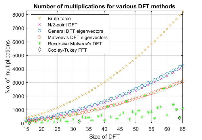
Our analysis has found that the proposed method requires fewer multiplications than when using a single stage Cooley–Tukey algorithm. In fact, if the proposed method is combined with recursive algorithms like the prime factor FFT, the number of multiplications are comparable to the Cooley–Tukey FFT of size $2^k$; $k\in {\mathbb{Z}}^{+}$. Moreover, this method is not restricted by the size of the DFT; unlike the Cooley–Tukey FFT which requires the input length N to be an integer power of 2, or the prime factor FFT which requires N to be a product of coprime numbers.

The methodology is derived in Section 2, which shows the relationship between an input (data) vector, the DFT eigenvectors, and the Fourier transform output. Section 3 deals with the computation of the inverse DFT. The DFT eigenvectors with some favourable properties were derived by Matveev [7] and Section 4 provides a brief description of that technique to find the eigenvectors. In Section 5, a 5-point DFT example is shown using our method developed in this work. Accuracy of the proposed method is discussed in Section 6. In Section 7, the number of real-valued operations required for calculating the DFT using our algorithm is derived.

2. Methodology

A Fourier transform matrix F is diagonalizable and can be decomposed into its Jordan form $F=V\Lambda V^{-1}$ where V is a matrix whose columns are the eigenvectors of F and $\Lambda$ is a purely diagonal matrix containing the eigenvalues of F. Since F is unitary, the eigenvalues in $\Lambda$ have magnitude one and the eigenvector matrix V is also unitary. What may be less well-known is that it is possible find a real and orthonormal set of eigenvectors for F [7]. We use $V^{\mathrm{H}}$ as the complex conjugate transpose of V and $V^{\mathrm{T}}$ as the transpose of V. However, since V is real, $V^{\mathrm{H}}$ is the transpose of V, i.e., $V^{\mathrm{H}}=V^{\mathrm{T}}$. Of course, since V is unitary, $V^{-1}=V^{\mathrm{H}}=V^{\mathrm{T}}$. So, we have the more useful Jordan form

$$F=V\Lambda V^{\mathrm{T}}$$

(3)

Definition 1.

The function $\mathit{diag}\left(·\right)$ converts a vector to a diagonal matrix.

Let $e_i$ be a Euclidean basis vector where the i^th element is 1 and all other elements are zero. Thus, $e_0={\left[\begin{array}{cccc}1& 0& \cdots & 0\end{array}\right]}^{\mathrm{T}}$, $e_1={\left[\begin{array}{ccccc}0& 1& 0& \cdots & 0\end{array}\right]}^{\mathrm{T}}$ and so on. If $a={\left[\begin{array}{cccc}{a}_0& a_1& \cdots & a_{N-1}\end{array}\right]}^{\mathrm{T}}$, $\mathrm{diag}\left(a\right)$ is defined as

$$\begin{array}{cc}\hfill A& =\mathrm{diag}\left(a\right)\hfill \\ \hfill & =\sum _{i=0}^{N-1}{a}_i{e}_i{e}_i^{\mathrm{T}}\hfill \\ \hfill & =\left[\begin{array}{cccc}{a}_0& 0& \cdots & 0\\ 0& a_1& 0& ⋮\\ ⋮& 0& \ddots & 0\\ 0& \cdots & 0& a_{N-1}\end{array}\right]\hfill \end{array}$$

Theorem 1.

If a and b are vectors, and $A=\mathit{diag}\left(a\right)$ and $B=\mathit{diag}\left(b\right)$, then $Ab=Ba$.

Proof. 

Let $a={\left[\begin{array}{cccc}{a}_0& a_1& \cdots & a_{N-1}\end{array}\right]}^{\mathrm{T}}$ and $b={\left[\begin{array}{cccc}{b}_0& b_1& \cdots & b_{N-1}\end{array}\right]}^{\mathrm{T}}$.

$$\begin{array}{cc}\hfill Ab& =\mathrm{diag}\left(a\right)·b\hfill \\ \hfill & =\sum _{i=0}^{N-1}{a}_i{e}_i{e}_i^{\mathrm{T}}b\hfill \\ \hfill & =\sum _{i=0}^{N-1}{a}_i{e}_i{b}_i=\sum _{i=0}^{N-1}{b}_i{e}_i{a}_i\hfill \\ \hfill & =\sum _{i=0}^{N-1}{b}_i{e}_i{e}_i^{\mathrm{T}}a\hfill \\ \hfill & =\mathrm{diag}\left(b\right)·a\hfill \\ \hfill & =Ba\hfill \end{array}$$

This completes the proof. □

If X is the Fourier transform of the vector x and F is the Fourier transform matrix,

$$\begin{array}{cc}\hfill X& =Fx\hfill \\ \hfill & =V\Lambda V^{\mathrm{T}}x\hfill \\ \hfill & =V\Lambda \tilde{x}\hfill \\ \hfill & =V\tilde{X}\lambda \hfill \end{array}$$

(4)

where $\tilde{x}=V^{\mathrm{T}}x$, $\tilde{X}=\mathrm{diag}\left(\tilde{x}\right)$ and $\Lambda =\mathrm{diag}\left(\lambda \right)$ such that $\lambda$ is a column vector containing the eigenvalues of F. Note that $\Lambda \tilde{x}=\tilde{X}\lambda$ from Theorem 1.

In (4), $\lambda$ adds the columns of the matrix product $V\tilde{X}$ in a particular manner defined by the eigenvalues of F. It is well known that there are only four unique eigenvalues for the Fourier transform: $\pm 1$ and $\pm j$, where $j=\sqrt{-1}$ is the imaginary unit [8,9]. Denote the algebraic multiplicity of the DFT eigenvalues as $m_1$, $m_{-1}$, $m_j$ and $m_{-j}$ for the eigenvalues 1, $-1$, j and $-j$, respectively. So, for an N-point DFT, we have $m_1+m_{-1}+m_j+m_{-j}=N$. From [7], these multiplicities are

$$\begin{array}{cccc}\hfill m_1& =⌊\frac{N}{4}⌋+1\hfill & \hfill m_j& =⌊\frac{N-1}{4}⌋\hfill \\ \hfill m_{-1}& =⌊\frac{N+2}{4}⌋\hfill & \hfill m_{-j}& =⌊\frac{N+1}{4}⌋\hfill \end{array}$$

(5)

Without loss of generality, let $\lambda$ in (4) be constructed such that the unique eigenvalues are grouped together as shown in (6). This grouping simplifies our derivation. Note that the eigenvectors in the columns of V will correspond with their respective eigenvalues in the vector $\lambda$.

$$\lambda ={\left[\begin{array}{cccccccccccc}1& \cdots & 1& -1& \cdots & -1& j& \cdots & j& -j& \cdots & -j\end{array}\right]}^{\mathrm{T}}$$

(6)

Let u be an $N\times 2$ matrix as defined in (7) where the first row contains $m_1$ 1’s and $m_{-1}$$-1$’s and the second row contains $m_j$ 1’s and $m_{-j}$$-1$’s.

$$u={\left[\begin{array}{cccccccccccc}1& \cdots & 1& -1& \cdots & -1& 0& & \cdots & & & 0\\ 0& & \cdots & & & 0& 1& \cdots & 1& -1& \cdots & -1\end{array}\right]}^{\mathrm{T}}$$

(7)

From (6) and (7) it is clear that

$$\begin{array}{cc}\hfill \lambda & =u\left[\begin{array}{c}1\\ j\end{array}\right]\hfill \\ \hfill & =uz\hfill \end{array}$$

where $z={\left[\begin{array}{cc}1& j\end{array}\right]}^{\mathrm{T}}$. Now (4) can be rewritten

$$X=V\tilde{X}uz$$

(8)

2.1. Formulations of Equation (8)

If the input vector x is complex such that $x\in {\mathbb{C}}^N$, we can split the real and imaginary components by $x=x_r+j{x}_i$ where $x_r=\mathrm{real}\left(x\right)$ and $x_i=\mathrm{imag}\left(x\right)$. Since $\tilde{X}=\mathrm{diag}\left(V^{\mathrm{T}}x\right)$, we can rewrite (8) by splitting the real and imaginary parts such that ${\tilde{X}}_r=\mathrm{diag}\left(V^{\mathrm{T}}{x}_r\right)$ and ${\tilde{X}}_i=\mathrm{diag}\left(V^{\mathrm{T}}{x}_i\right)$. It is clear that $\tilde{X}={\tilde{X}}_r+j{\tilde{X}}_i$. Now (8) becomes

$$\begin{array}{cc}\hfill X& =V{\tilde{X}}_{r}uz+jV{\tilde{X}}_{i}uz\hfill \end{array}$$

(9)

$$\begin{array}{cc}\hfill & =V{\tilde{X}}_{r}uz+V{\tilde{X}}_{i}u{z}_i\hfill \end{array}$$

(10)

where $z_i=jz={\left[\begin{array}{cc}j& -1\end{array}\right]}^{\mathrm{T}}$. Alternatively, (9) can be implemented by modifying u and keeping z unchanged for the imaginary part. In this case (9) changes to

$$X=V{\tilde{X}}_{r}uz+V{\tilde{X}}_i{u}_{i}z$$

(11)

where $u_i$ is given by (12). The first column of $u_i$ contains $m_j$ -1’s and $m_{-j}$ 1’s and the second column contains $m_1$ 1’s and $m_{-1}$ -1’s. Thus, $u_i$ can be formed by swapping the columns of u followed by negating the first column.

$$u_i={\left[\begin{array}{cccccccccccc}0& & \cdots & & & 0& -1& \cdots & -1& 1& \cdots & 1\\ 1& \cdots & 1& -1& \cdots & -1& 0& & \cdots & & & 0\end{array}\right]}^{\mathrm{T}}$$

(12)

In (10) and (11) both terms on the right-hand-side contain real and imaginary parts. This can be shown by factoring ():

$$\begin{array}{cc}\hfill X& =V\left({\tilde{X}}_{r}u+{\tilde{X}}_i{u}_i\right)z\hfill \\ \hfill & =VWz\hfill \end{array}$$

where the $N\times 2$ matrix $W={\tilde{X}}_{r}u+{\tilde{X}}_i{u}_i$. The first column of W contributes to the real part of the DFT and its second column contributes to the imaginary part of DFT. Therefore, (8) and (9) can be manipulated such that the components of the input that lead to the real and imaginary parts of the DFT are grouped together before computing W. Let ${\tilde{x}}_r=V^{\mathrm{T}}{x}_r$, ${\tilde{x}}_i=V^{\mathrm{T}}{x}_i$ and $m^{\prime }=m_1+m_{-1}$. Create vectors $y_1$ and $y_2$ such that

$$\begin{array}{cc}\hfill y_1& ={\left[\widetilde{x_r}\left(0\right),\cdots ,\widetilde{x_r}\left(m^{\prime }-1\right),\widetilde{x_i}\left(m^{\prime }\right),\cdots ,\widetilde{x_i}\left(N-1\right)\right]}^{\mathrm{T}}\hfill \\ \hfill y_2& ={\left[\widetilde{x_i}\left(0\right),\cdots ,\widetilde{x_i}\left(m^{\prime }-1\right),\widetilde{x_r}\left(m^{\prime }\right),\cdots ,\widetilde{x_r}\left(N-1\right)\right]}^{\mathrm{T}}\hfill \end{array}$$

where the notation ${\tilde{x}}_s\left(k\right)$ represents the k^th element of the vector ${\tilde{x}}_s$ and $s=r,i$. Let $Y^{\prime }=\left[\begin{array}{cc}{Y}_1& Y_2\end{array}\right]$ where $Y_1=\mathrm{diag}\left(y_1\right)$ and $Y_2=\mathrm{diag}\left(y_2\right)$. It is clear that $Y^{\prime }$ is a $N\times 2N$ matrix. Define a $2N\times 2$ matrix $u^{\prime }$ as given in (13). The first column of $u^{\prime }$ is comprised of $m_1$ 1’s, $\left(m_{-1}+m_j\right)$ -1’s followed by $m_{-j}$ 1’s; and the second column consists of $m_1$ 1’s, $m_{-1}$ -1’s, $m_j$ 1’s and $m_{-j}$ -1’s.

$$u^{\prime }={\left[\begin{array}{ccccccccccccccccccccc}1& \cdots & 1& -1& \cdots & -1& 1& \cdots & 1& 0& & & & & \cdots & & & & & & 0\\ 0& & & & \cdots & & & & 0& 1& \cdots & 1& -1& \cdots & -1& 1& \cdots & 1& -1& \cdots & -1\end{array}\right]}^{\mathrm{T}}$$

(13)

With this information, the third formulation of (9) is obtained:

$$X=V{Y}^{\prime }{u}^{\prime }z$$

(14)

Another method to implement (9) is by rearranging the $V^{\mathrm{T}}$ matrix. Define $V^{\prime }$ as

$$V^{\prime }={\left[\begin{array}{cccccc}{v}_0& \cdots & v_{m^{\prime }-1}& 0& \cdots & 0\\ 0& \cdots & 0& v_{m^{\prime }}& \cdots & v_{N-1}\end{array}\right]}^{\mathrm{T}}$$

where the column vector $v_k$ is the k^th eigenvector of F. $V^{\prime }$ is a $N\times 2N$ matrix. Let $x_1=\left[x_r;x_i\right]$ and $x_2=\left[x_i;x_r\right]$, where the semicolon represents the start of a new row. Thus, $x_1$ and $x_2$ are $2N\times 1$ vectors. Let ${\tilde{X}}_1=\mathrm{diag}\left(V^{\prime }{x}_1\right)$, ${\tilde{X}}_2=\mathrm{diag}\left(V^{\prime }{x}_2\right)$ and $X^{\prime }=\left[\begin{array}{cc}{\tilde{X}}_1& {\tilde{X}}_2\end{array}\right]$, where $X^{\prime }$ has size $N\times 2N$. Now (9) can be rephrased as

$$X=V{X}^{\prime }{u}^{\prime }z$$

(15)

Here we have presented four different formulations of (9) via (10), (11), (14) and (15). Each of these formulations affects a different factor in (8). In these equations the only complex component is contained in either z or $z_i$. The vector z or $z_i$ is not necessary for the computational algorithm, only for theoretical completeness. Thus, all the multiplications and additions are real-valued. Therefore, we say that this method of computing the DFT is natively-real valued because it can be computed using operations whose operands are all real numbers (in $\mathbb{R}$).

2.2. Real Inputs

If x is real such that $x\in {\mathbb{R}}^N$, the four different forms given in (10), (11), (14) and (15) simplify to

$$X=V{\tilde{X}}_{r}uz$$

which is exactly (8) since $\tilde{X}={\tilde{X}}_r$. This is very straightforward in (10) and (11). In both these cases the second term is 0 since $x_i=0$. For the other terms, the matrix product $Y^{\prime }{u}^{\prime }$ or $X^{\prime }{u}^{\prime }$ simplifies to ${\tilde{X}}_{r}u$. Since x is real, the product $V\tilde{X}u$ in (8) results in an $N\times 2$ matrix whose first column contains the real component of the DFT X, and the second column is the imaginary component of X. As mentioned before, the vector z is not necessary for the computational algorithm; z just clarifies that the first column is real and the second column is imaginary.

2.3. A Filter Bank Model/Interpretation

Since $\tilde{X}=\mathrm{diag}\left(V^{\mathrm{T}}x\right)$, the diagonal entries of $\tilde{X}$ are formed by the inner product of the DFT eigenvectors and the input x. Let $V=\left[\begin{array}{cccc}{v}_0& v_1& \cdots & v_{N-1}\end{array}\right]$ where the column vector $v_k$ is a DFT eigenvector. Thus

$$\tilde{X}=\left[\begin{array}{cccc}〈v_0,x〉& 0& \cdots & 0\\ 0& 〈v_1,x〉& 0& ⋮\\ ⋮& 0& \ddots & 0\\ 0& \cdots & 0& 〈v_{N-1},x〉\end{array}\right]$$

(16)

where the notation $〈a,b〉$ represents the inner (dot) product of two vectors a and b. We use this to develop a filter bank description for the linear algebra in the above discussion. Specifically, we define the time reversed vector $v_0(-n)$ of $v_0$. Now, filter the sequence x through the FIR filter $v_0(-n)$ to produce the $N+N-1=2N-1$ length output sequence $x_0^{filt}$. Down-sample this output $x_0^{filt}$ by N (i.e., selecting the middle term) yields the dot product $〈v_0,x〉$, i.e., $〈v_0,x〉=x_0^{filt}\left(N-1\right)$, where $x_0^{filt}\left(N-1\right)$ is the N^th element of $x_0^{filt}$. A similar procedure is applied to the other eigenvectors.

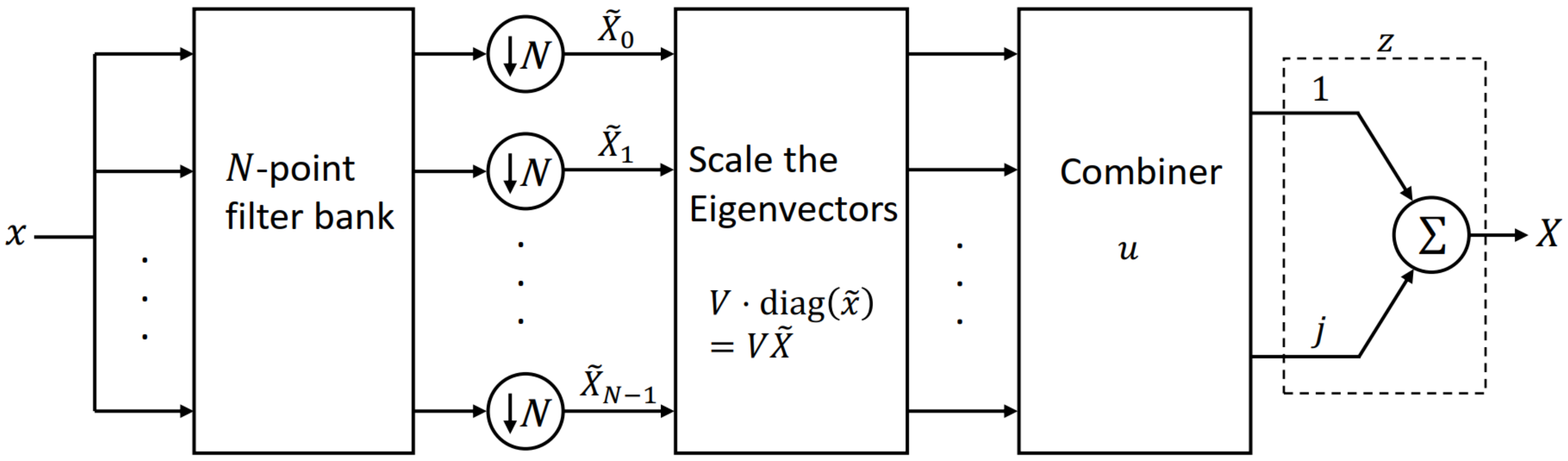
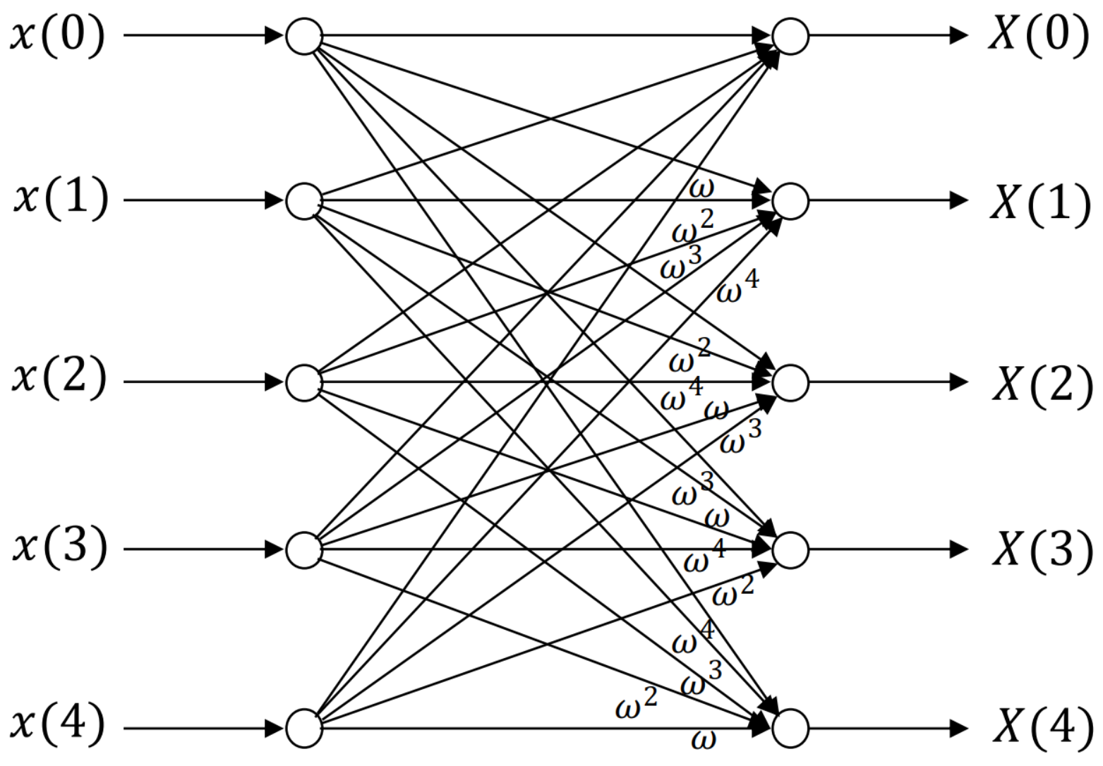
Now consider the matrix product $V\tilde{X}$. Each diagonal entry of $\tilde{X}$ scales the corresponding column of V, i.e., each eigenvector is scaled by the corresponding filter output. These scaled eigenvectors are then added or subtracted in the specific manner defined by u to give the real and imaginary components of the DFT result. This is why we call u the “combiner”. The combiner adds and subtracts the real parts (from the $\pm 1$ elements of u) and the imaginary components (from the $\pm j$ of u). The vector z is only provided for theoretical completeness so that we can combine the real and imaginary components for the DFT X. These steps are summarized in Figure 1.

3. Inverse DFT

The IDFT (inverse DFT) computation follows a similar development. The IDFT has the same unique eigenvalues as the DFT, only they differ in the eigenvalue multiplicity for eigenvalues j and $-j$. Due to the conjugation difference in the DFT and the IDFT, the multiplicities of these eigenvalues are exchanged. Consequently, the eigenvalue multiplicities of the IDFT are

$$\begin{array}{cccc}\hfill m_1& =⌊\frac{N}{4}⌋+1\hfill & \hfill m_j& =⌊\frac{N+1}{4}⌋\hfill \\ \hfill m_{-1}& =⌊\frac{N+2}{4}⌋\hfill & \hfill m_{-j}& =⌊\frac{N-1}{4}⌋\hfill \end{array}$$

(17)

Similarly, the eigenvectors are unchanged from the DFT for the eigenvalues 1 and $-1$, but they are exchanged for eigenvalues j and $-j$. Thus, the eigenvector matrix for the IDFT $V_{\mathrm{IDFT}}$ can be obtained directly from the DFT eigenvector matrix V.

Using $V_{\mathrm{IDFT}}$, the steps described in Section 2 can be used to compute the IDFT. The block diagram of the IDFT follows directly from these definitions used to replace the DFT computations used to derive Figure 1. As in the case for the DFT, symmetries found in the input sequence can be used to improve the computational efficiency. Moreover, if the input or the output sequence is known to be real valued, the computational efficiency can be improved further. If the input to the IDFT is real, the procedure is similar to the DFT with real inputs.

However, if the output of the IDFT is known to be real, the input will be complex and will have some symmetries which can be exploited to improve computational performance. Let $x=\mathrm{IDFT}\left(X\right)$, where $X=X_r+X_i$ such that $X_r=\mathrm{real}\left(X\right)$ and $X_i=\mathrm{imag}\left(X\right)$. If x is real, $X_r$ will be even symmetric and $X_i$ will be odd symmetric (ch. 5 [10]). 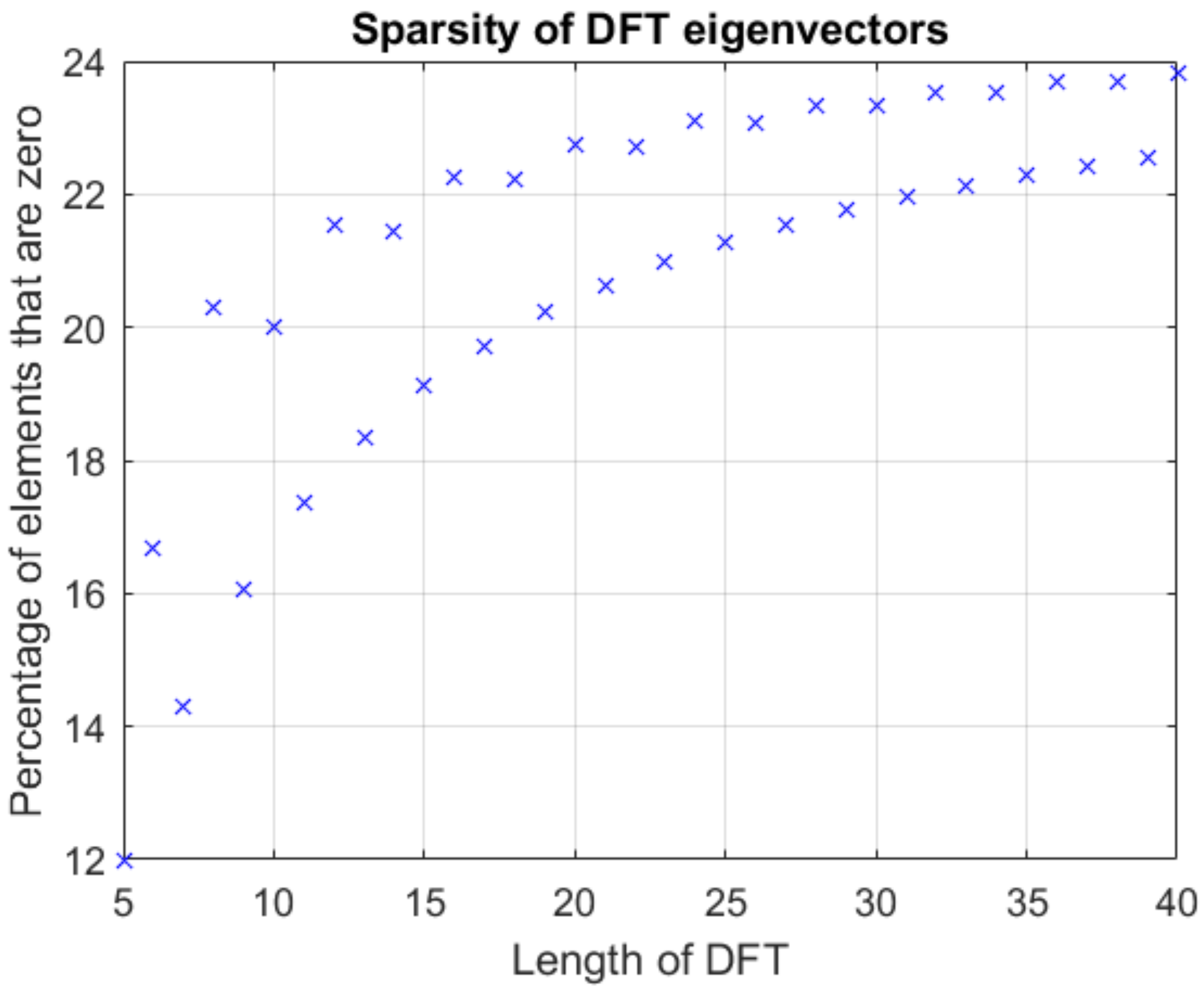It is also known that the DFT eigenvectors are either even symmetric (for eigenvalues $\pm 1$) or odd symmetric (for eigenvalues $\pm j$) [8]. These eigenvector symmetries are further explored in Section 7. Let $v_{ev}$ represent an even symmetric eigenvector for eigenvalues $\pm 1$ and $v_{od}$ denote an odd symmetric eigenvector for eigenvalues $\pm j$. It is well understood that the product (Hadamard product) of two even sequences or two odd sequences will be even, and the product of an even and an odd sequence will be odd. We also know that the sum of the elements of an even sequence will be twice the sum of the first half of the sequence and the sum of the elements of an odd sequence will be zero. Combining this information for the calculation of the inner products for ${\tilde{X}}_r$ and ${\tilde{X}}_i$ in (10), we get $〈X_r,v_{od}〉=〈X_i,v_{ev}〉=0$ and $〈X_r,v_{ev}〉$, $〈X_i,v_{od}〉$ require approximately $N/2$ multiplications each. Therefore, the last $N-m^{\prime }$ diagonal entries of ${\tilde{X}}_r$ and the first $m^{\prime }$ diagonal elements of ${\tilde{X}}_i$ will be 0 where $m^{\prime }=m_1+m_{-1}$. Thus, both the terms of (10) will be purely real. Similarly, for (14), $Y^{\prime }=Y$ since $Y_2=0$ again leading to a reduction in the number of operations. Comparable patterns also exist for (11) and (15).

4. Computing Orthonormal Eigenvectors of the DFT

Several methods exist to find the real and orthonormal eigenvectors of the DFT. The method described by McClellan and Parks [8] only yields real eigenvectors. These eigenvectors can be orthonormalized using the Gram–Schmidt process. Matveev [7] uses DFT projection matrices and their Grammian determinants to find the orthonormal eigenvectors directly. Alternatively, the DFT projection matrices [7,9] can be used in conjunction with the Gram–Schmidt process to obtain orthonormal eigenvectors. Our method performs equally well regardless of the method used to find the orthonormal real-valued eigenvectors.

4.1. Matveev Method

The first step in the Matveev method is to compute the four projection matrices of the DFT corresponding to each unique eigenvalue. If $P_e$ is a projection matrix corresponding to an eigenvalue e, F is the Fourier transform matrix and I is the identity matrix,

$$\begin{array}{cc}\hfill P_1& =\frac{1}{4}\left(F^3+F^2+F+I\right)\hfill \\ \hfill P_{-1}& =\frac{1}{4}\left(-F^3+F^2-F+I\right)\hfill \\ \hfill P_j& =\frac{1}{4}\left(j{F}^3-F^2-jF+I\right)\hfill \\ \hfill P_{-j}& =\frac{1}{4}\left(-j{F}^3-F^2+jF+I\right)\hfill \end{array}$$

(18)

The rank of each of these matrices is tied to their corresponding eigenvalue multiplicity. Thus, the matrix $P_e$ will be rank $m_e$. Therefore, to compute the orthogonal eigenvectors only the first $m_1$ and $m_{-1}$ columns of $P_1$ and $P_{-1}$ are considered; the first column of $P_j$ and $P_{-j}$ are ignored and only the next $m_j$ and $m_{-j}$ columns are considered. The first columns of $P_j$ and $P_{-j}$ are ignored because they are zeros. The kept columns form independent eigenvectors of F corresponding to each respective eigenvalue.

Let the elements of the matrices in (18) be represented as $P_e\left(m,n\right)$. For example, if the indexing starts from 0, the element in the second row and first column of $P_{-1}$ will be $P_{-1}\left(1,0\right)$. Therefore, the last element will be $P_{-1}\left(N-1,N-1\right)$. Let the columns of these matrices be represented as $p_{e,k}$, where $p_{e,k}$ is the k^th column vector of $P_e$. For example, the third column vector of $P_j$ will be $p_{j,2}$, again assuming the indexing starts from 0. Note that these projection matrices are symmetric. Therefore, the k^th column will also be the k^th row.

The orthogonal eigenvectors are given by the determinants of the following matrices. For eigenvalues $e=\left\{1,-1\right\}$,

$${\beta }_{e,0}=p_{e,0}$$

$${\beta }_{e,1}=\left|\begin{array}{cc}{P}_e\left(0,0\right)& p_{e,0}\\ P_e\left(1,0\right)& p_{e,1}\end{array}\right|$$

$${\beta }_{e,k}=\left|\begin{array}{ccccc}{P}_e\left(0,0\right)& P_e\left(0,1\right)& \cdots & P_e\left(0,k-1\right)& p_{e,0}\\ P_e\left(1,0\right)& P_e\left(1,1\right)& & P_e\left(1,k-1\right)& p_{e,1}\\ ⋮& & \ddots & ⋮& ⋮\\ P_e\left(k,0\right)& P_e\left(k,1\right)& \cdots & P_e\left(k,k-1\right)& p_{e,k}\end{array}\right|$$

where ${\beta }_{e,k}$ form a set of orthogonal eigenvectors corresponding to eigenvalues $e=\left\{1,-1\right\}$ and $1\le k\le m_e-1$. ${\beta }_{e,1}$ gives the eigenvector when $k=1$. Because these matrices contain scalars $P_e\left(m,n\right)$ and vectors $p_{e,k}$, the determinant can be computed by expanding along the last column and multiplying these vectors by their corresponding cofactors. Similarly, for eigenvalues $e=\left\{j,-j\right\}$,

$${\beta }_{e,0}=p_{e,1}$$

$${\beta }_{e,1}=\left|\begin{array}{cc}{P}_e\left(1,1\right)& p_{e,1}\\ P_e\left(2,1\right)& p_{e,2}\end{array}\right|$$

$${\beta }_{e,k}=\left|\begin{array}{ccccc}{P}_e\left(1,1\right)& P_e\left(1,2\right)& \cdots & P_e\left(1,k\right)& p_{e,1}\\ P_e\left(2,1\right)& P_e\left(2,2\right)& & P_e\left(2,k\right)& p_{e,2}\\ ⋮& & \ddots & ⋮& ⋮\\ P_e\left(k+1,0\right)& P_e\left(k+1,2\right)& \cdots & P_e\left(k+1,k\right)& p_{e,k+1}\end{array}\right|$$

where ${\beta }_{e,k}$ is the general equation. Here also $1\le k\le m_e-1$. Note that if $e=\left\{j,-j\right\}$, for the projection matrix $P_e$ the elements of the first row $P_e\left(0,k\right)$, first column $P_e\left(k,0\right)$ and the first column vector $p_{e,0}$ are not considered since they are zeros. The determinant for these matrices can be computed using the method explained in the previous paragraph for the real eigenvalues.

In both cases, the resulting vectors ${\beta }_{e,k}$ are orthogonal but not unit length. After normalization, the columns of the eigenvector matrix matrix V are

$$v_{e,k}=\frac{{\beta }_{e,k}}{∥{\beta }_{e,k}∥}$$

Although (18) contains powers of the Fourier transform matrix, it is not necessary to numerically calculate those powers. Using the properties of the DFT, $F^3=F^{\mathrm{H}}$, where $F^{\mathrm{H}}$ represents the complex conjugate transpose of F. $F^2$ will be a real matrix such that $F^2=\left[\begin{array}{cccccc}{I}_0& I_{N-1}& I_{N-2}& \cdots & I_2& I_1\end{array}\right]$, where $I_k$ is the k^th column of the identity matrix I assuming the indexing starts from 0.

4.2. Gram–Schmidt Orthonormalization

Numerically similar orthonormal eigenvectors can be found from (18) via the Gram–Schmidt orthonormalization process. As discussed before, the matrices $P_e$ are not full rank. Therefore, we only consider the first $m_1$ and $m_{-1}$ columns of $P_1$ and $P_{-1}$; ignore the first column of $P_j$ and $P_{-j}$ and consider the next $m_j$ and $m_{-j}$ columns. In our observation, using Gram–Schmidt orthonormalization on the DFT projection matrices gives the fastest and most numerically accurate results when run on MATLAB©. Accuracy tests and their results are discussed in Section 6. We observed that the eigenvectors obtained using the Matveev method is somewhat sparse. That same sparse structure is retained by the Gram–Schmidt orthonormalization of the DFT projection matrices as well as the Gram–Schmidt orthonormalization of McClellan and Parks eigenvectors.

4.3. Structure of Eigenvectors

The eigenvectors obtained using McClellan and Parks method are collinear to the eigenvectors from the DFT projection matrices and they differ only in magnitude. As discussed before, orthonormalizing these eigenvectors make them slightly sparse. These orthonormal eigenvectors have the following structure:

$$V_{\pm 1}=\left[\begin{array}{cccc}{a}_0& 0& 0& 0\\ a_1& b_1& 0& 0& \cdots \\ a_1& b_2& c_2& 0\\ a_1& b_3& c_3& d_4\\ ⋮& ⋮& ⋮& ⋮\\ a_1& b_3& c_3& d_4\\ a_1& b_2& c_2& 0& \cdots \\ a_1& b_1& 0& 0\end{array}\right]V_{\pm j}=\left[\begin{array}{ccc}0& 0& 0\\ b_1& 0& 0& \cdots \\ b_2& c_2& 0\\ b_3& c_3& d_4\\ ⋮& ⋮& ⋮\\ -b_3& -c_3& -d_4\\ -b_2& -c_2& 0& \cdots \\ -b_1& 0& 0\end{array}\right]$$

where the matrix $V_{\pm 1}$ represents the set of orthonormal eigenvectors corresponding to eigenvalues $\pm 1$ and $V_{\pm j}$ represent the orthonormal eigenvectors corresponding to eigenvalues $\pm j$. The columns of these matrices represent the eigenvectors. The vectors in $V_{\pm 1}$ is even symmetric and the vectors in $V_{\pm j}$ is odd symmetric. Additionally, if the size of DFT N is an even value, the $\left(\frac{N}{2}+1\right)$^th row of $V_{\pm j}$ will be 0 to retain the odd symmetry. The sparsity of the eigenvectors are shown in Figure 2. From this plot, it is clear that the orthonormal DFT eigenvectors are somewhat sparse. This sparse nature can be exploited to reduce the number of operations required while computing the DFT as discussed in Section 7.

The orthonormal eigenvectors of an 8-point DFT are given below to highlight the sparsity. The eigenvectors are the columns of the matrix $V_8$. The eigenvalue multiplicities of an 8-point DFT are 3, 2, 1, 2 for eigenvalues 1, $-1$, j, $-j$, respectively. Therefore, the first three columns of $V_8$ are the eigenvectors corresponding to the eigenvalue 1, the next two columns are for eigenvalue $-1$, the column after that is for eigenvalue j and the last two columns correspond to eigenvalue $-j$.

$$V_8=\left[\begin{array}{cccccccc}0.823& 0& 0& 0.569& 0& 0& 0& 0\\ 0.215& 0.573& 0& -0.311& 0.168& 0.354& 0.612& 0\\ 0.215& -0.081& 0.143& -0.311& -0.575& -0.500& 0.289& 0.408\\ 0.215& -0.299& -0.490& -0.311& 0.168& -0.354& 0.204& -0.577\\ 0.215& -0.389& 0.692& -0.311& 0.476& 0& 0& 0\\ 0.215& -0.3& -0.490& -0.311& 0.168& 0.354& -0.204& 0.577\\ 0.215& -0.081& 0.143& -0.311& -0.575& 0.500& -0.289& -0.408\\ 0.215& 0.573& 0& -0.311& 0.168& -0.354& -0.612& 0\end{array}\right]$$

5. An Example with 5-Point DFT

5.1. Forward DFT

The eigenvalue multiplicity for a 5-point DFT is $m=\left\{2,1,1,1\right\}$ for the unique eigenvalues $\left\{1,-1,j,-j\right\}$, or we can just say that the eigenvalues are $\left\{1,1,-1,j,-j\right\}$. The orthonormal eigenvectors from the Matveev method as described in Section 4 computed in MATLAB© to double precision are

$$V=\left[\begin{array}{ccccc}0.851& 0& 0.526& 0& 0\\ 0.263& 0.5& -0.425& 0.193& 0.68\\ 0.263& -0.5& -0.425& -0.68& 0.193\\ 0.263& -0.5& -0.425& 0.68& -0.193\\ 0.263& 0.5& -0.425& -0.193& -0.68\end{array}\right]$$

(19)

Now, suppose that the input signal is $x={\left[\begin{array}{ccccc}-2& 0& 3& 1& 1\end{array}\right]}^{\mathrm{T}}$. Then

$$\tilde{x}=V^{\mathrm{T}}x=\left[\begin{array}{c}-0.387\\ -1.5\\ -3.178\\ -1.554\\ -0.294\end{array}\right]$$

If $\tilde{X}=\mathrm{diag}\left(\tilde{x}\right)$ and $\widehat{X}=V\tilde{X}$, then

$$\begin{array}{cc}\hfill \widehat{X}& =\left[\begin{array}{ccccc}-0.329& 0& -1.671& 0& 0\\ -0.102& -0.75& 1.352& -0.3& -0.2\\ -0.102& 0.75& 1.352& 1.057& -0.057\\ -0.102& 0.75& 1.352& -1.057& 0.057\\ -0.102& -0.75& 1.352& 0.3& 0.2\end{array}\right]\hfill \\ \hfill & =\left[\begin{array}{ccccc}{\widehat{x}}_0& {\widehat{x}}_1& {\widehat{x}}_2& {\widehat{x}}_3& {\widehat{x}}_4\end{array}\right]\hfill \end{array}$$

From the eigenvalue multiplicity we know that the DFT X of x is

$$X={\widehat{x}}_0+{\widehat{x}}_1-{\widehat{x}}_2+j\left({\widehat{x}}_3-{\widehat{x}}_4\right)$$

$$\Rightarrow X=\left[\begin{array}{c}1.342\\ -2.203-0.1j\\ -0.703+1.113j\\ -0.703-1.113j\\ -2.203+0.1j\end{array}\right]$$

(20)

5.2. Inverse DFT

As mentioned in Section 3, the eigenvectors for the inverse operation can be constructed from (19) by interchanging the eigenvectors corresponding to the eigenvalues j and $-j$. Thus, the eigenvector matrix for the 5-point IDFT is

$$V_{\mathrm{IDFT}}=\left[\begin{array}{ccccc}0.851& 0& 0.526& 0& 0\\ 0.263& 0.5& -0.425& 0.68& 0.193\\ 0.263& -0.5& -0.425& 0.193& -0.68\\ 0.263& -0.5& -0.425& -0.193& 0.68\\ 0.263& 0.5& -0.425& -0.68& -0.193\end{array}\right]$$

If y is taken from (20), $\tilde{y}=V_{\mathrm{IDFT}}y$.

$$\tilde{y}=\left[\begin{array}{c}-0.387\\ -1.5\\ 3.178\\ 0.294j\\ -1.554j\end{array}\right]$$

If $\widehat{Y}=V_{\mathrm{IDFT}}·\mathrm{diag}\left(\tilde{y}\right)$,

$$\widehat{Y}=\left[\begin{array}{ccccc}-0.329& 0& 1.671& 0& 0\\ -0.102& -0.75& -1.352& 0.12j& -0.3j\\ -0.102& 0.75& -1.352& 0.057j& 1.057j\\ -0.102& 0.75& -1.352& -0.057j& -1.057j\\ -0.102& -0.75& -1.352& -0.12j& 0.3j\end{array}\right]$$

The eigenvalue multiplicity for the 5-point IDFT is $\left\{2,1,1,1\right\}$ for eigenvalues $\{1,-1,j,$$-j\}$. Summing the columns of $\widehat{Y}$ using the information from the eigenvalue multiplicity, we get

$$x={\widehat{y}}_0+{\widehat{y}}_1-{\widehat{y}}_2+j\left({\widehat{y}}_3-{\widehat{y}}_4\right)$$

where ${\widehat{y}}_k$ is the k^th column of $\widehat{Y}$. Thus,

$$x=\left[\begin{array}{c}-2\\ 0\\ 3\\ 1\\ 1\end{array}\right]$$

This is the signal that we started with while computing the forward DFT.

6. Accuracy and Performance of DFT Eigenvector Computation

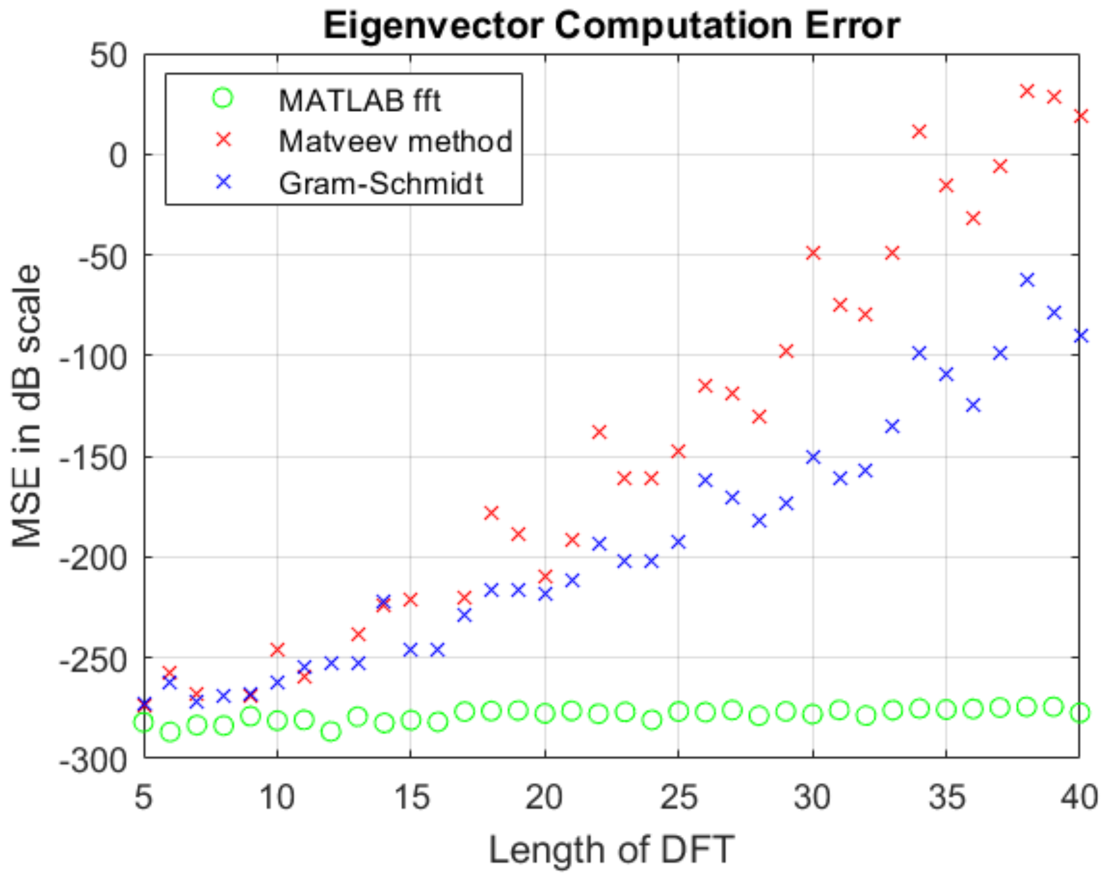
The two different methods used to calculate the orthonormal eigenvectors yield different computational accuracies. These differences arise due to the limitations imposed by the finite-precision data types that are used in real-world machines, and the varying methods used to produce the sparse eigenvectors. We compare the DFTs created using the Matveev method and the Gram–Schmidt orthonormalization of DFT projection matrices. All tests are run using the double-precision floating point data type on MATLAB version 2020b on a machine with Intel(R) Core(TM) i7-6700HQ @ 2.60GHz 4 core CPU, 8 GB RAM and Windows 10 operating system.

Figure 3 indicates the computational error due to imprecise DFT eigenvectors. Suppose x is a vector in ${\mathbb{R}}^n$ and $y=\mathrm{IDFT}\left(\mathrm{DFT}\left(x\right)\right)$. The figure shows the mean squared error (MSE) of $x-y$ in decibels. The DFT and IDFT is calculated using Matveev eigenvectors, Gram–Schmidt orthonormalization of DFT projection matrices, and using the MATLAB fft() and ifft() functions. The MSE is calculated via (21), (22) and (23) where n is the length of the vectors x and y and the operator $∥x∥$ represents the 2-norm of x. The error shown in Figure 3 is caused by the limitation imposed by the machine that was used to compute the eigenvectors. More powerful machines can be used to pre-compute the eigenvectors to a high enough precision such that this error can be eliminated.

$$\mathrm{MSE}=10{log}_{10}\left(\mu \right)$$

(21)

where

$$\mu =\frac{1}{1000}\sum _{i=1}^{1000}{\sigma }_i$$

(22)

and

$$\sigma =\frac{{∥x-y∥}^2}{n}$$

(23)

Here ${\sigma }_i$ represents $i^{th}$ sample out of 1000 samples as explained below.

For each n-point DFT, 1000 vectors are randomly generated such that each element of a vector x is an integer that lies between −128 and 127. These limits are chosen because we can represent the pixels of an 8-bit image after centering the pixel values to 0. For each vector x, the corresponding y and $\sigma$ are computed. Equation (22) gives the average $\sigma$ value of the 1000 samples and (21) gives the average MSE in dB. The plot in Figure 3 shows the error after computing the forward and inverse DFT. Therefore, the error while finding the DFT in one direction will be slightly lower than what is shown and will depend on the size of DFT. Clearly, the computational performance of the eigenvector methods suffers a bit, especially as the length of the DFT increases. The differences are not significant for lengths up to 20, and the method’s complexity analysis in Section 7 will show why these approaches are attractive.

The time required to calculate the eigenvectors from the DFT projection matrices and orthonormalizing them with Matveev method and Gram–Schmidt process is summarized in

Table 1. Computation time in seconds for 10,000 runs.

Length of DFT:	10	20	30	40
Matveev	0.919	3.354	6.460	10.452
Gram–Schmidt	0.684	1.303	2.269	3.694

. In this table, the time is calculated for 10,000 executions of each of the methods and is shown in units of seconds. This is consistent with our rudimentary analysis of the computational complexity of each of the methods: $O\left(n^3\right)$ for Gram–Schmidt and $O\left(n^5\right)$ for Matveev method (assuming the required matrix determinant is computed in $O\left(n^3\right)$ complexity). This discrepancy arises from the need for calculating the determinant of the $\beta$ matrix in the Matveev method, whereas the vector dot product can be calculated in $O\left(n\right)$ time for the Gram–Schmidt process.

7. Number of Operations

7.1. Using Generalized Eigenvectors

At first glance while observing (8), computing $\tilde{X}$ seems to need N multiplications and $N-1$ additions assuming that $x\in {\mathbb{R}}^N$. However, as briefly discussed in Section 3, it is known that all the eigenvectors of the DFT are either even or odd symmetric sequences [8]. Eigenvectors corresponding to eigenvalues 1 or $-1$ will be even symmetric, and eigenvectors corresponding to eigenvalues j or $-j$ will be odd symmetric. Using this property, if an eigenvector $v_k$ is even symmetric, $〈v_k,x〉$ in (16) can be computed using $⌊N/2⌋+1$ real multiplications and $N-1$ real additions. If $v_k$ is an odd symmetric eigenvector, the inner product requires $⌊N/2⌋$ real multiplications and $N-2$ real additions because the first element of $v_k$ will be 0 in this case. For example, consider an even eigenvector of a 5-point DFT $v_{ev}={\left[\begin{array}{ccccc}{a}_0& a_1& a_2& a_2& a_1\end{array}\right]}^{\mathrm{T}}$. For an input vector $x={\left[\begin{array}{ccccc}{x}_0& x_1& x_2& x_3& x_4\end{array}\right]}^{\mathrm{T}}$,

$$\begin{array}{cc}\hfill 〈v_{ev},x〉& =a_0{x}_0+a_1{x}_1+a_2{x}_2+a_2{x}_3+a_1{x}_4\hfill \\ \hfill & =a_0{x}_0+a_1(x_1+x_4)+a_2(x_2+x_3)\hfill \end{array}$$

(24)

The first line requires five multiplications, and the second line requires three multiplications. The number of additions in both cases is 5. Now consider an odd eigenvector of a 5-point DFT $v_{od}={\left[\begin{array}{ccccc}0& b_1& b_2& -b_2& -b_1\end{array}\right]}^{\mathrm{T}}$.

$$\begin{array}{cc}\hfill 〈v_{od},x〉& =0+b_1{x}_1+b_2{x}_2-b_2{x}_3-b_1{x}_4\hfill \\ \hfill & =b_1(x_1-x_4)+b_2(x_2-x_3)\hfill \end{array}$$

(25)

Here using the symmetry, there are two multiplications and three additions. Similar relationships can be found for even length sequences.

We know that the number of even or odd eigenvectors depends on the eigenvalue multiplicity (which in turn depends on N). The number of even eigenvectors is $m_1+m_{-1}$ and the number of odd eigenvectors is $m_j+m_{-j}$. Thus, for computing $\tilde{X}$ in (16) the total number of multiplications ${\Xi }_{\tilde{X}}\left(N\right)$ and number of additions ${\mathrm{\Phi }}_{\tilde{X}}\left(N\right)$ required are

$$\begin{array}{cc}\hfill {\Xi }_{\tilde{X}}\left(N\right)& =\left(⌊\frac{N}{2}⌋+1\right)\left(m_1+m_{-1}\right)+⌊\frac{N}{2}⌋\left(m_j+m_{-j}\right)\hfill \end{array}$$

$${\mathrm{\Phi }}_{\tilde{X}}\left(N\right)=\left(N-1\right)\left(m_1+m_{-1}\right)+\left(N-2\right)\left(m_j+m_{-j}\right)$$

For large values of N the eigenvalue multiplicities can be approximated to be equal to each other (which in turn approximately equals $N/4$). Thus, $m_1\approx m_{-1}\approx m_j\approx m_{-j}\approx N/4$. Therefore for large N,

$${\Xi }_{\tilde{X}}\left(N\right)\approx \frac{N^2}{2}$$

$$\begin{array}{cc}\hfill {\mathrm{\Phi }}_{\tilde{X}}\left(N\right)& \approx \frac{N}{2}\left(2N-3\right)\approx N^2\hfill \end{array}$$

While multiplying the eigenvector matrix with $\tilde{X}$ in (4) and (8) the eigenvector symmetry can be utilized again. Let $W=V\tilde{X}$. Let the number of multiplications required for computing $V\tilde{X}$ be ${\Xi }_W\left(N\right)$ and the number of additions be ${\mathrm{\Phi }}_W\left(N\right)$. So, ${\Xi }_W\left(N\right)={\Xi }_{\tilde{X}}\left(N\right)$ due to the symmetry of the eigenvectors in V. As noted before, the operation $V\tilde{X}$ just changes the magnitude of each eigenvector. Therefore, the columns of W retain the even or odd symmetries of the eigenvectors. From (8) we know that the columns of W are added in a specific pattern to determine the DFT. Thus, the result of this sum will also be even or odd symmetric. Therefore, while adding the columns of W, only the top half of the elements need to be computed (and the “middle” value). Thus, the number of additions required is

$${\mathrm{\Phi }}_W\left(N\right)=\left(⌊\frac{N}{2}⌋+1\right)\left(m_1+m_{-1}\right)+⌊\frac{N}{2}⌋\left(m_j+m_{-j}\right)$$

When N is large

$${\mathrm{\Phi }}_W\left(N\right)\approx \frac{N^2}{2}$$

The total number of multiplications and additions required is

$$\begin{array}{cc}\hfill \Xi \left(N\right)& ={\Xi }_{\tilde{X}}\left(N\right)+{\Xi }_W\left(N\right)\hfill \\ \hfill & =2\left[\left(⌊\frac{N}{2}⌋+1\right)\left(m_1+m_{-1}\right)+⌊\frac{N}{2}⌋\left(m_j+m_{-j}\right)\right]\hfill \end{array}$$

(26)

$$\begin{array}{cc}\hfill \mathrm{\Phi }\left(N\right)& ={\mathrm{\Phi }}_{\tilde{X}}\left(N\right)+{\mathrm{\Phi }}_W\left(N\right)\hfill \\ \hfill & =\left(N+⌊\frac{N}{2}⌋\right)\left(m_1+m_{-1}\right)\hfill \\ \hfill & +\left(N+⌊\frac{N}{2}⌋-2\right)\left(m_j+m_{-j}\right)\hfill \end{array}$$

(27)

For large values of N, these are approximated as

$$\Xi \left(N\right)\approx N^2$$

(28)

$$\mathrm{\Phi }\left(N\right)\approx \frac{3}{2}{N}^2$$

(29)

7.2. Using the Sparsity of the Eigenvectors

Further gains can be obtained if the sparse eigenvectors obtained from the Matveev method (Section 4) are used to find the orthonormal DFT eigenvectors. The Matveev DFT eigenvectors contain a few patterns which can be exploited as explained below.

7.2.1. Zeros in Many Eigenvectors

Elements in the starting and ending indices of many of these eigenvectors are zeros. More of these elements are zeros for larger values of N. For example, if the first even eigenvector calculated using the Matveev method is $v_{ev}={\left[\begin{array}{ccccccc}{a}_0& a_1& a_2& a_3& a_3& a_2& a_1\end{array}\right]}^{\mathrm{T}}$, the second eigenvector will have $a_0=0$, the third will have $a_0=a_1=0$ and so on. A similar pattern also exists for the odd eigenvectors.

7.2.2. Repeating Elements

The first eigenvectors corresponding to the eigenvalues $\pm 1$ are made of only two scalar elements each, i.e., they are of the form $v={\left[\begin{array}{ccccc}{a}_0& a_1& a_1& a_1& a_1\end{array}\right]}^{\mathrm{T}}$.

7.2.3. Zeros in Eigenvectors of Even Length

The middle element of the eigenvectors corresponding to the eigenvalues $\pm j$ are zero, if the eigenvectors are of even length. Thus, if N is the length of the eigenvector, then the ${\left(N/2+1\right)}^{\mathrm{th}}$ element will be 0 if N is even. For example, $v=\left[\begin{array}{cccccc}0& a_1& a_2& 0& -a_2& -a_1\end{array}\right]$ is a possible configuration of such an eigenvector. Note that in this example, the first element is 0 because the vector is odd symmetric.

Using this new information the number of multiplications ${\Xi }_{\tilde{X}}\left(N\right)$ and additions ${\mathrm{\Phi }}_{\tilde{X}}\left(N\right)$ required for calculating $\tilde{X}$ is

$$\begin{array}{cc}\hfill {\Xi }_{\tilde{X}}\left(N\right)& =\left(m_1-1\right)\left(⌊\frac{N}{2}⌋-\frac{m_1-2}{2}\right)+2\hfill \\ \hfill & +\left(m_{-1}-1\right)\left(⌊\frac{N}{2}⌋-\frac{m_{-1}-2}{2}\right)+2\hfill \\ \hfill & +m_j\left(⌊\frac{N-1}{2}⌋-\frac{m_j-1}{2}\right)\hfill \\ \hfill & +m_{-j}\left(⌊\frac{N-1}{2}⌋-\frac{m_{-j}-1}{2}\right)\hfill \end{array}$$

(30)

$$\begin{array}{cc}\hfill {\mathrm{\Phi }}_{\tilde{X}}\left(N\right)& =m_{1}N-m_1\left(m_1-1\right)-1\hfill \\ \hfill & +m_{-1}N-m_{-1}\left(m_{-1}-1\right)-1\hfill \\ \hfill & +2m_j⌊\frac{N-1}{2}⌋-m_j^2\hfill \\ \hfill & +2m_{-j}⌊\frac{N-1}{2}⌋-m_{-j}^2\hfill \end{array}$$

(31)

For the matrix multiplication $W=V\tilde{X}$, the number of scalar multiplications required is ${\Xi }_W\left(N\right)={\Xi }_{\tilde{X}}\left(N\right)$. The number of scalar additions required for adding the columns vectors of W is

$$\begin{array}{cc}\hfill {\mathrm{\Phi }}_W\left(N\right)& =m_{-1}^2+\left(m_1+m_{-1}-1\right)\left(⌊\frac{N}{2}⌋+1-m_{-1}\right)\hfill \\ \hfill & +m_j^2+\left(m_j+m_{-j}-1\right)\left(⌊\frac{N-1}{2}⌋-m_j\right)\hfill \end{array}$$

(32)

From (30)–(32) the total number of multiplications and additions required using Matveev method is

$$\begin{array}{cc}\hfill \Xi \left(N\right)& ={\Xi }_{\tilde{X}}\left(N\right)+{\Xi }_W\left(N\right)\hfill \\ \hfill & =2{\Xi }_{\tilde{X}}\left(N\right)\hfill \end{array}$$

(33)

$$\mathrm{\Phi }\left(N\right)={\mathrm{\Phi }}_{\tilde{X}}\left(N\right)+{\mathrm{\Phi }}_W\left(N\right)$$

(34)

If N is very large, the number of multiplications and additions required using Matveev’s DFT eigenvectors is approximated:

$$\Xi \left(N\right)\approx \frac{3}{4}{N}^2$$

(35)

$$\mathrm{\Phi }\left(N\right)\approx \frac{9}{8}{N}^2$$

(36)

If the input is even or odd symmetric, the number of multiplications and additions can be further reduced. In contrast to (33) and (34), brute force computation of the DFT for a real input requires $2{(N-1)}^2$ real multiplications and an equal number of additions. Thus, the method proposed here performs better when compared to the brute force DFT computation. Using the Matveev eigenvectors, our method also outshines the DFT calculated using the $N/2$-point DFT. Moreover, unlike most FFT algorithms, our method does not require that N be highly composite. One can combine our approach with deconstructive algorithms like the Cooley–Tukey algorithm or the prime factor algorithm to yield efficient algorithms for computing the DFT of large sequences. This approach is certainly effective when the length N is not an integer power of 2. Figure 4 shows the number of multiplications required for computing the DFT using various methods.

7.3. Complex Inputs

If the input $x\in {\mathbb{C}}^N$, (10), (11), (14) or (15) can be used to keep the computation natively-real. In this case, the number of real multiplications double, and the number of real additions is slightly more than double. This is easiest to see in (10) and (11). It is clear that the multiplications and additions are doubled because there are two terms. Furthermore, an extra $2N$ additions are required to add the real and imaginary parts from these two terms. Similar results can also be derived from (14) and (15). Assuming the use of Matveev’s eigenvectors, (33) and (34) change to

$${\Xi }_{\mathbb{C}}\left(N\right)=2\Xi \left(N\right)=4{\Xi }_{\tilde{X}}\left(N\right)$$

$$\begin{array}{cc}\hfill {\mathrm{\Phi }}_{\mathbb{C}}\left(N\right)& =2\mathrm{\Phi }\left(N\right)+2N\hfill \\ \hfill & ={\mathrm{\Phi }}_{\tilde{X}}\left(N\right)+{\mathrm{\Phi }}_W\left(N\right)+2N\hfill \end{array}$$

where ${\Xi }_{\mathbb{C}}\left(N\right)$ and ${\mathrm{\Phi }}_{\mathbb{C}}\left(N\right)$ represents the total number of real multiplications and additions required if x is complex.

7.4. Example

Suppose we must determine the 2D DFT for a high-definition image with resolution $1080\times 1920$. When using the row-column approach for finding the 2D DFT, first the transform is taken along the columns, followed by a transform along the rows. Version R2020b of MATLAB© was not sufficiently precise enough to determine the Matveev eigenvectors to a high enough accuracy for any $N20$. As mentioned before, this cap of around 20 is from the limitation of the machine that was used to compute the eigenvectors. In practice, this cap will be higher or can be eliminated by pre-computing the eigenvectors with high accuracy. It is also possible that a more numerically sound version of the Matveev algorithm can be found. This numerical accuracy issue actually occurs in every DFT computational algorithm to varying degrees and impacts. Typically, however, the DFT is calculated by decomposing the larger computation into smaller DFTs in a divide-and-conquer strategy.

Since both 1080 and 1920 have many factors, it is possible to decompose the DFT into smaller DFTs of length less than or equal to 20. For instance, consider first taking the 1D DFT along the columns. We know that $1080=2^3\times 3^3\times 5$. Therefore, first we can use the prime-factor algorithm [3] to divide the 1080-point DFT into separate DFTs of length $2^3$, $3^3$ and 5. The $2^3$ and $3^3$ DFTs can be recursively divided into smaller lengths via decimation-in-time. The final 9-point and 5-point DFT butterflies are computed using the proposed method which result in 24,800 real multiplications. Computing the 2-point DFTs are trivial and require 1,620 real multiplications by twiddle factors. Thus, using this method to find a 1080-point DFT requires a total of 26,420 multiplications. For the 2D DFT, this has to be repeated 1920 times, for a total of around 50.7 million multiplications. Now, take the DFT along the rows. All the rows together need around 49.1 million multiplications. Thus, in total, the 2D DFT uses approximately 99.8 million multiplications.

8. Comparison with the 5-Point DFT Butterfly Algorithm

Unlike the 4-point DFT, computing the 5-point DFT requires multiplication with complex twiddle factors as shown in Figure 5. Our method performs better due to the lack of complex multiplications. Using our method for a 5-point DFT requires 20 multiplications and 24 additions from (33) and (34). On the other hand, the brute force, direct, method requires 41 multiplications and 36 additions.We chose the 5-point DFT butterfly because this is the smallest DFT that contains all the unique DFT eigenvalues, i.e., $\left\{1,-1,j,-j\right\}$. In contrast, the eigenvalues of the 4-point DFT are $\left\{1,-1,-j\right\}$.

9. Conclusions

In this paper, we have shown how the discrete Fourier transform can be efficiently calculated using its eigenvectors in a natively real-valued algorithm. Our proposed method uses (sparse) real eigenvectors of the DFT. The resulting algorithms are efficient when compared to the Cooley–Tukey FFT algorithm, and all steps are natively real-valued, so no complex multiplications are ever required! Our proposed method is suitable for higher dimensional DFTs, can be extended to other unitary transforms, and requires no significant structural change for differing lengths N. An Inverse DFT (IDFT) is presented that possesses the same qualities, and is nearly identical to the efficient DFT algorithm.

References

1. Cooley, J.W.; Tukey, J.W. An algorithm for the machine calculation of complex Fourier series. Math. Comput. 1965, 19, 297–301. [Google Scholar] [CrossRef]
2. Duhamel, P.; Hollmann, H. ’Split radix’ FFT algorithm. Electron. Lett. 1984, 20, 14–16. [Google Scholar] [CrossRef] [Green Version]
3. Good, I.J. The Interaction Algorithm and Practical Fourier Analysis. J. R. Stat. Soc. Ser. B Methodol. 1958, 20, 361–372. [Google Scholar] [CrossRef]
4. Volder, J.E. The CORDIC Trigonometric Computing Technique. IRE Trans. Electron. Comput. 1959, EC-8, 330–334. [Google Scholar] [CrossRef]
5. Thomas, R.; DeBrunner, V.; DeBrunner, L. How the Discrete Hirschman Transform Inherits its Eigenstructure from the DFT. In Proceedings of the 2020 54th Asilomar Conference on Signals, Systems, and Computers, Pacific Grove, CA, USA, 1–4 November 2020; pp. 858–862. [Google Scholar] [CrossRef]
6. Przebinda, T.; DeBrunner, V.; Ozaydin, M. The optimal transform for the discrete Hirschman uncertainty principle. IEEE Trans. Inf. Theory 2001, 47, 2086–2090. [Google Scholar] [CrossRef] [Green Version]
7. Matveev, V.B. Intertwining relations between the Fourier transform and discrete Fourier transform, the related functional identities and beyond. Inverse Probl. 2001, 17, 633. [Google Scholar] [CrossRef]
8. McClellan, J.; Parks, T. Eigenvalue and eigenvector decomposition of the discrete Fourier transform. IEEE Trans. Audio Electroacoust. 1972, 20, 66–74. [Google Scholar] [CrossRef]
9. Candan, C. On the eigenstructure of DFT matrices [DSP education]. IEEE Signal Process. Mag. 2011, 28, 105–108. [Google Scholar] [CrossRef]
10. Mitra, S.K. Digital Signal Processing, 4th ed.; McGraw-Hill: New York, NY, USA, 2010. [Google Scholar]
Figure 1. A block diagram showing the signal flow for our proposed DFT algorithm. Here X ˜ i is the i + 1 th diagonal entry of X ˜ . The scaler block multiplies the eigenvectors by the filter output (producing V X ˜ ) while the combiner block multiplies the scaled result with u(producing the real and imaginary components of X).
Signals 02 00041 g001
Figure 2. Plot showing the percentage of elements in the orthonormal eigenvectors that are zero against the length of DFT. Note the slight upward trend of the plot. Eigenvectors of larger DFTs are sparser than eigenvectors of smaller ones.
Signals 02 00041 g002
Figure 3. Plot showing the mean square error while computing the IDFT DFT x using the proposed method. The eigenvectors were calculated using the Matveev method and the Gram–Schmidt method. Since the plot shows the error after the forward and inverse computation, the error in just one of the directions will be slightly less than what is shown here. Note that this error is caused due to the limitations on the machine that was used to calculate the eigenvectors. In practice, the eigenvectors can be pre-computed with high enough precision to eliminate the error shown in this plot.
Signals 02 00041 g003
Figure 4. Number of real multiplications required while computing the DFT using various methods for N 15 , 65 . The “recursive Matveev’s DFT” plot is obtained by recursively dividing the DFT of length N into smaller DFTs and using the Matveev’s eigenvectors for the computation of the smaller DFTs. Note that the N / 2 -point DFT is valid only if N is even and the Cooley–Tukey FFT shown in this plot is valid only if N is an integer power of 2.
Signals 02 00041 g004
Figure 5. Signal flow graph of a 5-point DFT. Here ω = e j 2 π 5 .
Signals 02 00041 g005