
Efficient Retrieval of Music Recordings Using Graph-Based Index Structures


International Audio Laboratories Erlangen, 91058 Erlangen, Germany
*
Author to whom correspondence should be addressed.
Signals 2021, 2(2), 336-352; https://doi.org/10.3390/signals2020021
Submission received: 1 December 2020
/
Revised: 30 December 2020
/
Accepted: 8 May 2021
/
Published: 17 May 2021
(This article belongs to the Special Issue Advances in Processing and Understanding of Music Signals)
Abstract
:Flexible retrieval systems are required for conveniently browsing through large music collections. In a particular content-based music retrieval scenario, the user provides a query audio snippet, and the retrieval system returns music recordings from the collection that are similar to the query. In this scenario, a fast response from the system is essential for a positive user experience. For realizing low response times, one requires index structures that facilitate efficient search operations. One such index structure is the K-d tree, which has already been used in music retrieval systems. As an alternative, we propose to use a modern graph-based index, denoted as Hierarchical Navigable Small World (HNSW) graph. As our main contribution, we explore its potential in the context of a cross-version music retrieval application. In particular, we report on systematic experiments comparing graph- and tree-based index structures in terms of the retrieval quality, disk space requirements, and runtimes. Despite the fact that the HNSW index provides only an approximate solution to the nearest neighbor search problem, we demonstrate that it has almost no negative impact on the retrieval quality in our application. As our main result, we show that the HNSW-based retrieval is several orders of magnitude faster. Furthermore, the graph structure also works well with high-dimensional index items, unlike the tree-based structure. Given these merits, we highlight the practical relevance of the HNSW graph for music information retrieval (MIR) applications.
1. Introduction
Ongoing digitization efforts lead to increasingly large music collections. With growing dataset sizes, it can become challenging to find relevant audio documents in such a collection. A paradigm for searching music databases is known as query-by-example, where the user provides an audio query, and the task is to find audio recordings from the database containing parts or aspects similar to the query [1,2,3].
An example of a public query-by-example music retrieval service is the audio fingerprinting application Shazam [4,5], where the user supplies a query audio snippet, which is then identified by comparing the snippet’s fingerprint with fingerprints from a reference database. One reason for Shazam’s popularity is the ability to provide music identification results close to instantly. This short response time is possible because of the strict notion of similarity (identity of recordings) between the query and relevant database recordings in the audio identification task, combined with clever indexing techniques [1,2,6]. In our paper, we address a cross-version retrieval scenario, where we aim to find all performances or versions of a given piece of music, which is specified by a query audio snippet. In related tasks, the user may provide the query by singing or humming a melody [7,8]. In such cross-version retrieval scenarios, the notion of similarity is less strict (identity of the musical piece underlying different recordings), which leads to higher response times compared to fingerprinting services. In a previous study [9], the authors showed that the runtime of the search procedure in a cross-version retrieval scenario is in the order of a few seconds, even for a small database of about 16 h. With growing database sizes, this runtime also increases and becomes prohibitive for usage outside academia. In a query-by-example setting, it makes a dramatic difference whether the user has to wait a fraction of a second or a couple of seconds for the results after specifying the query. Efficiency is an important aspect of usability and a critical requirement of information retrieval systems for being practically relevant [10]. In this article, we show how to increase the efficiency for our cross-version retrieval scenario by using a modern indexing approach.
Indexing procedures increase the speed of search operations in a database, using specialized data structures, such as inverted file indices [11]. In our context, the nearest neighbor search is essential, where one aims to find the closest item in a database to a given query item. We can classify nearest neighbor search procedures into exact and approximate search approaches. Exact nearest neighbor search procedures (such as K-d trees [12,13]) guarantee to find the item in the database that is closest to the query. Other approaches relax this requirement. Instead of finding exact nearest neighbors, they only aim to find sufficiently nearby neighbors. In general, this is referred to as approximate nearest neighbor search. A well-known approach of this category is, e.g., locality-sensitive hashing (LSH) [14]. Beyond the distinction of approximate and exact solutions, nearest neighbor search procedures can be categorized according to their algorithmic approach [15,16]. The main catagories of this distinction are hashing-based, partition-based, and graph-based search approaches. An example of hashing-based procedures is LSH [14], which has already been used in music retrieval studies [17,18,19,20]. Grosche und Müller [17] found that LSH can increase the retrieval efficiency compared to an exhaustive search. However, the retrieval results can be negatively affected (because LSH is an approximate search approach), and the LSH settings must be adjusted carefully to avoid a strong decrease in the retrieval quality. Examples of partition-based approaches include K-d trees [12,13], which also have been used in MIR [9,21,22]. For example, McFee and Lanckriet compared several K-d tree variants in the context of music similarity search [22]. They found that the combination of a tree variant for approximate search, known as spill trees [23], with principal component analysis (PCA) [24] gives a favorable trade-off between accuracy and complexity. As an alternative, in our contribution, we explore a modern graph-based index structure called Hierarchical Navigable Small World (HNSW) graph [25], which provides an approximate search solution, and already has been successfully used for, e.g., image retrieval [26].
In our paper, we use a cross-version music retrieval task [9] as an example application to explore the HNSW graph in practice. We conduct systematic experiments using databases of different sizes to analyze the impact of the graph-based index on the quality and speed of our retrieval system. As our main contribution, we show that we can increase the efficiency of our music retrieval application by several orders of magnitude through the usage of an HNSW graph as an index structure. Although the graph-based search belongs to the category of approximate nearest neighbor search approaches, our experiments show that, by and large, the retrieval quality is not negatively affected by using the graph in our scenario. We also analyze several further aspects in our retrieval system, such as the feature computation and the construction, saving, and loading of the index structure. We want to emphasize that our results demonstrate huge advantages of the graph-based indexing approach compared to previously used index structures. We expect similar benefits for other MIR problems involving nearest neighbor search. Beyond cross-version music retrieval, such search problems occur in diverse MIR tasks, such as cover song retrieval [27,28], music similarity estimation [19], query-by-humming [20], or symbolic music genre classification [29].
To make our results reproducible [30], we use open-source implementations of the discussed index structures and provide code that shows how we use them, along with pre-computed features for an example dataset (https://www.audiolabs-erlangen.de/resources/MIR/2020_signals-indexing, accessed on 12 May 2021). In this way, we enable a straightforward usage of the index structures in future MIR applications.
The remainder of this paper is organized as follows. In Section 2, we outline our music retrieval application. Next, in Section 3, we describe graph-based search procedures in general and the HNSW graph in particular. Then, in Section 4, we present our systematic experiments where we apply the HNSW graph for our music retrieval task. Finally, we summarize our main findings in the concluding Section 5.
2. Music Retrieval Application
In this section, we describe our motivating retrieval scenario, our cross-version retrieval approach, and our datasets, which are used later in our experiments. Readers with a primary interest in indexing and our experimental findings may skip this section at first reading.
2.1. Motivating Retrieval Scenario
In our article, we deal with a query-by-example retrieval scenario using a real-world music collection from a music publisher. This collection consists of the complete audio catalog of the Carus publishing house, a leading sheet music publisher of sacred and secular choral music. Beyond sheet music, Carus also produces and publishes audio recordings, mainly for choral pieces of Western classical music. Carus’ complete audio catalog is a medium-sized music collection of nearly 400 h (more details in Section 2.3). Internally, we implemented a web-based interface for browsing this dataset, as illustrated by the screenshot shown in Figure 1. Here, the user can specify a query in the form of a YouTube link of a music recording, e.g., an interpretation of Mendelssohn’s Verleih uns Frieden (Grant us peace) by an amateur choir. Such YouTube videos are often poorly annotated. Therefore, in our scenario, we use a content-based retrieval approach, where we take a 20-s audio snippet from the YouTube recording as a query. Then, the system retrieves recordings from the Carus collection that are based on the same musical piece as the query. Following [9,17], we denote different recordings of the same piece of music as “versions.” In the case of the Mendelssohn piece, the retrieval system returns two CD articles from the Carus catalog, which both include a version of that piece by professional musicians (the Kammerchor Stuttgart under the direction of Frieder Bernius). The user may listen to the retrieved versions or click on the cover images to access more information on the linked webpage of the publisher. Rather than describing this web-based tool in further detail, it serves as a motivating scenario for our retrieval experiments while indicating our study’s practical relevance.
2.2. Cross-Version Retrieval System
We now describe our retrieval approach, closely following [9]. Given a database of music recordings and a short query audio fragment, the aim is to identify all recordings (versions) in the dataset based on the same musical piece as the query. To this end, we compare the database and query recordings using chroma-based audio features, which measure local energy distributions in the 12 chromatic pitch class bands [31,32]. Our chroma features are computed by suitably pooling the frequency bins of a time–frequency representation with a logarithmic frequency axis, where a frequency bin corresponds to a semitone [33]. Following [9,17], we use a chroma variant called CENS (chroma energy distribution normalized statistics) [34], which is adapted for the retrieval task using a post-processing strategy involving logarithmic quantization, temporal smoothing, and frame-wise normalization.
All database recordings are transformed into chroma sequences. We use a shingling approach [1,9,17,35], where the database’s chroma sequences are subdivided into subsequences (also referred to as “shingles”) of chroma vectors, using a hop size of frame. The length of a shingle corresponds to 20 s of audio (using a feature rate of 1 Hz). As for the retrieval, the query (in the form of a single shingle) is compared with all database shingles. Figure 2 illustrates such a query (left) for our Mendelssohn example and the set of overlapping shingles (right) for a database document (a track of a CD from the Carus collection). As the first option to compare two shingles, we reshape each shingle of dimension to a vector of dimensionality and apply a distance function
Throughout this paper, we use the squared Euclidean distance
between two vectors as the distance function.
Alternatively, we reduce the dimensionality () of the shingles before computing the distance. In particular, following Zalkow and Müller [9], we use classical PCA [24], or deep neural networks (DNNs) trained with the triplet loss function [36] for dimensionality reduction. The DNN is a convolutional neural network, having a relatively small amount of parameters (e.g., about 6000 parameters for ). The last network layer performs an -normalization of the embedding. For more details, we refer to [9]. The authors showed that the shingle dimension can be reduced from 240 to 15 without substantial loss in retrieval quality for the given application (while PCA- and DNN-based embeddings yield similar results). The DNN-based approach is beneficial for even smaller dimensionalities (below ), where we only have a moderate loss in retrieval quality.
The retrieval task is then solved by finding the database’s shingles with the smallest distance to the query shingle, which is a nearest neighbor search problem. Zalkow and Müller [9] compared the runtimes for this retrieval task using an exhaustive search and a search approach using K-d trees [12,13]. Using a small dataset of 16 h of music, they found that K-d trees are only beneficial for smaller dimensionalities (below ). This finding agrees with the fact that K-d trees are inappropriate for high-dimensional data [21,37]. In our paper, building upon these findings, we want to explore the potential of a graph-based index structure for this music retrieval problem.
2.3. Datasets
We use two databases of different sizes in our experiments (see Table 1). Our first set , which was already used as an evaluation set in the previous study [9] (there denoted by ), consists of 330 audio files and comprises about 16 h of music (corresponding to more than 50,000 shingles). These recordings contain interpretations of orchestral and piano pieces by Beethoven, Chopin, and Vivaldi. In our cross-version retrieval evaluation, we consider a recording relevant for a query if it represents a version of the piece underlying the query (e.g., Mendelssohn’s Verleih und Frieden or the first movement of Beethoven’s Third Symphony). Since the dataset contains twelve “cliques” (works or movements), having a different number of versions each (4 to 67), a query may correspond to 4 to 67 relevant documents in our cross-version retrieval scenario. This dataset is well annotated and corresponds to a controlled retrieval scenario. We make the annotations and shingles of the dataset available on our accompanying website for reproducibility.
As a second dataset , we use the entire audio catalog of recordings offered by the Carus label. The dataset contains 7115 audio files and about 390 h of professionally produced music (corresponding to more than 1.25 million shingles), mainly of vocal Western classical music. In contrast to , this dataset is less well annotated and corresponds to a rather uncontrolled scenario “in the wild,” having real practical relevance.
3. Graph-Based Nearest Neighbor Search
We now outline the nearest neighbor search problem underlying our retrieval task and a search procedure using graph-based data structures [38]. Then, we describe the HNSW graph, which we use later as an index in our experiments.
3.1. Graph-Based Data Structures
In our search problem, we have a database of items . The items are K-dimensional vectors, thus . Figure 3 (initial situation) illustrates a dataset, where the items are gray points. Given a query (colored in orange in Figure 3) and some distance measure d (see Equation (1)), the aim is to find the database items that are nearest to this query. As an example, let us now assume . Then the aim is to find the closest database item
A naive solution to this problem is to compute the distances between all database items and the query for selecting the item with the smallest distance (exhaustive search). With graph-based nearest neighbor search, we aim to find without evaluating all these distances, but only a subset of them. In general, we have no guarantee of finding with a graph-based search. Because of this reason, this strategy belongs to the category of approximate nearest neighbor search methods.
In our graph-based approach, the database is organized as an undirected graph structure, where the database items are nodes. Nearby nodes are connected by edges, which are represented by connecting lines in Figure 3. In essence, the search in the database consists in traversing along the edges of the graph. In the first step of the search procedure, we select an entry point of the database (colored in dark blue in Figure 3, first step), e.g., by random choice. This entry point is our first active search node in the procedure. We then compute the distance of the query to this node. Next, we compute the distance between the query and all items that are connected to the active search node (colored in light blue in Figure 3). If any of these distances are smaller than the distance between the query and the active search node, we continue with the next step, where the node with the shortest distance is the next active search node in the procedure. Otherwise, we terminate, and our active search node is the final candidate for the nearest neighbor to the query. In Figure 3, we perform four steps until the algorithm terminates. In our example, the final candidate corresponds to the exact solution .
3.2. HNSW Graphs
To date, we have described a search procedure using a data structure with a single graph. Building upon such a structure, Malkov and Yashunin [25] introduced an improved data structure with multiple levels, called Hierarchical Navigable Small World (HNSW) graph, for approximate nearest neighbor search. Compared to search procedures for single-layer structures (as described in the previous section), the multi-layer search procedure has various benefits, such as improved search quality, higher efficiency (with a runtime that increases logarithmically with the dataset size), and greater stability with respect to the dimensionality K.
Figure 4 illustrates an HNSW graph with three layers. The bottom level (first layer) is a graph containing the full database, similar to the graph structure described in the previous section. In the figure, this layer contains 16 database items. The middle level (second layer) contains a subset of these items (eight items). The top level (third layer) contains a subset of the second layer’s items (four items). For illustration purposes, the dashed red lines in the figure indicate the items that are available at all layers. Items that are available only at the first two layers are indicated with dashed gray lines.
We now want to outline the search procedure for HNSW graphs. Given a query point , searching in an HNSW graph starts at the top layer with a suitably selected entry point (e.g., random selection, see [25] for details). A search procedure is then applied, similar to the approach described in the previous Section 3.1, to find a candidate for the nearest neighbor to in the top layer. Then, the search continues at the next layer, where the entry point is the item corresponding to the nearest neighbor candidate from the upper layer. This way, the search continues until we arrive at the bottom layer, where all database items are available. The aim is to find the nearest neighbors in this layer as the search procedure’s result. To stabilize the approximate search results, we may first search for more than approximate nearest neighbors (using a graph-based search procedure as before). We denote the number of “intermediate” candidates by , where . Among the candidates, we then select the nearest neighbors (by exhaustive search) as the final result. The number is a free parameter that can be increased to improve the search results (at the cost of an increased runtime).
Malkov and Yashunin [25] also proposed an algorithm for constructing HNSW graphs, which we summarize briefly. During the construction process, the database items are consecutively inserted into the graph. For each new item , we randomly decide on its upper-most layer according to an exponentially decaying probability distribution. If the random process selects a higher layer than the highest existing layer in the graph, the number of layers in the graph increases dynamically. The item is then inserted in all layers . Next, we want to connect the new node to M database items in each layer by edges. The parameter controls the minimum number of edges for each node of the data structure. We apply a top-down search procedure, similar to the approach described above, to search for suitable items in each layer . To stabilize the search results, we may first search for more than M candidates for inserting edges (using a graph-based search procedure as before). Similar to the number of intermediate neighbor candidates in the search procedure, we denote the number of intermediate candidates for inserting edges by . We select M database items among the candidates for inserting edges. In their paper [25], the authors propose two options for this selection. As a first option, they select the nearest neighbors to by exhaustive search. As a second option, the authors propose a heuristic to create connections to from diverse directions, which is beneficial for highly clustered data (see the original paper [25] for more details). In our experiments, we use the second option. If any of the nodes turn out to have more edges than a predefined maximum (set to for the bottom layer and M for all other layers), the nodes’ surplus edges with the highest distance are removed.
In summary, we have various important parameters for the construction and search procedure of an HNSW graph. Beyond the distance function d, these parameters are (number of neighbors to search for), (number of neighbor candidates during search), M (minimum number of edges for each node), and (number of edge candidates during construction). The authors recommend a range of , where higher M values imply better search results and higher memory consumption. Furthermore, they recommend increasing M for higher dimensionalities K. In our experiments described in the next section, we fix the squared Euclidean distance (see Equation (2)) as distance function d as well as the default parameter settings of and . As we will see later, a fine-tuning of these parameters is not necessary for obtaining good results in our application.
4. Experiments
We now use the HNSW graph as an index structure in our music retrieval application. Here, a node of the graph corresponds to a database shingle with or without dimensionality reduction.
4.1. Experimental Setup
In the following, we analyze the possible decrease in retrieval quality and the improvements of the retrieval runtime introduced by the HNSW graph. To this end, we consider quantitative performance measures, which we list in Table 2. To evaluate the retrieval quality, we use standard precision-based measures (more details in Section 4.2). To analyze the impact of the index structures on the retrieval speed, we consider several steps that are involved in our retrieval scenario. Some steps need to be computed offline when processing the database documents, and other steps need to be computed online when processing a query. In the offline phase, we need to compute features for all audio files of the database, construct an index and save the index file to disk. These steps can be carried out at any time and on any system (offline). When applying our index, we first need to load the index into the computer’s main memory (RAM). This loading step can be considered as being in-between the online and offline stages. The index loading needs to be performed on the actual system where the retrieval service is provided. When the index structure can be kept in the main memory, it does not have to be reloaded for each query. Therefore, we still consider it as part of the offline stage. In the actual online phase, we need to compute the query features and perform the nearest neighbor search procedure using our index structure. In the following sections, we analyze these steps in the order given in Table 2.
If not mentioned otherwise, we always report on average time measurements () for 100 iterations of the experiment. Note that runtime evaluation is a delicate topic on its own [39]. For example, one may argue that it is more meaningful to report minimum instead of average runtime measurements because other processes running in parallel affect the mean more than the minimum. In our case, this is not a major issue because the standard deviation is always relatively low. We want to highlight that we take a practical perspective by measuring runtimes using distinct implementations of the respective index structures, implemented in different programming languages. The absolute runtimes obtained may vary when using different implementations or hardware systems. Our study gives practical insights into the runtimes obtained by specific implementations on specific platforms for our specific application. In general, we are interested in the orders of magnitude, the relative differences between the time measurements, and the relationships between index size and runtime.
We compare three different search approaches: an exhaustive search approach (full search, exact search solution), an indexing strategy using K-d trees (KD, exact search solution), and the graph-based index structure (HNSW, approximative search solution). We perform our experiments using Python 3.6.5 on a computer with an Intel Xeon CPU E5-2620 v4 (2.10 GHz) and 31 GiB RAM. We use the efficient pairwise-distance calculation of scipy 1.0.1 [40] for the full search, which is calling a highly optimized implementation in C. For the K-d trees (using a default leaf size of 30), we use the implementation of scikit-learn 0.20.1 [41], which is written in Cython. For the HNSW graph, we use the efficient hnswlib implementation in C++ by the authors of the original paper [25] (https://github.com/nmslib/hnswlib, accessed on 12 May 2021), using the Python wrapper version 0.4.0. We use librosa 0.7.1 [42] for the audio processing pipelines and TensorFlow 1.7.0 [43] for the deep neural network implementation.
4.2. Retrieval Quality
In contrast to the K-d tree approach, the HNSW graph only provides an approximate search solution. To understand the impact of this approximation within our retrieval scenario, we measure our retrieval system’s quality using the dataset , closely following [9].
We consider a document-level rather than a shingle-level retrieval. Here, the distance between a query shingle and a document is given by the minimizing distance between the query and all document shingles. We construct a single index structure for the entire dataset (using either a K-d tree or an HNSW graph) and search for the 10,000 nearest items in the database to a given query. Using the distances of the returned items, we create a ranked list of documents, ordered by ascending distances. Note that we were not able to rank all database documents as some documents may not have a corresponding item among the items returned (this did not affect the evaluation measures in our experiments). For evaluating the ranked list, we consider three standard retrieval evaluation measures [44]. First, we use precision at one (P@1), which is 1 if the top-ranked document is relevant (i.e., being a version of the same musical work as that of the query), and 0 otherwise. Note that, for exact nearest neighbor searches, the top match is always identical to the query because, in our experiments, the query is part of the database (which leads to a P@1-value of 1). We still use this measure to check whether the approximate search approach is able to find the “trivial” match. Second, we use precision at three (P@3), which is the proportion of relevant documents among the top 3 documents of the ranked list. Third, we use R-precision (P), which is the proportion of relevant documents among the first R ranks, where denotes the number of relevant documents for the given query (which may differ for each query, between 4 and 67).
We generate 3300 query shingles from by an equidistant sampling of ten queries from each recording of , resulting in 3300 queries. Each evaluation measure is finally averaged over the 3300 query shingles used. Table 3 shows the resulting evaluation measures. A row in this table specifies the dimensionality reduction approach (no reduction, PCA-, or DNN-based embedding), the dimensionality K, and the search strategy (Full Search, or HNSW). The retrieval results for the exhaustive search (Full Search) and the K-d tree strategy (KD) are identical because both approaches are exact nearest neighbor searches (with different properties in terms of runtime, as decribed in Section 4.5). For example, without dimensionality reduction, we obtain a P@1-value of 1.0, a P@3-value of 0.9965, and a P-value of 0.9434. This result shows that the shingle-based retrieval approach is able to identify most of the versions correctly, but there are a few false positives. Reducing the shingle dimensions (which is important for some indexing approaches, such as K-d trees) leads to further degradations of the retrieval quality, as already shown in previous work [9]. For example, reducing the dimensionality from 240 to 30 with the PCA-based embedding, we obtain a P@3-value of 0.9910. For smaller dimensionalities, the DNN is beneficial over PCA for embedding the shingles, e.g., resulting in P-values of 0.7350 (PCA) and 0.8333 (DNN) for . Using the HNSW graph as an index structure, we obtain more or less the same evaluation metrics for all settings. This finding demonstrates that the approximate search approach of the HNSW graph has almost no negative impact on the retrieval results within our application scenario. When we analyze the runtime improvements in the following sections, we can bear in mind that they come without substantial loss in retrieval quality.
4.3. Feature Computation
In this section, we report on the runtimes for the various steps involved in the feature computation. This computation procedure has to be performed in the offline stage (for the whole database) and online stage (for the query). In contrast to the document-based analysis of the retrieval quality (evaluating a ranked list of documents), we now use an item-based evaluation (runtime to process a database item). To compute our measurements, we first load 20 s of an audio file (using librosa.load). In general, our audio files are longer, but for our runtime experiments, we only use a 20-second segment, corresponding to the length of a shingle. Then, we compute the spectral features [33] (with librosa.iirt). Next, we compute the CENS features [34] (using librosa.feature.chroma_cens). This step concludes the feature computation if no dimensionality reduction is applied. An additional step is performed in the embedding-based retrieval approaches (PCA-based embedding using sklearn.decomposition.PCA or DNN-based embedding as described in [9]).
Table 4 shows the time measurements. The loading of the audio segment only takes 44.8 ms. The next step is the spectral feature computation, which needs more than a second (1171.5 ms). The time required for the CENS computation is not significant (0.9 ms). In the table, we list the times to embed the shingle for some selected dimensionalities. In general, the PCA-based embedding is faster than 0.1 ms, and the DNN-based embedding does not take more than 2 ms.
The numbers of the table show that the major bottleneck of the feature computation is the spectral transform. Compared to this, the times of the other steps are not significant. The runtime for the query feature transform is not our focus in this paper. Obviously, it only scales linearly with the query length, which is usually short (i.e., no scalability issue). The runtime for computing the database documents’ features is also not critical because it can be computed offline. A possible future research direction could be to compute embeddings from spectral representations that are less expensive to compute, e.g., using the short-time Fourier transform (STFT) with the FFT. Having the same window and hop length settings as the spectral transform used, computing the magnitude STFT for the 20-s audio snippet only takes 19.2 ms on average. However, using the STFT-based features may go along with a decrease of feature quality, which may affect the retrieval results.
4.4. Constructing, Saving, and Loading the Index
We now address various performance measures for the offline stage, i.e., for constructing, saving, and loading the index structures. For these steps, we restrict our analysis to one embedding technique (PCA) because the specific embedding strategy used has only a minor influence on these measures. The first step is to construct the index structure (either a K-d tree or an HNSW graph). We report on the times required to construct the index, given that the data to be indexed is already in the computer’s main memory (i.e., pre-computed shingle embeddings, without having any distances pre-computed). When this data needs to be read from disk, it will cause some additional overhead. For example, loading all pre-computed shingle embeddings () of takes 0.9 ms on average. Loading the full shingles () of requires one second on average.
Columns 4 and 5 of Table 5 show the time needed to construct the index structures for various dimensionalities. We include time measurements for the smaller dataset and the larger dataset . The first row in the table refers to the K-d tree index for shingles without dimensionality reduction (). This setting leads to construction times of 0.54 s for and 43.03 s for . For lower dimensions, this time decreases. For example, constructing the K-d tree index for takes 3.89 s, 1.66 s, and 0.99 s for the dimensionalities of 30, 12, and 6, respectively. Constructing an HNSW graph for requires 0.65 s for the smaller dataset and 26.66 s for the larger dataset . For this large dataset and a high dimensionality of , constructing an HNSW graph is faster (26.66 s) than constructing a K-d tree (43.03 s) in the implementations used. However, this is not the case for lower dimensions. For example, constructing the index structures for the larger dataset using requires 3.89 s for the KD and 16.38 s for the HNSW approach. In general, the construction time grows approximately in a linear fashion with the dimensionality K for lower dimensions. Only for large dimensionalities, the time for constructing a K-d tree explodes, which agrees with the fact that K-d trees are not suited for high-dimensional data [21,37]. In contrast, the HNSW approach behaves stable for all considered dimensionalities. In all our settings, constructing an index takes less than a minute. We do not consider this duration critical in our application because the step is performed offline.
The next step is to save the index structure to the hard disk, where it requires disk space. In the case of the K-d tree, we use scikit-learn’s [41] recommended default persistence format based on the Python package joblib without compression. In the case of the HNSW graph, we use the default storage format of hnswlib, which is a custom binary format (also without compression). Columns 6 and 7 of Table 5 show the required disk space used for storing the index structures. Without dimensionality reduction (), storing the K-d tree requires 209.7 MB and 5161.2 MB of disk space for and , respectively. The HNSW graph takes 53.9 MB and 1310.9 MB for the same data. In general, the required disk space scales roughly linearly with the dataset size as well as with the dimensionality in both indexing approaches. Furthermore, the graph-based index is generally more space-efficient than the tree-based structure in the given formats.
To apply a pre-computed index for retrieval, we need to load it into the computer’s main memory. We perform this step of loading the index with the functions required for the respective file formats used in the previous step (using functions from joblib and hnswlib, respectively). Columns 8 and 9 of Table 5 show the required time to load the index files. Loading a K-d tree without dimensionality reduction requires 131.5 ms for and 3209.1 ms for . Using the same data, loading an HNSW graph takes 108.1 ms and 2680.0 ms, respectively. For smaller dimensions, loading a K-d tree is faster than loading an HNSW graph (e.g., and : 167.0 ms for KD and 2071.5 ms for HNSW). The time to load an index scales linearly with the dimensionality in both KD and HNSW approaches (with a much flatter slope for HNSW).
With our system (see Section 4.1 for specifications), we did not have any issues with loading the index structures into the main memory (31 GiB RAM) in all settings. On other systems with less memory (8 GiB RAM), we could not fully load the index structures into the main memory for . In this case, dimensionality reduction becomes crucial for practical reasons.
4.5. Retrieval Time
In this section, we report on our runtime experiments for searching the nearest neighbors in our datasets. Regarding efficiency, these experiments refer to the most critical part of the retrieval pipeline because this step is part of the online stage (where the runtime affects the user experience). An efficient search is of major importance for scalability because, in general, the search runtime scales with the dataset size. The aim of our index structures is to improve the efficiency of this step.
We can also consider the complexity of the search approaches from a theoretical perspective (which is not the focus of this paper, being a practice report). The runtime of the full search increases linearly with the dataset size. In other words, its search complexity is in the order of . The expected search complexity for K-d trees is in the order of [13]. However, it is well known [45] that the actual performance may be equivalent or worse than an exhaustive search, depending on the data distribution (which influences the tree structure). Especially for high-dimensional data, the search performance degenerates. According to [25], the overall complexity scaling of the search for the HNSW graph is , which does not degenerate for high-dimensional data.
For the experiments of this section, we search for the nearest items in our dataset (either or ) to a given query, where we consider . We again use 3300 queries (as in Section 4.2) and perform several repetitions of this experiment. Then, we normalize the measured runtimes with respect to the number of queries and repetitions, such that the reported measures refer to the time needed for a single query. Table 6 shows the results of our experiments. Let us first consider the PCA-based dimensionality reduction using for the smaller dataset . The exhaustive search requires 4.803 ms. The indexing approaches are much faster, taking 0.009 ms using a K-d tree and 0.007 ms using an HNSW graph. In this setting, there is no large difference between the indexing approaches. When we search for more neighbors (increasing ), the KD approach slows down substantially (0.621 ms, 1.001 ms, and 2.025 ms for values of 10, 100, and 1000, respectively). The runtime does not increase to the same extent for the HNSW approach (0.007 ms, 0.007 ms, and 0.056 ms). Searching in the larger dataset shows the potential of the HNSW index even more clearly. For example, using the PCA-based embedding (), for , the K-d tree requires 66.499 ms and the HNSW graph needs only 0.019 ms. While the increased dataset size only has a minor effect on the runtime for the HNSW approach, it dramatically increases the KD strategy’s runtime. For lower dimensionalities, the runtime differences between the K-d tree and the HNSW graph are less extreme. For example, the KD approach requires 0.201 ms for (, ). Still, the HNSW graph is much faster (0.011 ms). Without dimensionality reduction, the KD approach breaks down (more than 700 ms for ), which is a known fact [21,37]. However, the HNSW graph still facilitates fast retrieval (e.g., 0.021 ms for ). This substantial decrease in retrieval time shows the power of the graph-based search approach. In general, the tendencies discussed for the PCA reduction are similar when using the DNN-based embedding.
Note that the exhaustive search involves computing all pairwise distances between the query and the database items. As a consequence, the parameter does not influence the search time. Furthermore, we did not perform the full search for because of excessive memory requirements.
Figure 5 shows the search runtimes for various dimensionalities K. We observe that the runtime increases more than linearly with dimensionality K for the K-d tree. In contrast, the runtime for the HNSW graph increases only slightly with increasing dimensionality K. Note the different scales of the vertical axes, which again underline the substantial search time improvements caused by the HNSW graph. We see that the HNSW approach requires nearly the same time for searching 1, 10, or 100 database items (resulting in overlapping curves). The reason for this is the parameter setting (number of intermediate neighbor candidates, described in Section 3.2), which leads us to search internally for 100 neighbors anyway.
To summarize, we can conclude that the dimensionality reduction approach (PCA or DNN) has only a minor influence on the runtime, which is expected. The dimensionality K of the index items has a substantial impact on the runtime. Still, the indexing approach (KD or HNSW) has the most important effect on the runtime. Our experiments show that, compared to K-d trees, the HNSW index is much faster and more stable concerning the dimensionality and the number of items to be indexed. This increase in retrieval efficiency comes without substantial loss in retrieval quality (as shown in Section 4.2), which makes the HNSW graph a powerful tool for music retrieval.
5. Conclusions
In our study, we compared various search techniques for a cross-version music retrieval task, where we aim to find the closest shingles in a database to a given query shingle. In particular, using datasets of different sizes, we applied indexing approaches with exact (exhaustive search, K-d tree) and approximate (HNSW graph) solutions. Our results showed that the approximate solution of the graph-based index has almost no negative impact on the retrieval quality in our music scenario. As our main finding, we obtained dramatic speed-ups by several orders of magnitude for the search operations involved in our retrieval system. We verified that HNSW graphs are robust with respect to the dimensionality of the items to be indexed, unlike K-d trees. As another contribution, we explored the impact of the HNSW index on several further steps in our pipeline, such as constructing, saving, and loading the index structure.
We based our work on a previous study [9] that used shingles with highly specialized features for a cross-version music retrieval task. The authors aimed to reduce the shingle dimensionality with different embedding strategies to make the retrieval application more efficient. They found that it is possible to substantially reduce the shingle dimensionality with only a moderate loss in retrieval quality, where a DNN-based embedding is beneficial over a PCA-based reduction for small dimensionalities below . This reduction in dimensionality was essential for using K-d trees. Our experiments with HNSW graphs demonstrated that the shingle dimensionality is not as relevant to efficiency as good indexing approaches since the runtimes obtained with the HNSW approach are generally lower than those obtained with other search approaches, even with a strong dimensionality reduction. Still, dimensionality reduction may be important, e.g., to reduce disk space and memory requirements. Given our results, the remaining bottleneck of the retrieval pipeline is the feature computation for the query. In future research, one may employ feature representations that are less expensive to compute, e.g., using the STFT. Here, the embedding techniques may be useful to adapt and further enhance these “raw” representations for the retrieval task.
As for future work, one may also explore alternative approaches to accelerate the nearest neighbor search in our cross-version retrieval scenario. One possibility is to apply an appropriate prototype selection method [46,47], where the dataset is reduced by selecting representative prototypes. Another option is the use of pivot-based methods [48,49], where pre-computed distances between the database items to some selected items (the pivots) are exploited for excluding some database items during the search.
As basis for further research in this direction, we make our work reproducible by using open source implementations in all steps and by providing example code that shows how to apply these implementations, along with feature representations for an example dataset. Given our strong improvements in retrieval runtime without quality loss, we consider the HNSW graph a powerful tool that deserves more attention in the MIR community.
Author Contributions
All authors substantially contributed to this work by developing the main ideas and concepts. F.Z. and M.M. wrote the paper. F.Z. and J.B. implemented the approaches and conducted the experiments. Some results of this paper emerged from work for J.B.’s Master thesis [50], supervised by F.Z. and M.M. All authors have read and agreed to the published version of the manuscript.
Funding
This work was supported by the German Research Foundation (DFG-MU 2686/11-1, DFG-MU 2686/12-1).
Data Availability Statement
We provide code that shows the usage of the index structures for music retrieval and pre-computed features for an example dataset in a publicly accessible repository (https://www.audiolabs-erlangen.de/resources/MIR/2020_signals-indexing, accessed on 12 May 2021).
Acknowledgments
We thank Johannes Graulich, Ester Petri, and Iris Pfeiffer from the Carus publisher, who provided the dataset . Furthermore, we thank Angel Villar Corrales, who worked on the internal web tool for version retrieval using the Carus audio catalog. The International Audio Laboratories Erlangen are a joint institution of the Friedrich-Alexander-Universität Erlangen-Nürnberg (FAU) and Fraunhofer Institute for Integrated Circuits IIS.
Conflicts of Interest
The authors declare no conflict of interest.
References
- Casey, M.A.; Veltkap, R.; Goto, M.; Leman, M.; Rhodes, C.; Slaney, M. Content-Based Music Information Retrieval: Current Directions and Future Challenges. Proc. IEEE 2008, 96, 668–696. [Google Scholar] [CrossRef] [Green Version]
- Grosche, P.; Müller, M.; Serrà, J. Audio Content-Based Music Retrieval. In Multimodal Music Processing; Müller, M., Goto, M., Schedl, M., Eds.; Dagstuhl Follow-Ups; Schloss Dagstuhl-Leibniz-Zentrum für Informatik: Wadern, Germany, 2012; Volume 3, pp. 157–174. [Google Scholar]
- Typke, R.; Wiering, F.; Veltkamp, R.C. A Survey of Music Information Retrieval Systems. In Proceedings of the International Society for Music Information Retrieval Conference (ISMIR), London, UK, 11–15 September 2005; pp. 153–160. [Google Scholar] [CrossRef]
- Wang, A. The Shazam music recognition service. Commun. ACM 2006, 49, 44–48. [Google Scholar] [CrossRef]
- Wang, A. An Industrial Strength Audio Search Algorithm. In Proceedings of the International Society for Music Information Retrieval Conference (ISMIR), Baltimore, MD, USA, 27–30 October 2003; pp. 7–13. [Google Scholar] [CrossRef]
- Cano, P.; Batlle, E.; Kalker, T.; Haitsma, J. A review of audio fingerprinting. J. VLSI Signal Process. 2005, 41, 271–284. [Google Scholar] [CrossRef] [Green Version]
- Ghias, A.; Logan, J.; Chamberlin, D.; Smith, B.C. Query by humming: Musical information retrieval in an audio database. In Proceedings of the Third ACM International Conference on Multimedia, San Francisco, CA, USA, 5–9 November 1995; pp. 231–236. [Google Scholar] [CrossRef]
- Salamon, J.; Serrà, J.; Gómez, E. Tonal representations for music retrieval: From version identification to query-by-humming. Int. J. Multimed. Inf. Retr. 2013, 2, 45–58. [Google Scholar] [CrossRef] [Green Version]
- Zalkow, F.; Müller, M. Learning Low-Dimensional Embeddings of Audio Shingles for Cross-Version Retrieval of Classical Music. Appl. Sci. 2020, 10, 19. [Google Scholar] [CrossRef] [Green Version]
- Frøkjær, E.; Hertzum, M.; Hornbæk, K. Measuring Usability: Are Effectiveness, Efficiency, and Satisfaction Really Correlated? In Proceedings of the SIGCHI Conference on Human Factors in Computing Systems (CHI), The Hague, The Netherlands, 1–6 April 2000; pp. 345–352. [Google Scholar] [CrossRef]
- Kurth, F.; Müller, M. Efficient Index-Based Audio Matching. IEEE Trans. Audio Speech Lang. Process. 2008, 16, 382–395. [Google Scholar] [CrossRef]
- Bentley, J.L. Multidimensional Binary Search Trees Used for Associative Searching. Commun. ACM 1975, 18, 509–517. [Google Scholar] [CrossRef]
- Friedman, J.H.; Bentley, J.L.; Finkel, R.A. An Algorithm for Finding Best Matches in Logarithmic Expected Time. ACM Trans. Math. Softw. 1977, 3, 209–226. [Google Scholar] [CrossRef]
- Slaney, M.; Casey, M.A. Locality-sensitive hashing for finding nearest neighbors. Signal Process. Mag. IEEE 2008, 25, 128–131. [Google Scholar] [CrossRef]
- Muja, M.; Lowe, D.G. Scalable Nearest Neighbor Algorithms for High Dimensional Data. IEEE Trans. Pattern Anal. Mach. Intell. 2014, 36, 2227–2240. [Google Scholar] [CrossRef]
- Li, W.; Zhang, Y.; Sun, Y.; Wang, W.; Li, M.; Zhang, W.; Lin, X. Approximate Nearest Neighbor Search on High Dimensional Data— Experiments, Analyses, and Improvement. IEEE Trans. Knowl. Data Eng. 2019, 32, 1475–1488. [Google Scholar] [CrossRef]
- Grosche, P.; Müller, M. Toward Characteristic Audio Shingles for Efficient Cross-Version Music Retrieval. In Proceedings of the IEEE International Conference on Acoustics, Speech, and Signal Processing (ICASSP), Kyoto, Japan, 25–30 March 2012; pp. 473–476. [Google Scholar] [CrossRef] [Green Version]
- Miotto, R.; Orio, N. A Music Identification System Based on Chroma Indexing and Statistical Modeling. In Proceedings of the International Society for Music Information Retrieval Conference (ISMIR), Philadelphia, PA, USA, 14–18 September 2008; pp. 301–306. [Google Scholar] [CrossRef]
- Schlüter, J. Learning Binary Codes For Efficient Large-Scale Music Similarity Search. In Proceedings of the International Society for Music Information Retrieval Conference (ISMIR), Curitiba, Brazil, 4–8 November 2013; pp. 581–586. [Google Scholar] [CrossRef]
- Ryynänen, M.; Klapuri, A. Query by humming of MIDI and audio using locality sensitive hashing. In Proceedings of the IEEE International Conference on Acoustics, Speech and Signal Processing (ICASSP), Las Vegas, NV, USA, 30 March–4 April 2008; pp. 2249–2252. [Google Scholar] [CrossRef]
- Reiss, J.; Aucouturier, J.J.; Sandler, M. Efficient Multidimensional Searching Routines. In Proceedings of the International Symposium on Music Information Retrieval (ISMIR), Bloomington, IN, USA, 15–17 October 2001. [Google Scholar] [CrossRef]
- McFee, B.; Lanckriet, G.R.G. Large-scale music similarity search with spatial trees. In Proceedings of the International Society for Music Information Retrieval Conference (ISMIR), Miami, FL, USA, 24–28 October 2011; pp. 55–60. [Google Scholar] [CrossRef]
- Liu, T.; Moore, A.W.; Gray, A.G.; Yang, K. An Investigation of Practical Approximate Nearest Neighbor Algorithms. In Proceedings of the Advances in Neural Information Processing Systems (NIPS), Vancouver, BC, Canada, 13–18 December 2004; pp. 825–832. [Google Scholar]
- Bishop, C.M. Pattern Recognition and Machine Learning; Springer: Berlin/Heidelberg, Germany, 2006. [Google Scholar]
- Malkov, Y.A.; Yashunin, D.A. Efficient and robust approximate nearest neighbor search using Hierarchical Navigable Small World graphs. IEEE Trans. Pattern Anal. Mach. Intell. 2020, 42, 824–836. [Google Scholar] [CrossRef] [Green Version]
- Adewoye, T.; Han, X.; Ruest, N.; Milligan, I.; Fritz, S.; Lin, J. Content-Based Exploration of Archival Images Using Neural Networks. In Proceedings of the Joint Conference on Digital Libraries (JCDL), Virtual Event, Wuhan, China, 1–5 August 2020; pp. 489–490. [Google Scholar] [CrossRef]
- Doras, G.; Peeters, G. A Prototypical Triplet Loss for Cover Detection. In Proceedings of the IEEE International Conference on Acoustics, Speech, and Signal Processing (ICASSP), Barcelona, Spain, 4–8 May 2020; pp. 3797–3801. [Google Scholar] [CrossRef] [Green Version]
- Yesiler, F.; Serrà, J.; Gómez, E. Accurate and Scalable Version Identification Using Musically-Motivated Embeddings. In Proceedings of the IEEE International Conference on Acoustics, Speech, and Signal Processing (ICASSP), Barcelona, Spain, 4–8 May 2020; pp. 21–25. [Google Scholar] [CrossRef] [Green Version]
- Kotsifakos, A.; Kotsifakos, E.E.; Papapetrou, P.; Athitsos, V. Genre Classification of Symbolic Music with SMBGT. In Proceedings of the International Conference on PErvasive Technologies Related to Assistive Environments (PETRA), Rhodes, Greece, 29–31 May 2013. [Google Scholar] [CrossRef]
- McFee, B.; Kim, J.W.; Cartwright, M.; Salamon, J.; Bittner, R.M.; Bello, J.P. Open-Source Practices for Music Signal Processing Research: Recommendations for Transparent, Sustainable, and Reproducible Audio Research. IEEE Signal Process. Mag. 2019, 36, 128–137. [Google Scholar] [CrossRef]
- Gómez, E. Tonal Description of Music Audio Signals. Ph.D. Thesis, Universitat Pompeu Fabra, Barcelona, Spain, 2006. [Google Scholar]
- Müller, M. Fundamentals of Music Processing; Springer: Berlin/Heidelberg, Germany, 2015. [Google Scholar]
- Müller, M. Information Retrieval for Music and Motion; Springer: Berlin/Heidelberg, Germany, 2007. [Google Scholar]
- Müller, M.; Kurth, F.; Clausen, M. Chroma-Based Statistical Audio Features for Audio Matching. In Proceedings of the IEEE Workshop on Applications of Signal Processing (WASPAA), New Paltz, NY, USA, 16–19 October 2005; pp. 275–278. [Google Scholar] [CrossRef]
- Casey, M.A.; Rhodes, C.; Slaney, M. Analysis of Minimum Distances in High-Dimensional Musical Spaces. IEEE Trans. Audio Speech Lang. Process. 2008, 16, 1015–1028. [Google Scholar] [CrossRef] [Green Version]
- Schroff, F.; Kalenichenko, D.; Philbin, J. FaceNet: A Unified Embedding for Face Recognition and Clustering. In Proceedings of the IEEE Conference on Computer Vision and Pattern Recognition (CVPR), Boston, MA, USA, 8–10 June 2015; pp. 815–823. [Google Scholar] [CrossRef] [Green Version]
- Marimont, R.B.; Shapiro, M.B. Nearest Neighbour Searches and the Curse of Dimensionality. IMA J. Appl. Math. 1979, 24, 59–70. [Google Scholar] [CrossRef]
- Prokhorenkova, L.; Shekhovtsov, A. Graph-based Nearest Neighbor Search: From Practice to Theory. In Proceedings of the International Conference on Machine Learning (ICML), Vienna, Austria, 12–18 July 2020. [Google Scholar]
- Kriegel, H.; Schubert, E.; Zimek, A. The (black) art of runtime evaluation: Are we comparing algorithms or implementations? Knowl. Inf. Syst. 2017, 52, 341–378. [Google Scholar] [CrossRef]
- Virtanen, P.; Gommers, R.; Oliphant, T.E.; Haberland, M.; Reddy, T.; Cournapeau, D.; Burovski, E.; Peterson, P.; Weckesser, W.; Bright, J.; et al. SciPy 1.0: Fundamental algorithms for scientific computing in Python. Nat. Methods 2020, 17, 261–272. [Google Scholar] [CrossRef] [PubMed] [Green Version]
- Pedregosa, F.; Varoquaux, G.; Gramfort, A.; Michel, V.; Thirion, B.; Grisel, O.; Blondel, M.; Prettenhofer, P.; Weiss, R.; Dubourg, V.; et al. Scikit-learn: Machine Learning in Python. J. Mach. Learn. Res. 2011, 12, 2825–2830. [Google Scholar]
- McFee, B.; Raffel, C.; Liang, D.; Ellis, D.P.; McVicar, M.; Battenberg, E.; Nieto, O. Librosa: Audio and Music Signal Analysis in Python. In Proceedings of the Python Science Conference, Austin, TX, USA, 6–12 July 2015; pp. 18–25. [Google Scholar] [CrossRef] [Green Version]
- Abadi, M.; Barham, P.; Chen, J.; Chen, Z.; Davis, A.; Dean, J.; Devin, M.; Ghemawat, S.; Irving, G.; Isard, M.; et al. TensorFlow: A System for Large-Scale Machine Learning. In Proceedings of the USENIX Symposium on Operating Systems Design and Implementation (OSDI), Savannah, GA, USA, 2–4 November 2016; pp. 265–283. [Google Scholar]
- Manning, C.D.; Raghavan, P.; Schütze, H. Introduction to Information Retrieval; Cambridge University Press: Cambridge, UK, 2008. [Google Scholar]
- Ram, P.; Sinha, K. Revisiting kd-tree for Nearest Neighbor Search. In Proceedings of the International Conference on Knowledge Discovery & Data Mining (KDD), Anchorage, AK, USA, 4–8 August 2019; pp. 1378–1388. [Google Scholar] [CrossRef]
- García, S.; Derrac, J.; Cano, J.R.; Herrera, F. Prototype Selection for Nearest Neighbor Classification: Taxonomy and Empirical Study. IEEE Trans. Pattern Anal. Mach. Intell. 2012, 34, 417–435. [Google Scholar] [CrossRef] [PubMed]
- Rico-Juan, J.R.; Valero-Mas, J.J.; Calvo-Zaragoza, J. Extensions to Rank-Based Prototype Selection in k-Nearest Neighbour Classification. Appl. Soft Comput. 2019, 85. [Google Scholar] [CrossRef] [Green Version]
- Bustos, B.; Navarro, G.; Chávez, E. Pivot Selection Techniques for Proximity Searching in Metric Spaces. Pattern Recognit. Lett. 2003, 24, 2357–2366. [Google Scholar] [CrossRef] [Green Version]
- Bustos, B.; Morales, N. On the Asymptotic Behavior of Nearest Neighbor Search Using Pivot-Based Indexes. In Proceedings of the International Workshop on Similarity Search and Applications (SISAP), Istanbul, Turkey, 18–19 September 2010; pp. 33–39. [Google Scholar] [CrossRef]
- Brandner, J. Efficient Cross-Version Music Retrieval Using Dimensionality Reduction and Indexing Techniques. Master’s Thesis, Friedrich-Alexander-Universität Erlangen-Nürnberg, Erlangen, Germany, 2019. [Google Scholar]
Figure 1.
Illustrated screenshot of an internal version-retrieval web-interface for the Carus catalog.
Figure 1.
Illustrated screenshot of an internal version-retrieval web-interface for the Carus catalog.
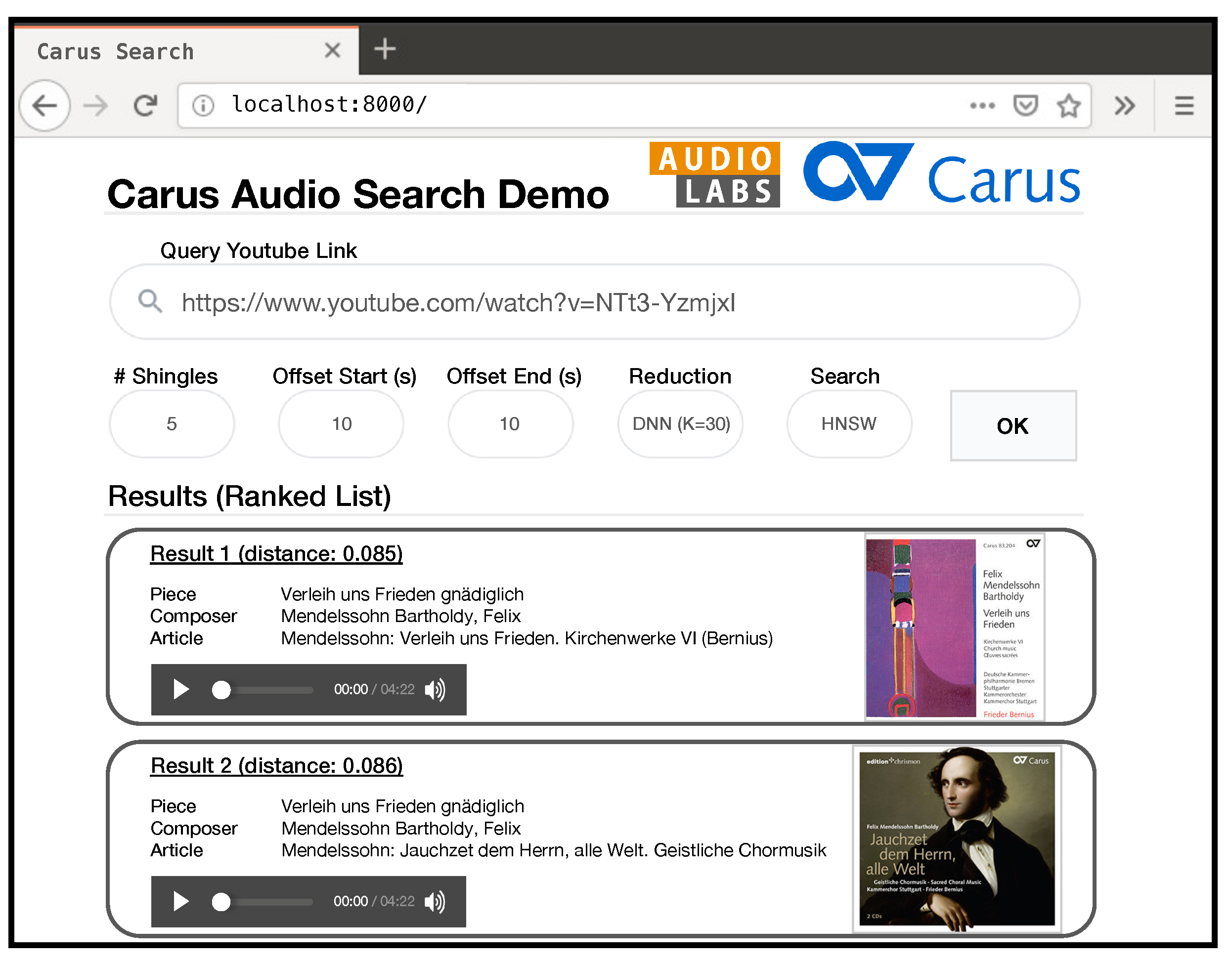
Figure 2.
Illustration of shingle-based query and database document.
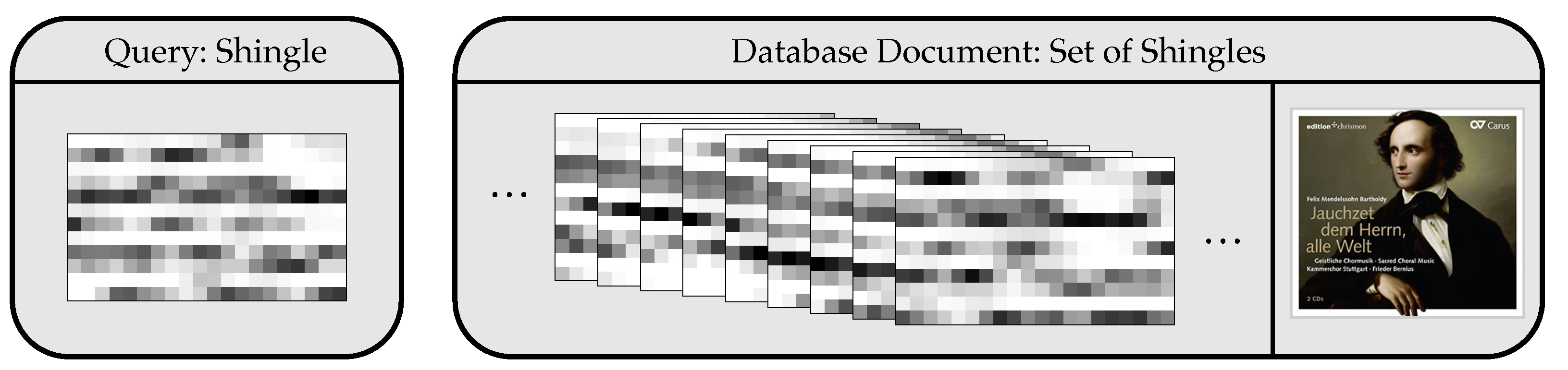
Figure 3.
Illustration of graph-based approximate nearest neighbor search.
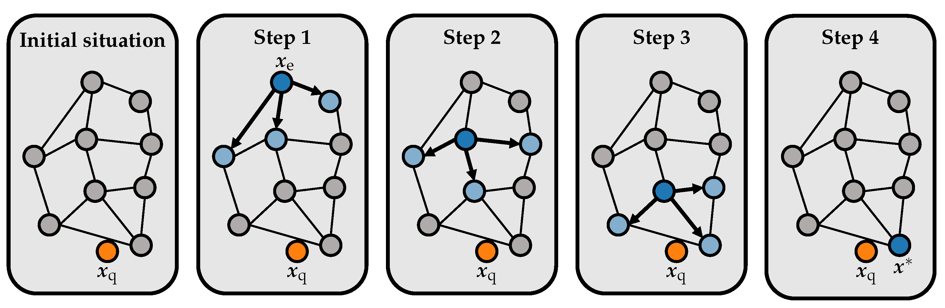
Figure 4.
Illustration of HNSW graph.
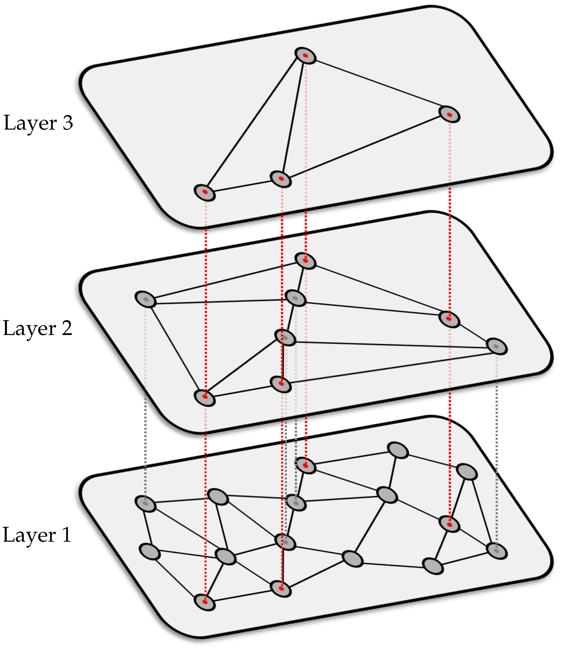
Figure 5.
Search runtimes (in ms) for the DNN- and PCA-based embedding approaches. Note the different scale of the vertical axes. The solid lines show the mean and the light areas show ± the standard deviation around the mean for the repetitions of our experiment. Search using (a) the KD strategy and , (b) the HNSW strategy and , (c) the KD strategy and , and (d) the HNSW strategy and .


Table 1.
Statistics for the used datasets. Duration format hh:mm:ss. Annotations refer to the availability of complete annotations for the musical pieces underlying the recordings (required to evaluate retrieval quality). refers to the total, and ø refers to the average.
Table 1.
Statistics for the used datasets. Duration format hh:mm:ss. Annotations refer to the availability of complete annotations for the musical pieces underlying the recordings (required to evaluate retrieval quality). refers to the total, and ø refers to the average.
| # Audio Files | ∑ Duration | ø Duration | Annotations | # Shingles | |
|---|---|---|---|---|---|
| 330 | 16:13:37 | 0:02:57 | ✓ | 52,332 | |
| 7115 | 389:58:03 | 0:03:17 | ✗ | 1,272,386 |
Table 2.
Considered performance measures.
| Step | Performance Measure | Stage | Section |
|---|---|---|---|
| Overall pipeline | Quality (P@1, P@3, P) | Offline & online | Section 4.2 |
| Feature computation | Time (ms) | Offline & online | Section 4.3 |
| Constructing the index | Time (s) | Offline | Section 4.4 |
| Saving the index | Disk space (MB) | Offline | Section 4.4 |
| Loading the index | Time (ms) | Offline | Section 4.4 |
| Retrieval | Time (ms) | Online | Section 4.5 |
Table 3.
Retrieval quality for various reduction approaches and search strategies using the dataset . Note that the evaluation measures for the KD search approach are identical to the full search approach.
Table 3.
Retrieval quality for various reduction approaches and search strategies using the dataset . Note that the evaluation measures for the KD search approach are identical to the full search approach.
| Reduction | K | Search | P@1 | P@3 | P |
|---|---|---|---|---|---|
| — | 240 | Full Search | 1.0000 | 0.9965 | 0.9434 |
| HNSW | 1.0000 | 0.9965 | 0.9434 | ||
| PCA | 30 | Full Search | 1.0000 | 0.9910 | 0.9130 |
| HNSW | 1.0000 | 0.9910 | 0.9130 | ||
| 12 | Full Search | 1.0000 | 0.9679 | 0.8294 | |
| HNSW | 1.0000 | 0.9678 | 0.8294 | ||
| 6 | Full Search | 1.0000 | 0.8937 | 0.7350 | |
| HNSW | 1.0000 | 0.8937 | 0.7350 | ||
| DNN | 30 | Full Search | 1.0000 | 0.9868 | 0.9344 |
| HNSW | 1.0000 | 0.9869 | 0.9345 | ||
| 12 | Full Search | 1.0000 | 0.9757 | 0.8989 | |
| HNSW | 1.0000 | 0.9756 | 0.8989 | ||
| 6 | Full Search | 1.0000 | 0.9236 | 0.8333 | |
| HNSW | 1.0000 | 0.9237 | 0.8333 |
Table 4.
Time measurements (in ms) for various steps involved in the feature computation of 20 s of audio.
Table 4.
Time measurements (in ms) for various steps involved in the feature computation of 20 s of audio.
| Step | Time (ms) |
|---|---|
| Audio Loading | 44.8 ± 1.4 |
| Spectral Feature Computation | 1171.5 ± 34.3 |
| CENS Feature Computation | 0.9 ± 0.5 |
| Embedding PCA () | 0.05 ± 0.0 |
| Embedding PCA () | 0.05 ± 0.0 |
| Embedding PCA () | 0.05 ± 0.0 |
| Embedding DNN () | 1.6 ± 0.1 |
| Embedding DNN () | 1.5 ± 0.1 |
| Embedding DNN () | 1.4 ± 0.1 |
Table 5.
Performance measures for constructing, saving, and loading the index structure.
| Search | Reduction | K | Construction Time (s) | Save Size (MB) | Load Time (ms) | |||
|---|---|---|---|---|---|---|---|---|
| KD | — | 240 | 0.54 ± 0.0 | 43.03 ± 0.1 | 209.7 | 5161.2 | 131.5 ± 0.4 | 3209.1 ± 25.4 |
| KD | PCA | 30 | 0.06 ± 0.0 | 3.89 ± 0.2 | 27.0 | 664.8 | 17.5 ± 0.3 | 405.1 ± 8.8 |
| KD | PCA | 12 | 0.03 ± 0.0 | 1.66 ± 0.1 | 11.3 | 279.4 | 3.5 ± 0.1 | 167.0 ± 6.9 |
| KD | PCA | 6 | 0.02 ± 0.0 | 0.99 ± 0.1 | 6.1 | 150.9 | 2.1 ± 0.3 | 86.3 ± 2.2 |
| HNSW | — | 240 | 0.65 ± 0.0 | 26.66 ± 0.0 | 53.9 | 1310.9 | 108.1 ± 0.4 | 2680.0 ± 42.8 |
| HNSW | PCA | 30 | 0.51 ± 0.0 | 16.38 ± 0.0 | 9.9 | 241.8 | 85.1 ± 2.1 | 2095.3 ± 6.6 |
| HNSW | PCA | 12 | 0.43 ± 0.0 | 11.58 ± 0.0 | 6.2 | 150.2 | 82.9 ± 0.4 | 2071.5 ± 43.8 |
| HNSW | PCA | 6 | 0.42 ± 0.0 | 10.20 ± 0.0 | 4.9 | 119.6 | 82.6 ± 0.6 | 2049.1 ± 22.8 |
Table 6.
Search runtimes (in ms) using a single query for various dimensions K and search strategies.
Table 6.
Search runtimes (in ms) using a single query for various dimensions K and search strategies.
| Reduction | K | Search | ||||||||
|---|---|---|---|---|---|---|---|---|---|---|
| — | 240 | Full Search | 13.912 | 13.912 | 13.824 | 13.875 | — | — | — | — |
| KD | 0.072 | 23.136 | 24.463 | 25.269 | 771.623 | 775.116 | 770.461 | 772.946 | ||
| HNSW | 0.008 | 0.008 | 0.009 | 0.072 | 0.020 | 0.020 | 0.021 | 0.205 | ||
| PCA | 30 | Full Search | 4.803 | 4.757 | 4.768 | 4.812 | — | — | — | — |
| KD | 0.009 | 0.621 | 1.001 | 2.025 | 36.825 | 48.145 | 66.499 | 88.849 | ||
| HNSW | 0.007 | 0.007 | 0.007 | 0.056 | 0.010 | 0.009 | 0.019 | 0.123 | ||
| PCA | 12 | Full Search | 4.354 | 4.418 | 4.322 | 4.360 | — | — | — | — |
| KD | 0.004 | 0.087 | 0.233 | 0.713 | 0.907 | 1.698 | 4.414 | 10.280 | ||
| HNSW | 0.007 | 0.007 | 0.007 | 0.056 | 0.009 | 0.009 | 0.009 | 0.067 | ||
| PCA | 6 | Full Search | 4.123 | 4.115 | 4.124 | 4.159 | — | — | — | — |
| KD | 0.003 | 0.019 | 0.074 | 0.346 | 0.031 | 0.065 | 0.201 | 0.852 | ||
| HNSW | 0.007 | 0.007 | 0.006 | 0.048 | 0.007 | 0.007 | 0.011 | 0.072 | ||
| DNN | 30 | Full Search | 4.899 | 4.897 | 4.883 | 4.930 | — | — | — | — |
| KD | 0.009 | 0.459 | 1.019 | 2.498 | 30.021 | 46.611 | 75.748 | 117.543 | ||
| HNSW | 0.007 | 0.007 | 0.007 | 0.057 | 0.011 | 0.011 | 0.011 | 0.077 | ||
| DNN | 12 | Full Search | 4.439 | 4.434 | 4.433 | 4.480 | — | — | — | — |
| KD | 0.004 | 0.064 | 0.177 | 0.709 | 0.377 | 0.829 | 2.498 | 7.240 | ||
| HNSW | 0.008 | 0.008 | 0.009 | 0.068 | 0.006 | 0.007 | 0.007 | 0.056 | ||
| DNN | 6 | Full Search | 4.165 | 4.162 | 4.171 | 4.220 | — | — | — | — |
| KD | 0.002 | 0.014 | 0.062 | 0.310 | 0.019 | 0.039 | 0.141 | 0.663 | ||
| HNSW | 0.006 | 0.007 | 0.007 | 0.054 | 0.007 | 0.007 | 0.007 | 0.057 | ||
Publisher’s Note: MDPI stays neutral with regard to jurisdictional claims in published maps and institutional affiliations. |
© 2021 by the authors. Licensee MDPI, Basel, Switzerland. This article is an open access article distributed under the terms and conditions of the Creative Commons Attribution (CC BY) license (https://creativecommons.org/licenses/by/4.0/).
Share and Cite
MDPI and ACS Style
Zalkow, F.; Brandner, J.; Müller, M. Efficient Retrieval of Music Recordings Using Graph-Based Index Structures. Signals 2021, 2, 336-352. https://doi.org/10.3390/signals2020021
AMA Style
Zalkow F, Brandner J, Müller M. Efficient Retrieval of Music Recordings Using Graph-Based Index Structures. Signals. 2021; 2(2):336-352. https://doi.org/10.3390/signals2020021
Chicago/Turabian StyleZalkow, Frank, Julian Brandner, and Meinard Müller. 2021. "Efficient Retrieval of Music Recordings Using Graph-Based Index Structures" Signals 2, no. 2: 336-352. https://doi.org/10.3390/signals2020021