An Educational Guide through the FMP Notebooks for Teaching and Learning Fundamentals of Music Processing

Abstract

This paper provides a guide through the FMP notebooks, a comprehensive collection of educational material for teaching and learning fundamentals of music processing (FMP) with a particular focus on the audio domain. Organized in nine parts that consist of more than 100 individual notebooks, this collection discusses well-established topics in music information retrieval (MIR) such as beat tracking, chord recognition, music synchronization, audio fingerprinting, music segmentation, and source separation, to name a few. These MIR tasks provide motivating and tangible examples that students can hold onto when studying technical aspects in signal processing, information retrieval, or pattern analysis. The FMP notebooks comprise detailed textbook-like explanations of central techniques and algorithms combined with Python code examples that illustrate how to implement the methods. All components, including the introductions of MIR scenarios, illustrations, sound examples, technical concepts, mathematical details, and code examples, are integrated into a unified framework based on Jupyter notebooks. Providing a platform with many baseline implementations, the FMP notebooks are suited for conducting experiments and generating educational material for lectures, thus addressing students, teachers, and researchers. While giving a guide through the notebooks, this paper’s objective is to yield concrete examples on how to use the FMP notebooks to create an enriching, interactive, and interdisciplinary supplement for studies in science, technology, engineering, and mathematics. The FMP notebooks (including HTML exports) are publicly accessible under a Creative Commons Attribution-NonCommercial-ShareAlike 4.0 International License.

1. Introduction

Music information retrieval (MIR) is an exciting and challenging area of research. Music not only connects people but also relates to many different research disciplines, including signal processing, information retrieval, machine learning, musicology, and psychoacoustics. In its beginnings, research in MIR has borrowed many ideas and concepts from more established disciplines such as speech processing or computer linguistics. After more than twenty years, the MIR field has matured to an independent research area, which has many things to offer to signal processing and other research disciplines. Using well-established music analysis and retrieval topics, the textbook on Fundamentals of Music Processing [1] (FMP) yields an example of how music may provide a rich and challenging application domain for introducing, teaching, and studying fundamental techniques and algorithms relevant for general courses in computer science, multimedia engineering, information science, and digital humanities. While providing profound technological knowledge as well as a comprehensive treatment of music processing applications, the book also includes numerous examples and illustrations to convey the main ideas in an intuitive fashion.

In recent years, suitably designed software packages and freely accessible web-based frameworks have made education in computer science and signal processing more interactive. Such novel technology allows for designing courses that help students move from recalling and reciting theoretical concepts towards comprehension and application. These new developments are precisely the motivation for the development of the FMP Notebooks, which provide an interactive foundation for teaching and learning fundamentals of music processing (FMP). The FMP notebooks are built upon the Jupyter notebook framework, which has become a standard in industry as well as in educational settings [2]. This open-source web application allows users to create documents that contain live code, text-based information, mathematical formulas, plots, images, sound examples, and videos. By leveraging the Jupyter framework, the FMP notebooks bridge the gap between theory and practice, where technical concepts and mathematical details are interleaved with code examples, illustrations, and sound examples (see Figure 1). The FMP notebooks closely follow the eight chapters of the textbook [1], and as such, provide an explicit link between structured educational environments and current professional practices, in line with current curricular recommendations for computer science [3].

With this paper, we provide a comprehensive guide through the FMP notebooks. The parts of the FMP notebooks’ main body, as shown in Figure 2, cover MIR topics starting with music representations and Fourier analysis through beat tracking and chord recognition to retrieval and audio decomposition. Each part, in turn, consists of about 10–15 notebooks that provide in-depth descriptions of techniques and algorithms, which are motivated, applied, and evaluated within the given MIR context. While giving a guide through the notebooks, this paper’s main objective is to make concrete suggestions on using the FMP notebooks to create an enriching, interactive and interdisciplinary supplement in the form of experiments and advanced studies in a music processing curriculum. Furthermore, we show how the notebooks allow for generating appealing multimedia objects such as figures and sound examples, which may be useful for lectures and scientific publications. The FMP notebooks are publicly available under a Creative Commons Attribution-NonCommercial-ShareAlike 4.0 International License at https://www.audiolabs-erlangen.de/FMP (accessed on 22 April 2021) in the form of Jupyter notebooks as well as HTML exports, which can be accessed through a conventional web browser. The guide provided by this paper can be best appreciated and understood when the FMP notebooks are opened in a browser simultaneously while reading.

Using the static HTML version, all multimedia material, including the music examples, audio files, video files, and images, can be directly accessed without any specific technical requirements beyond a standard web browser. To execute the FMP notebooks’ code, one needs to install Python, Jupyter, and additional Python packages. All necessary steps for installing, running, and updating the required software packages are described in a separate part (called Part B) of the FMP notebooks. This part also contains short introductions to Python programming, Jupyter notebooks, and multimedia integration while providing functions for data annotation, visualization, and sonification. Rather than being comprehensive, Part B gives instructive code examples that become relevant in the other parts while documenting how the FMP notebooks were created.

The remainder of the paper is organized as follows. In Section 2, we review related software frameworks and toolboxes for audio and music processing. Then, in Section 3, we give an overview of the main technical concepts and required software tools that underlie the FMP notebook while summarizing the content of Part B. The educational guide through the FMP notebooks can be found in Section 4, where the eight parts are organized along with the eight chapters of the textbook [1]. Finally, concluding remarks with pointers for further reading in the area of deep learning can be found in Section 5. While the first sections of this paper are an extended and updated version of the ref. [4] that originally introduced the FMP notebooks, the educational guide in Section 4 is presented here for the first time and constitutes this paper’s main contribution.

2. Related Work

There are a number of excellent and well-document toolboxes that provide modular source code for processing and analyzing music and audio signals. In the following, we give an overview of open-source toolboxes that have been specifically designed for supporting MIR research. We start with prominent examples of code collections for audio and music feature extraction. An early example of such a toolbox is Marsyas, which offers a software framework for rapid prototyping and experimentation with audio analysis and synthesis with specific emphasis to music signals [5]. Similarly, the jAudio toolbox was designed for facilitating easy-to-use audio feature extraction, where the duplication of effort in calculating features from an audio signal is eliminated [6]. The MIRtoolbox consists of an integrated set of MATLAB functions for the extraction of musical features that decscribe tonality, rhythm, and structures from audio files [7]. The Essentia library offers an extensive collection of flexible and easily extendable algorithms for computing a large set of spectral, temporal, tonal, and high-level audio and music descriptors. Written in C++, the library includes Python and JavaScript bindings as well as various command-line tools, which facilitate its use for fast prototyping and allow setting up research experiments rapidly [8]. Recently, the open-source JavaScript (JS) library Essentia.js that allows for efficient and robust real-time audio feature extraction on web browsers was released [9].

There are also various, more specialized toolboxes that focus on specific MIR applications such as the Chroma Toolbox for chroma feature extraction [10], the Constant-Q Toolbox for computing time–frequency transforms [11], the TSM Toolbox for time-scale modification [12], the Tempogram Toolbox for tempo and pulse tracking [13], the NMF toolbox for nonnegative matrix factorization with applications to audio decomposition [14], the SM Toolbox for computing and enhancing similarity matrices, and the MSAF toolbox for audio structure analysis [15]. While most of these toolboxes cover more traditional MIR techniques, the recent Python library madmom offers code for MIR approaches (including onset detection, beat tracking, and chord recognition) that employ deep learning techniques [16]. Furthermore, based on deep learning, Open-Unmix provides an open-source reference implementation for the MIR task of music source separation [17]. Other useful toolboxes provide code for the evaluation of MIR approaches such as the mir_eval library [18] or for data augmentation such as the Audio Degradation Toolbox [19] or the muda library [20].

While most of these toolboxes have been developed especially for research purposes, some of them go along with excellent documentation and example applications that not only illustrate how the code works but also give insights into the underlying techniques and algorithms. We now mention some code collections that have been specially developed for didactic purposes. One such example is the ACA-Code, which is a collection of MATLAB and Python functions accompanying the textbook on Audio Content Analysis [21]. While the book covers the theoretical background for various audio and music processing concepts, the code collection provides corresponding reference implementations that enable students to gain hands-on experience. Based on the Juypter Notebook framework, the MIR Notebooks provided by Steve Tjoa are a collection of instructional MIR materials, containing a mix of casual conversation, technical discussion, and Python code. Similarly, using the Jupyter Book framework, the tutorial on Music Source Separation interleaves textbook-like explanations with code interactively [22]. Last but not least, we want to draw attention to the Python package librosa, which provides basic functions as well as advanced processing pipelines for several music and audio analysis tasks [23]. This package also comprises a gallery of advanced examples, which nicely illustrate how to use the package for approaching MIR tasks such as onset detection, music synchronization, harmonic-percussive separation, and audio structure analysis.

The FMP Notebooks are inspired by librosa and integrate, extend, and complement elements offered by this package. While librosa is designed to be an easy-to-use toolbox with convenient presets, the emphasis of the FMP notebooks is on the educational side, promoting the understanding of MIR concepts. Therefore, rather than providing compact and efficient code, the FMP code examples’ programming style is explicit and straightforward with a flat, functional hierarchy (at the cost of redundancy). The mathematical notation and the naming conventions used in the FMP notebooks are carefully matched to each other, thus establishing a close relationship between theory and practice. Furthermore, the FMP notebooks allow for generating appealing multimedia objects such as figures and sound examples, which may be useful for lectures and scientific publications. In summary, educational and didactic considerations are the leading guide in the development of the FMP notebooks. We hope that these notebooks constitute a useful complement to existing open-source toolboxes while fostering education and research in MIR.

3. Technical Framework (Part B)

This section describes the software framework and central functions that form the technical backbone of the FMP notebooks. These aspects are also covered by Part B—a part which serves different purposes. First, the notebooks of Part B describe the main tools used for developing the FMP notebooks. Second, they give short introductions of the relevant software concepts while providing links to more advanced tutorials. Third, the notebooks give practical advice and examples for generating, using, and integrating code, figures, and sound elements as used throughout the FMP notebooks. In the following, we describe the technical aspects along with the notebooks of Part B. To better understand the explanations, we recommend opening the corresponding notebooks of Part B, which can be accessed as a static HTML version through a standard web browser without any further installation.

3.1. Installation

To obtain a dynamic version of the FMP notebooks, one needs to install Python, Jupyter, and additional Python packages. In the FMP Notebook Get Started, one finds a short introduction on how to get the FMP notebooks run. More detailed explanations can be found in the FMP Notebook Installation, where we introduce the source package manager conda and explain how to use it for installing, running, and updating the required software packages. Furthermore, we provide a file that specifies a Python environment called FMP. This environment file lists all packages (specified by name and version number) needed for the FMP notebooks. Giving a detailed description, we explain how to use the package manager to automatically set up this environment.

3.2. Jupyter Notebook

The FMP notebooks are based on the Jupyter notebook framework. As said before, this open-source web application allows users to create documents that contain live code, text-based information, mathematical formulas, plots, images, sound examples, and videos. Jupyter notebooks are often used as a publishing format for reproducible computational workflows [2]. They can be exported to a static HTML format, making it possible to generate web applications that can be accessed through standard web browsers with no specific technical requirements. The FMP Notebook Jupyter Notebook covers some basic elements of the Jupyter framework, including practical aspects such as essential Jupyter operators and keyboard shortcuts.

3.3. Python

In the FMP notebooks, we use Python as the programming language. The reason for this choice is that Python is an open-source general-purpose language, which is widely used in scientific computing and offers plenty of resources in data sciences and machine learning. Furthermore, being a beginner-friendly language, it suits the didactic orientation of the FMP notebooks well. The FMP Notebook Python Basics contains a short introduction to Python summarizing the most important data types, control structures, and functions as occurring in later parts of the FMP notebooks. One of our design principles is to keep the required programming skills at an elementary level. Furthermore, one finds code examples that illustrate how to create appealing figures, process audio files, and program interactive plots. Furthermore, the FMP Notebook Python Style Guide makes some general recommendations for coding conventions as often used in Python.

3.4. Multimedia

The FMP Notebook Multimedia gives a short overview of how to integrate multimedia objects (in particular, audio, image, and video objects) into a Jupyter notebook. Rather than being comprehensive, we only give a selection of possibilities as used in the other parts of the FMP notebooks. In particular, we discuss two alternatives: a direct integration of images, video, and audio elements using HTML tags as well as an integration using the Python module IPython.display. Python provides powerful functionalities for generating and plotting figures. In the FMP Notebook Python Visualization, we discuss concrete examples on how to generate images to visualize waveforms (audio signals), spectrograms (time–frequency representations), and other feature representations. In doing so, we introduce alternatives based on the Python library matplotlib and the Python package librosa. Furthermore, we discuss how to control the size and position of a colorbar and how to define useful colormaps. Finally, the handling of audio files is covered in the FMP Notebook Python Audio. In particular, we introduce several ways to read and write audio files in Python, using different packages. Furthermore, we discuss the advantages as well as disadvantages of these options.

3.5. Numba

In the FMP Notebook Numba, we give a short introduction to the Python package numba, which offers a just-in-time (JIT) compiler that translates a subset of Python code into fast machine code. Even though not crucial from a functionality point of view, we use this package to significantly speed up (sometimes by a factor of 100) some of our implementations. Rather than being comprehensive, we give some concrete examples (including the option for parallel computing) while highlighting some of the restrictions when using numba.

3.6. Annotation Visualization and Sonification

Annotations of musical properties such as beat positions, structural segments, or chord labels play an essential role when training or testing MIR approaches. Such annotations, which are typically generated by domain experts in a manual process, are often used as reference for evaluating computational methods. In the FMP Notebook Annotation Visualization, we introduce some Python functions for parsing and visualizing various kinds of annotations as encountered in music processing. In particular, we consider single-value annotations (e.g., used to encode beat positions) and segment annotations that consist of pairs of values (e.g., used to encode chord segments). These functions are used throughout the FMP notebooks to explain feature properties and enrich visualizations (see Figure 3 for examples).

The visualization of feature representations along with annotations not only deepens the understanding of signal processing concepts but also provides valuable insights into musical and acoustic properties of the underlying audio signals. As an alternative or complement to data visualization, one may also use data sonification as a means for providing acoustic feedback on the nature of extracted or annotated information. In the FMP Notebook Sonification, we introduce several sonification methods that are helpful in analyzing annotations as well as audio features extracted from a music recording.

3.7. Further Topics and Summary

In Part B, we introduce various Python libraries that are used throughout the FMP notebooks. In particular, in the FMP Notebook libfmp, we give a short introduction on how Python modules and packages are structured. Based on these concepts, we explain how the functions that are systematically developed throughout the various parts of the FMP notebooks are organized to form the Python package libfmp. This packages makes it possible to easily use all the FMP notebooks’ functionality for other projects. Finally, the FMP Notebook MIR Resources contains links to literature, toolboxes, and other resources that may be useful for research in music processing and music information retrieval (MIR). However, we would like to point out that the information provided on this website does not claim to be comprehensive.

In summary, with the notebooks of Part B, our goal is to make the FMP notebooks self-contained. Rather than trying to be comprehensive, we give useful and instructive code examples that become relevant in the other parts. Furthermore, Part B also motivates and documents how the FMP notebooks were created.

4. Educational Guide

The main music processing and MIR topics covered by the FMP notebooks are organized in eight parts, which follow the eight chapters of the textbook on Fundamentals of Music Processing [1]. The notebooks include introductions for each MIR task, provide important mathematical definitions, and describe computational approaches in detail. One primary purpose of the FMP notebooks is to provide audio-visual material as well as Python code examples that implement the computational approaches described in [1]. Additionally, the FMP notebooks provide code that allows users to experiment with parameters and to gain an understanding of the computed results by suitable visualizations and sonifications. These functionalities also make it easily possible to input different music examples and to generate figures and illustrations that can be used in lectures and scientific articles. This way, the FMP notebooks complement and go beyond the textbook [1], where one finds a more mathematically oriented approach to MIR. The following guide is organized along with the eight parts corresponding to the textbook’s chapters. For each part, we start with a short summary of the topic and then go through the part’s notebooks in the same chronological as they occur in the FMP notebooks. To understand the guide’s explanations, it is essential to synchronously open the respective notebook. This can be easily achieved, since we explicitly mention each of the notebook’s title, which is additionally linked in the article’s PDF to the HTML version of the respective notebook.

4.1. Music Representations (Part 1)

Musical information can be represented in many different ways. In ([1], Chapter 1), three widely used music representations are introduced: sheet music, symbolic, and audio representations. The term sheet music is used to refer to visual representations of a musical score either given in printed form or encoded digitally in some image format. The term symbolic stands for any kind of symbolic representation where the entities have an explicit musical meaning. Finally, the term audio is used to denote music recordings given in the form of acoustic waveforms. The boundaries between these classes are not clear. In particular, as illustrated by Figure 4, symbolic representations may be close to both sheet music as well as audio representations [24]. In Part 1 of the FMP notebooks, which is closely associated with the textbook’s first chapter, we introduce basic terminology used throughout the following FMP notebooks. Furthermore, we offer visual and acoustic material as well as Python code examples to study musical and acoustic properties of music, including frequency, pitch, dynamics, and timbre. We now go through the FMP notebooks of Part 1 one by one while indicating how these notebooks can be used for possible experiments and exercises.

We start with the FMP Notebook Sheet Music Representations, where we take up the example of Beethoven’s Fifth Symphony. Besides the piano reduced version and a full orchestral score, we also show a computer-generated sheet music representation. The comparison of these versions is instructive, since it demonstrates the huge differences one may have between different layouts, also indicating that the generation of visually pleasing sheet music representations from score representations is an art in itself. Besides the visual data, the notebook also provides different recordings of this passage, including a synthesized orchestral version created from a full score and a recording by the Vienna Philharmonic orchestra conducted by Herbert von Karajan (1946). The comparison between the mechanical and performed versions shows that one requires additional knowledge not directly specified in the sheet music to make the music come alive. In the data folder of Part 1 (data/C1), one finds additional representations of our Beethoven example including a piano, orchestral, and string quartet version. The files with the extension .sib, which were generated by the Sibelius music notation software application, have been exported in other symbolic formats (.mid, .sib, .xml), image formats (.png), and audio formats (.wav, .mp3). Such systematically generated data is well suited for hands-on exercises that allow teachers and students to experiment within a controlled setting. This is also one reason why we will take up the Beethoven (and other) examples again and again throughout the FMP notebooks.

In the FMP Notebook Musical Notes and Pitches, we deepen the concepts as introduced in ([1], Section 1.1.1). We show how to generate musical sounds using a simple sinusoidal model, which can then be used to obtain acoustic representations of concepts such as octaves, pitch classes, and musical scales. In the FMP Notebook Chroma and Shepard Tones, we generate Shepard tones, which are weighted superpositions of sine waves separated by octaves. These tones can be used to sonify the chromatic circle and Shepard’s helix of pitch as shown in the notebook’s figures. Extending the notion of the twelve-tone discrete chromatic circle, one can generate a pitch-continuous version, where the Shepard tones ascend (or descend) continuously. Originally created by the French composer Jean-Claude Risset, this continuous version is also known as the Shepard–Risset glissando. To implement such a glissando, one requires a chirp function with an exponential (rather than a linear) frequency increase. Experimenting with Shepard tones and glissandi not only leads to interesting sound effects that may be used even for musical compositions but also deepens the understanding of concepts such as frequency, pitch, and the role of overtones. The concept of Shepard tones can also be used to obtain a chromagram sonification as introduced in the FMP Notebook Sonification of Part B.

In the subsequent FMP notebooks, we discuss Python code for parsing, converting, and visualizing various symbolic music formats. In particular, for students who are not familiar with Western music notation, the piano-roll representation yields an easy-to-understand geometric encoding of symbolic music. Motivated by traditional piano rolls, the horizontal axis of this two-dimensional representation encodes time, whereas the vertical axis encodes pitch. The notes are visualized as axis-parallel rectangles, where the color of the rectangles can be used to encode additional note parameters such as velocity or instrumentation (see Figure 5). A piano-roll representation can be easily stored in a comma-separated values (.csv) file, where each line encodes a note event specified by parameters such as start, duration, pitch, velocity, and an additional parameter called label (e.g., encoding the instrumentation). This slim and explicit format, even though representing symbolic music in a simplified way, is used throughout most parts of the FMP notebooks, where the focus is on the processing of waveform-based audio signals. In the FMP Notebook Symbolic Format: CSV, we introduce the Python library pandas, which provides easy-to-use data structures and data analysis tools for parsing and modifying text files. Furthermore, we introduce a function for visualizing a piano-roll representation as shown in Figure 5. The implementation of such visualization functions is an instructive exercise for students to get familiar with fundamental musical concepts as well as to gain experience in standard concepts of Python programming.

As discussed in ([1], Section 1.2), there are numerous formats for encoding symbolic music. Describing and handling these formats in detail goes beyond the FMP notebooks. The good news is that there are various Python software tools for parsing, manipulating, synthesizing, and storing music files. In the FMP Notebook Symbolic Format: MIDI, we introduce the Python package PrettyMIDI for handling MIDI files. This package allows for transforming the (often cryptic) MIDI messages into a list of easy-to-understand note events, which may then be stored using simple .csv files. Similarly, in the FMP Notebook Symbolic Format: MusicXML, we indicate how the Python package music21 can be used for parsing and handling symbolic music given as a MusicXML file. This package is a toolkit for computer-aided musicology allowing users to study large datasets of symbolically encoded music, to generate musical examples, to teach fundamentals of music theory, to edit musical notation, study music and the brain, and to compose music. Finally, in the FMP Notebook Symbolic Format: Rendering, we discuss some software tools for rendering sheet music from a given symbolic music representation. By mentioning a few open-source tools, our notebooks only scratch the surface on symbolic music processing and are intended to yield entry points to this area.

The next FMP notebooks cover aspects of audio representations and their properties following ([1], Section 1.3). In the FMP Notebook Waves and Waveforms, we provide functions for simulating transverse and longitudinal waves as well as combinations thereof. Furthermore, one finds Python code for generating videos of these simulations, thus indicating how the FMP notebooks can be used for generating educational material (see Figure 6). In the FMP Notebook Frequency and Pitch, we discuss some experiments on the audible frequency range and the just-noticeable difference in pitch perception. In the FMP Notebook Harmonic Series, one finds an acoustic comparison of the musical scale based on harmonics with the twelve-tone equal-tempered scale. Similarly, the FMP Notebook Pythagorean Tuning considers the Pythagorean scale. In both of these notebooks, we again use simple sinusoidal models for the sonification. The FMP Notebook Dynamics, Intensity, and Loudness yields an implementation for visualizing the sound power level over time for our Beethoven example. Furthermore, we present an experiment using a chirp signal to illustrate the relation between signal power and perceived loudness. In the FMP Notebook Timbre, we introduce simple yet instructive experiments that are also suitable as programming exercises. First, we give an example on how one may compute an envelope of a waveform by applying a windowed maximum filter. Then, we provide some implementations for generating synthetic sinusoidal signals with vibrato (frequency modulations) and tremolo (amplitude modulations). Finally, we demonstrate that the perception of the perceived pitch depends not only on the fundamental frequency but also on its higher harmonics and their relationships. In particular, we show that a human may perceive the pitch of a tone even if the fundamental frequency associated to this pitch is completely missing.

In summary, the FMP notebooks of Part 1 provide basic Python code examples for parsing and visualizing various music representations. Furthermore, we consider tangible music examples and suggest various experiments for gaining a deeper understanding of musical and acoustic properties of audio signals. At the same time, the material is also intended for developing Python programming skills as required in the subsequent FMP notebooks.

4.2. Fourier Analysis of Signals (Part 2)

The Fourier transform is undoubtedly one the most fundamental tools in signal processing, and it plays a central role also throughout all parts of the FMP notebooks. In ([1], Chapter 2), the Fourier transform is approached from various perspectives considering real-valued and complex-valued versions as well as analog and discrete signals. The underlying idea is to analyze a given signal by means of elementary sinusoidal (or exponential) functions, which possess an explicit physical meaning in terms of frequency. The Fourier transform converts a time-dependent signal into frequency-dependent coefficients, each of which indicates the degree of correlation between the signal and the respective elementary sinusoidal function. The process of decomposing a signal into frequency components is also called Fourier analysis. In contrast, the Fourier representation shows how to rebuild a signal from the elementary functions, a process also called Fourier synthesis. In Part 2 of the FMP notebooks, we approach Fourier analysis from a practical perspective with a focus on the discrete Fourier transform (DFT). In particular, we cover the entire computational pipeline in a bottom-up fashion by providing Python code examples for deepening the understanding of complex numbers, exponential functions, the DFT, the fast Fourier transform (FFT), and the short-time Fourier transform (STFT). In this context, we address practical issues such as digitization, padding, and axis conventions—issues that are often neglected in theory. Assuming that the reader has opened the FMP notebooks of Part 2, we now briefly comment on the FMP notebooks in the order in which they appear.

We start with the FMP Notebook Complex Numbers, where we review basic properties of complex numbers. In particular, we provide Python code for visualizing complex numbers using either Cartesian coordinates or polar coordinates. Such visualizations help students gain a geometric understanding of complex numbers and the effect of their algebraic operations. Subsequently, we consider in the FMP Notebook Exponential Function the complex version of the exponential function. Many students are familiar with the real version of this function, which is often introduced by its power series

$$exp\left(a\right)=\sum _{n=0}^{\infty }{a}^n/n!$$

for $a\in \mathbb{R}$ This definition can be extended by replacing the real variable $a\in \mathbb{R}$ by a complex variable $c\in \mathbb{C}$. Studying the approximation quality of the power series (and other limit definitions of the exponential function) is instructive and can be combined well with small programming exercises. One important property of the complex exponential function, which is also central for the Fourier transform, is expressed by Euler’s formula $exp\left(i\gamma \right)=cos\left(\gamma \right)+isin\left(\gamma \right)$ for $\gamma \in \mathbb{R}$. We provide a visualization that illustrates how the exponential function restricted to the unit circle relates to the real sine and cosine functions. Furthermore, we discuss the notion of roots of unity, which are the central building blocks that relate the exponential function to the DFT matrix. The study of these roots can be supported by small programming exercises, which may also cover mathematical concepts such as complex polynomials and the fundamental theorem of algebra.

In the FMP Notebook Discrete Fourier Transform, we approach the DFT in various ways. Given an input vector $x={(x\left(0\right),x\left(1\right),\dots ,x(N-1))}^{\top }\in {\mathbb{R}}^N$ of length $N\in \mathbb{N}$, the DFT is defined by

$$X\left(k\right):=\sum _{n=0}^{N-1}x\left(n\right)exp(-2\pi ikn/N)$$

for $k\in [0:N-1]$. The output vector $X\in {\mathbb{C}}^N$ can be interpreted as a frequency representation of the time-domain signal x. The real (imaginary) part of a Fourier coefficient $X\left(k\right)$ can be interpreted as the inner product of the input signal x and a sampled version of the cosine (sine) function of frequency $k/N$. In our notebook, we provide a concrete example that illustrates how this inner product can be interpreted as the correlation between a signal x and the cosine (sine) function. We recommend that students experiment with different signals and frequency parameters k to deepen the intuition of these correlations. From a computational view, the vector X can be expressed by the product of the matrix ${\mathrm{DFT}}_N$ with the vector x. Defining the complex number ${\sigma }_N:=\exp (-2\pi i/N)$ (which is a specific root of unity), one can express the DFT matrix in a very compact form given by ${\mathrm{DFT}}_N(n,k)={\sigma }_N^{nk}$ for $n,k\in [0:N-1]$. Visualizing the real and imaginary parts of the DFT matrix reveals its structural properties (see Figure 7). In particular, one can observe that the rows of the DFT matrix correspond to sampled cosine (real part) and sine (imaginary part) functions. The specific structure of the matrix ${\mathrm{DFT}}_N$ (with its relation to ${\mathrm{DFT}}_M$ for $M=N/2$) can be exploited in a recursive fashion, yielding the famous fast Fourier transform (FFT). In our notebook, we provide an explicit implementation of the FFT algorithm and present some experiments, where we compare the running time of a naive implementation with the FFT-based one. We think that implementing and experimenting with the FFT—an algorithm of great beauty and high practical relevance—is a computational eye opener and a must in every signal processing curriculum. Computing a DFT results in complex-valued Fourier coefficients, where each such coefficient can be represented by a magnitude and a phase component. In the FMP Notebook DFT: Phase, we provide a Python code example that highlights the optimality property of the phase. Studying this property is the core of understanding the role of the phase—a concept that is often difficult to access for students new to the field.

Another central topic of signal processing is the short-time Fourier transform (STFT), which is covered in ([1], Section 2.5) for the analog and discrete case. In the FMP Notebook Discrete Short-Time Fourier Transform (STFT), we implement a discrete version of the STFT from scratch and discuss various options for visualizing the resulting spectrogram. While the main idea of the STFT, where one applies a sliding window technique and computes for each windowed section a DFT, seems simple, computing the discrete STFT in practice can be tricky. In an applied signal processing course, it is essential to make students aware of the different parameters and conventions when applying windowing. Our notebooks provide Python implementations that allow students to experiment with the STFT (applied to synthetic signals and real music recordings) and to gain an understanding on how to physically interpret discrete objects such as samples, frames, and spectral coefficients. In the FMP Notebook STFT: Influence of Window Function, we explore the role of the window type and window size. Furthermore, in the FMP Notebook STFT: Padding, we discuss various padding conventions that become crucial to correctly interpret and visualize feature representations. This important topic, which is a typical source of inaccuracies and errors in music processing pipelines, is illustrated by simple examples as a basis for further exploration (see also Figure 8).

One main limitation of the discrete STFT is the linear frequency grid whose resolution is determined by the signal’s sampling rate and the STFT window size. In the FMP Notebook STFT: Frequency Grid Density, we deepen the understanding on the connection between the different parameters involved. In particular, we discuss how to make the frequency grid denser by suitably padding the windowed sections in the STFT computation. Often, one loosely says that this procedure increases the frequency resolution. This, however, is not true in a qualitative sense, as is explained in the notebook. As an alternative, we discuss in the FMP Notebook STFT: Frequency Interpolation another common procedure to adjust the frequency resolution. On the way, we give a quick introduction to interpolation and show how the Python package scipy can be applied for this task. Beside refining the frequency grid, we then show how interpolation techniques can be used for a non-linear deformation of the frequency grid, resulting in a log-frequency spectrogram. This topic goes beyond the scope of the current part, but plays an important role in designing musical features (see, e.g.,  [1], Section 3.1.1).

The matrix ${\mathrm{DFT}}_N$ is invertible, and its inverse ${\mathrm{DFT}}_N^{-1}$ coincides with the DFT matrix up to some normalizing factor and complex conjugation. This algebraic property can be proven using the properties of the roots of unity. In the FMP Notebook STFT: Inverse, we show that the two matrices are indeed inverse to each other—up to some numerical issues due to rounding in floating-point arithmetic. While inverting the DFT is straightforward, the inversion of the discrete STFT is less obvious, since one needs to compensate for effects introduced by the sliding window technique. In our notebook, we provide some basic Python implementation of the inverse STFT since it sheds another light on the sliding windowing concept and its effects. Furthermore, we discuss numerical issues as well as typical errors that may creep into one’s source code when loosing sight of windowing and padding conventions. At this point, we want to emphasize again that the STFT is one of the most important tools in music and audio processing. Common software packages for audio processing offer STFT implementations, including convenient presets and functions for physically interpreting time, frequency, and magnitude parameters. From a teaching perspective, we find it crucial to exactly understand the role of the STFT parameters and the conventions made implicitly in black-box implementations. In the FMP Notebook STFT: Conventions and Implementations, we summarize various variants for computing and interpreting a discrete STFT, while fixing the conventions used throughout the FMP notebooks (if not specified otherwise explicitly).

The FMP notebooks of Part 2 close with some experiments related to the digitization of waveforms and its effects (see also [1], Section 2.2.2). In the FMP Notebook Digital Signals: Sampling, we implement the concept of equidistant sampling and apply it to a synthetic example. We then reconstruct the signal from its samples (using the interpolation of the sampling theorem based on the sinc function) and compare the result with the original signal. Based on the provided functions, one simple yet instructive experiment is to successively decrease the sampling rate and to look at the properties of the reconstructed signal Similarly, starting with a real music recording (e.g., in the notebook, we use a C-major scale played on a piano), students may acoustically explore and understand aliasing effects. We continue with the FMP Notebook Digital Signals: Quantization, where we have a closer look at the effects resulting from quantization. We provide a function for uniform quantization, which is then applied to a synthetic example and visually explored using different quantization parameters. Furthermore, using again the C-major scale recording, we reconstruct an analog signal from the quantized version, which allows for understanding the distortions introduced by quantization (also referred to as quantization noise). We finally introduce an approach for nonuniform quantization, where quantization levels are spaced in a logarithmic fashion. Besides theoretical explanations, we provide Python code that allows students to experiment, compare, and explore the various quantization strategies and their properties (see Figure 9). In the subsequent FMP Notebook Interference and Beating, we pick up the topic of interference, which occurs when a wave is superimposed with another wave of similar frequency. In particular, we present several experiments using sinusoidal as well as chirp functions to visually and acoustically study the related effect of beating.

4.3. Music Synchronization (Part 3)

The objective of music synchronization is to identify and link semantically corresponding events present in different versions of the same underlying musical work. Using this task as a motivating scenario, two problems of fundamental importance to music processing are discussed in ([1], Chapter 3): feature extraction and sequence alignment. In Part 3 of the FMP notebooks, we provide and explain Python code examples of all the components that are required to realize a basic music synchronization pipeline. In the first notebooks, we consider fundamental feature design techniques such as frequency binning, logarithmic compression, feature normalization, feature smoothing, tuning, and transposition. Then, we provide an implementation of an important alignment algorithm known as dynamic time warping (DTW), which was originally used for speech recognition [25], and introduce several experiments for exploring this technique in further depth. Finally, we close Part 3 with a more comprehensive experiment on extracting tempo curves from music recordings, which nicely illustrates the many design choices, their impact, and the pitfalls one has to deal with in a complex audio processing task.

We start with the FMP Notebook Log-Frequency Spectrogram and Chromagram, which provides a step-by-step implementation for computing the log-frequency spectrogram as described in ([1], Section 3.1.1). Even though logarithmic frequency pooling as used in this approach has major drawbacks, it is instructive from an educational point of view. First, students gain a better understanding on how to interpret the frequency grid introduced by a discrete STFT. Second, the pooling strategy reveals the problems associated with the insufficient frequency resolution for low pitches. In our notebook we make this problem explicit by considering a log-frequency spectrogram with empty pitch bins, leading to horizontal artifacts in our chromatic scale example. In the next step, we convert a log-frequency spectrogram into a chromagram by identifying pitches that share the same chroma. In a music processing course, it is an excellent exercise to let students compute and analyze the properties of chromagrams for music recordings of their own choice. This exploration can be done either visually, as demonstrated by our explicit music examples, or acoustically using suitable sonification procedures as provided by the FMP Notebook Sonification of Part B. We close this notebook by discussing alternative variants of log-frequency spectrograms and chromagrams. In the subsequent notebooks, we often employ more elaborate chromagram implementations as provided by the Python package librosa.

Using spectrograms and chromagrams as instructive examples, we explore in the subsequent notebooks the effect of standard feature processing techniques. In the FMP Notebook Logarithmic Compression, the discrepancy between large and small magnitude values is reduced by applying a suitable logarithmic function. To understand the effects of logarithmic compression, it is instructive to experiment with sound mixtures that contain several sources at different sound levels (e.g., a strong drum sound superimposed with a soft violin sound). In the FMP Notebook Feature Normalization, we introduce different strategies for normalizing a feature representation, including the Euclidean norm (${\ell }^2$), the Manhattan norm (${\ell }^1$), the maximum norm (${\ell }^{max}$), and the standard score (using mean and variance). Furthermore, we discuss different strategies for how one may handle small values (close to zero) in the normalization. This notebook is also well suited for practicing the transition from mathematical formulas to implementations. While logarithmic compression and normalization increase the robustness to variations in timbre or sound intensity, we study in the FMP Notebook Temporal Smoothing and Downsampling postprocessing techniques that can be used for making a feature sequence more robust to variations in aspects such as local tempo, articulation, and note execution. We consider two feature smoothing techniques, one based on local averaging and the other on median filtering. Using chroma representations of different recordings of Beethoven’s Fifth Symphony (one of our favorite examples throughout the FMP notebooks), we study smoothing effects and the role of the filter length. Finally, we introduce downsampling as a simple means to decimate the feature rate of a smoothed representation.

The FMP Notebook Transposition and Tuning covers central aspects of great musical and practical importance. As discussed in ([1], Section 3.1.2.2), a musical transposition of one or several semitones can be simulated on the chroma level by a simple cyclic shift. We demonstrate this in the notebook using a C-major scale played on a piano. While transpositions are pitch shifts on the semitone level, we next discuss global frequency deviations on the sub-semitone level. Such deviations may be the result of instruments that are tuned lower or higher than the expected reference pitch $\mathrm{A}4$ with center frequency $440\mathrm{Hz}$. In the case that the tuning deviation is known, one can use this information to adjust the center and cutoff frequencies of the MIDI pitches for computing the log-frequency spectrogram and the chromagram. Estimating the tuning deviation, however, can be quite tricky. One way to introduce this topic in a music processing class is to let students perform, record, and analyze their own music. What is the effect when detuning a guitar or violin? How does strong vibrato affect the perception of pitch and tuning? What happens if the tuning changes throughout the performance? Having such issues in mind, developing and implementing a tuning estimation system can be part of an exciting and instructive student project. In this notebook, we present such a system that outputs a single number $\theta$ between $-50$ and $+50$ yielding the global frequency deviation (given in cents) on the sub-semitone level. In our approach, as illustrated by Figure 10, we first compute a frequency distribution from the given music recording, where we use different techniques such as the STFT, logarithmic compression, interpolation, local average subtraction, and rectification. The resulting distribution is then compared with comb-like template vectors, each representing a specific tuning. The template vector that maximizes the similarity to the distribution yields the tuning estimate. Furthermore, we conduct in the notebook various experiments that illustrate the benefits and limitations of our approach, while confronting the student with the various challenges one encounters when dealing with real music data.

In the next notebooks, closely following ([1], Section 3.2), we cover the second main topic of Part 3, dealing with alignment techniques. In the FMP Notebook Dynamic Time Warping (DTW), we provide an implementation of the basic DTW algorithm. This is a good opportunity for pointing out an issue one often faces in programming. In mathematics and some programming languages (e.g., MATLAB), one uses the convention that indexing starts with the index 1. In other programming languages such as Python, however, indexing starts with the index 0. Neither convention is good or bad. In practice, one needs to make adjustments in order to comply with the respective convention. Implementing the DTW algorithm is a good exercise to make students aware of this issue, which is often a source of programming errors. The FMP Notebook DTW Variants investigates the role of the step size condition, local weights, and global constraints. Rather than implementing all these variants from scratch, we employ a function from the Python package librosa and discuss various parameter settings. Finally, in the FMP Notebook Music Synchronization, we apply the DTW algorithm in the context of our music synchronization scenario. Considering two performances of the beginning of Beethoven’s Fifth Symphony (first twenty measures), we first convert the music recordings into chromagrams, which are then used as input to the DTW algorithm. The resulting warping path constitutes our synchronization result, as shown in Figure 11.

Concluding Part 3 of the FMP notebooks, we provide additional material for some music synchronization applications (see also [1], Section 3.3). In the FMP Notebook Application: Music Navigation, one finds two videos that illustrate the main functionalities of the Interpretation Switcher and Score Viewer Interface. Then, in the FMP Notebook Application: Tempo Curves, we present an extensive experiment for extracting tempo information from a given music recording. Besides the recorded performance, one requires a score-based reference version, which we think of as a piano-roll representation with a musical time axis (given in measures and beats). On the basis of chroma representations, we apply DTW to compute a warping path between the performance and the score. Then, the idea is to compute the slope of the warping path and to take its reciprocal to derive the local tempo. In practice, however, this becomes problematic when the warping path runs horizontally (slope is zero) or vertically (slope is infinite). In the notebook, we solve this issue by thinning out the warping path to enforce strict monotonicity in both dimensions and then continue as indicated before. To make the overall procedure more robust, we also apply a local smoothing strategy in the processing pipeline. Our overall processing pipeline not only involves many steps with a multitude of parameters, but is also questionable from a musical point of view. Using the famous romantic piano piece “Träumerei” by Robert Schumann as a concrete real-world example, we discuss two conflicting goals. On the one hand, the tempo estimation procedure should be robust to local outliers that are the result of computational artifacts (e.g., inaccuracies of the DTW alginment). On the other hand, the procedure should be able to adapt to continuous tempo fluctuations and sudden tempo changes, being characteristic features of expressive performances. Through studying tempo curves and the way they are computed, one can learn a lot about the music as well as computational approaches. Furthermore, this topic leads students to challenging and interdisciplinary research problems.

4.4. Music Structure Analysis (Part 4)

Music structure analysis is a central and well-researched area within MIR. The general objective is to segment a symbolic music representation or an audio recording with regard to various musical aspects, for example, identifying recurrent themes or detecting temporal boundaries between contrasting musical parts. Being organized in a hierarchical way, structure in music arises from various relationships between its basic constituent elements. The principles used to create such relationships include repetition, contrast, variation, and homogeneity [26]. In Part 4 of the FMP notebooks, we approach the core concepts covered in ([1], Chapter 4) from a practical perspective, which are applicable beyond the music domain. In particular, we have a detailed look at the properties and variants of self-similarity matrices (SSMs). Then, considering some more specific music structure analysis tasks, we provide and discuss implementations of—as we think—some beautiful and instructive approaches for repetition and novelty detection. Using real-world music examples, we draw attention to the algorithms’ strengths and weaknesses, while indicating the problems that typically arise from violations of the underlying model assumptions. We close Part 4 by implementing and discussing evaluation metrics, which we take up again in other parts of the FMP notebooks.

We start with the FMP Notebook Music Structure Analysis: General Principles, where we create the general context of the subsequent notebooks of this part. In particular, we introduce our primary example used throughout these notebooks: Brahms’ famous Hungarian Dance No. 5 (see also Figure 12). Based on this example, we introduce implementations for parsing, adapting, and visualizing reference annotations for musical structures. Furthermore, we provide some Python code examples for converting music recordings into MFCC-, tempo-, and chroma-based feature representations. In a music processing course, we consider it essential to make students aware that such representations crucially depend on parameter settings and design choices. This fact can be made evident by suitably visualizing the representations. In the FMP notebooks in general, we attach great importance to a visual representation of results, which sharpens one’s intuition and provides a powerful tool for questioning the results’ plausibility.

One general idea to study musical structures and their mutual relations is to convert the music signal into a suitable feature sequence and compare each element of the feature sequence with all other sequence elements. This results in an SSM, a tool that is of fundamental importance not only for music structure analysis but also for analyzing many kinds of time series. Closely following ([1], Section 4.2), we cover this fundamental topic in the subsequent notebooks. The FMP Notebook Self-Similarity Matrix (SSM) explains the general ideas of SSMs and discusses basic notions such as paths and blocks. Furthermore, continuing our Brahms example, we provide Python code examples for computing and visualizing SSMs using different feature representations. It is an excellent exercise to turn the tables and to start with a structural description of a piece of music and then to transform this description into an SSM representation. This is what we do in the FMP Notebook SSM: Synthetic Generation, where we provide a function for converting a reference annotation of a music recording into an SSM. In this function, one can specify if the structural parts fulfill path-like (being repetitive) or block-like (being homogeneous) relations. Further parameters allow for modifying the SSM by applying a Gaussian smoothing filter or adding Gaussian noise (see Figure 12 for examples). Synthetically generating and visualizing SSMs is a very instructive way to gain a deeper understanding of these matrices’ structural properties and their relation to musical annotations. Furthermore, synthetic SSMs are useful for debugging and testing automated procedures for music structure analysis. However, synthetic SSMs should not replace an evaluation based on real music examples. In practice, SSMs computed from music and audio representations are typically far from being ideal—a painful experience that every student should have.

Subsequently, we consider various strategies for enhancing the structural properties of SSMs. In the FMP Notebook SSM: Feature Smoothing, we study how feature smoothing affects structural properties of an SSM, using our Brahms example as an illustration. For example, starting with a chroma representation and increasing the smoothing length, one may observe an increase in homogeneity reflecting the rough harmonic content. As an alternative to average filtering, we also discussed median filtering. In the FMP Notebook SSM: Path Enhancement, we discuss a strategy for enhancing path structures in SSMs. We show that simple filtering along the main diagonal works well if there are no relative tempo differences between the segments to be compared. Rather than directly implementing this procedure using nested loops, we provide a much faster matrix-based implementation, which exploits efficient array computing concepts provided by the Python package numpy. In a music processing course, this is an excellent opportunity for discussing efficiency and implementation issues. In this context, one may also discuss Python packages such as numba that translate specific Python code into fast machine code. After this little excursion on efficiency, we come back to our Brahms example, where the shorter $B_2$-section is played much faster than the $B_1$-section, leading to non-diagonal path structures (see Figure 12). Here, diagonal smoothing fails, and we introduce a multiple filtering approach that preserves specific non-diagonal structures [27]. Again, rather than implementing this approach in a naive fashion, we employ a matrix-based implementation using a tricky resampling strategy. Finally, we introduce a forward–backward smoothing approach that attenuates fading artifact, in particular at the end of path structures.

In the song “In the Year 2525” by Zager and Evans, certain musical parts are repeated in a transposed form. In the FMP Notebook SSM: Transposition Invariance, we provide an implementation for computing a transposition invariant SSM [28]. In particular, we show how the resulting transposition index matrix can be visualized. Such visualizations are—as we think—aesthetically beautiful and say a lot about the harmonic relationships within a song. We close our studies on SSMs with the  FMP Notebook SSM: Thresholding, where we discuss global and local thresholding strategies, which are applicable to a wide range of matrix representations. The effect of different thresholding techniques can be nicely illustrated by small toy examples, which can also be integrated well into a music processing course in the form of small handwritten and programming exercises.

We now turn our attention to more concrete subtasks of music structure analysis. In the comprehensive FMP Notebook Audio Thumbnailing, we provide a step-by-step implementation of the procedure described in ([1], Section 4.3). This is more of a notebook for advanced students who want to see how the mathematically rigorous description of an algorithm (in this case, the original procedure is presented in [29]), is put into practice. By interleaving theory, implementation details, and immediate application to a specific example, we hope that this notebook gives a positive example of making a complex algorithm more accessible. As the result of our audio thumbailing approach, we obtain a fitness measure that assigns to each possible segment a fitness value. The FMP Notebook Scape Plot Representation introduces a concept for visualizing the fitness values of all segments using a triangular image. This concept is an aesthetically pleasing and powerful way to visualize segment properties in a compact and hierarchical form. Applied to our fitness measure, we deepen the understanding of our thumbnailing procedure by providing scape plot representations for the various measures involved (e.g., score, normalized score, coverage, normalized coverage, and fitness). From a programming perspective, this notebook also demonstrates how to create elaborate illustrations using the Python library matplotlib.

Next, following ([1], Section 4.4), we deal with the music structure analysis subtask often referred to as novelty detection. In the FMP Notebook Novelty-Based Segmentation, we cover the classical and widely used approach originally suggested by Foote [30]. We provide Python code examples for generating box-like and Gaussian checkerboard kernels, which are then shifted along the main diagonal of an SSM to detect 2D corner points. We think that this simple, beautiful, explicit, and instructive approach should be used as a baseline for any research in novelty-based segmentation before applying more intricate approaches. Of course, as we also demonstrate in the notebook, the procedure crucially depends on design choices and parameters such as the underlying SSM and the kernel size.

While most approaches for novelty detection use features that capture local characteristics, we consider in the FMP Notebook Structure Feature the concept of structure features that capture global structural properties [31]. These features are basically the columns of an SSM’s cyclic time–lag representation. In the notebook, we provide an implementation for converting an SSM into a time–lag representation. We also offer Python code examples that students can use to explore this conversion by experimenting with explicit toy examples. Again it is crucial to also apply the techniques to real-world music recordings, which behave completely differently compared with synthetic examples. In practice, one often obtains significant improvements by applying median filtering to remove undesired outliers or by applying smoothing filters to make differentiation less vulnerable to small deviations.

We close Part 4 with the FMP Notebook Evaluation, where we discuss standard metrics based on precision, recall, and F-measure. Even though there are Python libraries such as mir_eval [18] that provide a multitude of metrics commonly used in MIR research, it is essential to exactly understand how these metrics are defined. Furthermore, requiring knowledge in basic data structures and data handling, students may improve their programming skills when implementing, adapting, and applying some of these metrics. In our notebook, one finds Python code examples for the standard precision, recall, and F-measure as well as adaptions of these measures for labeling and boundary evaluation. Again, we recommend using suitable toy examples and visualizations to get a feel for what the metrics actually express.

4.5. Chord Recognition (Part 5)

Another essential and long-studied MIR task is the analysis of harmonic properties of a piece of music by determining an explicit progression of chords from a given music representation—a task often referred to as automatic chord recognition. Following ([1], Chapter 5), we consider a simplified scenario, where only the minor and major triads as occurring in Western music are considered. Assuming that the piece of music is given in the form of an audio recording, the chord recognition task consists in splitting up the recording into segments and assigning a chord label to each segment. The segmentation specifies the start and end time of a chord, and the chord label specifies which chord is played during this time period (see Figure 13). In Part 5 of the FMP notebooks, we provide and discuss Python code examples of all the components that are required to realize a template-based and an HMM-based chord recognizer. Based on evaluation metrics and suitable time–chord representations, we quantitatively and qualitatively discuss how the various components and their parameters affect the chord recognition results. To this end, we consider real-world music recordings, which expose the weaknesses of the automatic procedures, the problem modeling, and the evaluation metrics.

The first notebooks of Part 5 mainly provide sound examples of basic musical notions such as intervals, chords, and scales with a focus on Western tonal music. In the FMP Notebook Intervals, we provide Python code examples for generating sinusoidal sonifications of intervals. We then generate sound examples of the various music intervals with respect to equal temperament, just intonation, and Pythagorean tuning. Besides a mathematical specification of deviations (given in cents), the sound examples allow for an acoustic comparison of intervals generated based on the different intonation schemes. Similarly, in the FMP Notebook Chords, we give sound examples for different chords. In particular, we provide a piano recording as well as a synthesized version of each of the twelve major and minor triads. Finally, in the FMP Notebook Musical Scales and Circle of Fifths, we cover the notions of musical scales and keys. In particular, we look at diatonic scales, which are obtained from a chain of six successive perfect fifth intervals and can be arranged along the circle of fifths. In summary, these three notebooks show how simple sonifications may help to better understand musical concepts. In a music processing course, one may develop small tools for ear training in basic harmony analysis as part of student projects.

After the musical warm-up in the previous notebooks, we introduce in the FMP Notebook Template-Based Chord Recognition a simple yet instructive chord recognizer. For illustration, we use the first measures of the Beatles song “Let It Be” (see Figure 13), which is converted into a chroma representation. As we already discussed in the context of music synchronization, there are many different ways of computing chroma features. As examples, we compute and visualize three different chroma variants as provided by the Python package librosa. Furthermore, we provide Python code examples to generate chord templates, compare the templates against the recording’s chroma vectors in a frame-wise fashion, and visualize the resulting similarity values in the form of a time–chord representation. By looking at the template that maximizes the similarity value, one obtains the frame-wise chord estimate, which we visualize in the form of a binary time–chord representation (see Figure 13c). Finally, we discuss these results by visually comparing them with manually generated chord annotations. We recommend that students also use the functionalities provided by the FMP Notebook Sonification of Part B to complement the visual inspections by acoustic ones. We think that qualitative inspections—based on explicit music examples and using visualizations and sonifications of all intermediate results—are essential for students to understand the technical components, to become aware of the model assumptions and their implications, and to sharpen their intuition of what to expect from computational approaches.

Besides a qualitative investigation using explicit examples and visualizations, one also requires quantitative methods to evaluate an automatic chord recognizer’s performance. To this end, one typically compares the computed result against a reference annotation. Such an evaluation, as we discuss in the FMP Notebook Chord Recognition Evaluation, gives rise to several questions. How should the agreement between the computed result and the reference annotation be quantified? Is the reference annotation reliable? Are the model assumptions appropriate? To what extent do violations of these assumptions influence the final result? Such issues should be kept in mind before turning to specific metrics. Our evaluation focuses on some simple metrics based on precision, recall, and F-measure, as we already encountered in the FMP Notebook Evaluation of Part 4. Before the evaluation, one needs to convert the reference annotation into a suitable format that conforms with the respective metric and the automatic approach’s format. Our notebook demonstrates how one may convert a segment-wise reference annotation (where segment boundaries are specified in seconds) into a frame-wise format. Furthermore, one may need to adjust the chords and naming conventions. All these conversion steps are, by far, not trivial and often require simplifying design choices (similar to the ones illustrated by Figure 12). Continuing our Beatles example, we discuss such issues and make them explicit using suitable visualizations. Furthermore, we address some of the typical evaluation problems that stem from chord ambiguities (e.g., due to an oversimplification of the chord models) or segmentation ambiguities (e.g., due to broken chords). We hope that this notebook is a source of inspiration for students to conduct experiments with their own music examples.

Motivated by the chord recognition problem, the FMP Notebook Hidden Markov Model (HMM) deepens the understanding of this important sequence analysis technique, which was originally applied to speech recognition [32]. Closely following ([1], Section 5.3), we start by providing a Python function that generates a state and observation sequence from a given discrete HMM. Conversely, knowing an observation sequence as well as the underlying state sequence it was generated from (which is normally hidden), we show how one can estimate the state transition and output probability matrices. The general problem of estimating HMM parameters only on the basis of observation sequences is much harder. An iterative procedure that finds a locally optimal solution is known as the Baum–Welch Algorithm—a topic beyond the scope of the FMP notebooks. The uncovering problem of HMMs is discussed in the FMP Notebook Viterbi Algorithm. We first provide an implementation of the Viterbi algorithm closely following the theory. In practice, however, this multiplicative version of the algorithm is problematic since the product of probability values decreases exponentially with the number of factors, which may finally lead to a numerical underflow. To remedy this problem, one applies a logarithm to all probability values and replaces multiplication by summation. Our notebook also provides this log-variant implementation of the Viterbi algorithm and compares it against the original version using a toy example.

In the FMP Notebook HMM-Based Chord Recognition, we apply the HMM concept to chord recognition. Rather than learning the HMM parameters from training examples, we fix all the HMM parameters using musical knowledge. In this way, besides keeping the technical requirements low (not to speak of the massive training data required for the learning procedure), the HMM-based chord recognizer can be regarded as a direct extension of the template-based procedure. In ([1], Section 5.3.2), only the case of discrete HMMs is considered, where the observations are discrete symbols coming from a finite output space. In our application, however, the observations are real-valued chroma vectors. Therefore, in our notebook, we use an HMM variant where the discrete output space is replaced by a continuous feature space ${\mathbb{R}}^{12}$. Furthermore, we replace a given state’s emission probability by a normalized similarity value defined as the inner product of a state-dependent normalized template and a normalized observation (chroma) vector. As for the transition probabilities, we use a simple model based on a uniform transition probability matrix. In this model, there is one parameter that determines the probability for self transitions (the value on the main diagonal), whereas the probabilities on the remaining positions are set uniformly such that the resulting matrix is a probability matrix (i.e., all the rows and columns sum to one). Based on this HMM variant, we implement an adapted Viterbi algorithm using a numerically stable log version. Considering real-world music examples, we finally compare the resulting HMM-based chord recognizer with the template-based approach, showing the evaluation results in the form of time–chord visualizations, respectively.

As said before, chord recognition has always been and still is one of the central tasks in MIR. Besides chords being a central concept in particular for Western music, another reason for the topic’s popularity is the availability of a dataset known as the Beatles Collection. This dataset is based on twelve Beatles albums comprising 180 audio tracks. While being a well-defined, medium-sized collection of musical relevance, the primary value of the dataset lies in the availability of high-quality reference annotations for chords, beats, key changes, and music structures [33,34]. In the FMP Notebook Experiments: Beatles Collection, we take the opportunity to present a few systematic studies in the context of chord recognition. To keep the notebook slim and efficient, we only use the following four representative Beatles songs from the collection: “Let It Be” (LetItB), “Here Comes the Sun” (HereCo), “Ob-La-Di, Ob-La-Da” (ObLaDi), and “Penny Lane” (PennyL). The provided experimental setup and implementation can be easily extended to an arbitrary number of examples. We provide the full processing pipeline in the notebook, starting with raw audio and annotation files and ending with parameter sweeps and quantitative evaluations. First, the reference annotations are converted into a suitable format. Then, the audio files are transformed into chroma representations, where we consider three different chroma types (STFT, CQT, IIR). All these data are computed in a preprocessing step and stored for later usage. In our experiments, we consider two different pattern matching techniques (a template-based and an HMM-based approach) to map the chroma features to chord labels that correspond to the 24 major and minor triads. As for the quantitative evaluation, we use the standard precision, recall, and F-measure. After looking at some individual results using time–chord representations, we conduct a first comprehensive experiment to study the role of prefiltering. To this end, we consider a parameter $L\in \{1,3,\dots ,63\}$ that determines the smoothing length in frames (applied to the input chromagram) and report on the resulting F-measure for each of the four songs and its mean over the four songs. The overall result is shown in Figure 14 for different chroma types and pattern matching techniques. Similarly, we conduct an experiment to study the role of self-transition probabilities used in HMM-based chord recognizers. Finally, we present two small experiments where we question the musical relevance of the results achieved. First, we discuss a problem related to an imbalance in the class distribution. As a concrete example, we consider a rather dull chord recognizer that, based on some global statistics of the song, decides on a single major or minor triad and outputs the corresponding chord label for all time frames. In the case of the song “Ob-La-Di, Ob-La-Da,” this dull procedure achieves an F-measure of $F=0.551$—which does not seem bad for a classification problem with 24 classes. Second, we discuss a problem that comes from the reduction to only 24 chords and illustrates the role of the non-chord model. While these experiments nicely demonstrate some of the obstacles and limitations in chord estimation (as also mentioned by [35]), we see another main value of this notebook from an educational perspective. Giving concrete examples for larger-scale experiments, we hope that students get some inspiration from this notebook for conducting similar experiments in the context of other music processing tasks.

4.6. Tempo and Beat Tracking (Part 6)

It is the beat that drives music forward and makes people move or tap along with the music. Thus, the extraction of beat and tempo information from audio recordings constitutes a natural entry point into music processing and yields an exciting application for teaching and learning signal processing. Following ([1], Chapter 6), we study in Part 6 a number of key techniques and important principles that are used in this vibrant and well-studied area of research. A first task, known as onset detection, aims at locating note onset information by detecting changes in energy and spectral content. The FMP notebooks not only introduce the theory but also provide code for implementing and comparing different onset detectors. To derive tempo and beat information, note onset candidates are analyzed concerning quasiperiodic patterns. This second step leads us to the study of general methods for local periodicity analysis of time series. In particular, we introduce two conceptually different methods: one based on Fourier analysis and the other one based on autocorrelation. Furthermore, the notebooks provide code for visualizing time-tempo representations, which deepen the understanding of musical and algorithmic aspects. Finally, the FMP notebooks cover fundamental procedures for predominant local pulse estimation and global beat tracking. The automated extraction of onset, beat, and tempo information is one of the central tasks in music signal processing and constitutes a key element for a number of music analysis and retrieval applications. We demonstrate that tempo and beat are not only expressive descriptors per se but also induce natural and musically meaningful segmentations of the underlying audio signals.

As discussed in ([1], Chapter 6), most approaches to beat tracking are based on two assumptions: first, the beat positions correspond to note onsets (often percussive in nature), and, second, beats are periodically spaced in time. In the first notebooks, starting with the FMP Notebook Onset Detection, we consider the problem of determining the starting times of notes or other musical events as they occur in a music recording [36,37]. To get a feeling for this seemingly simple task, we look at various sound examples of increasing complexity, including a click sound, an isolated piano sound, an isolated violin sound, and a section of a complex string quartet recording. It is very instructive to look at such examples to demonstrate that the detection of individual note onsets can become quite tricky for soft onsets in the presence of vibrato, not to speak of complex polyphonic music. Furthermore, we introduce an excerpt of the song “Another One Bites the Dust” by Queen, which will serve as our running example throughout the subsequent notebooks (see Figure 15a). For later usage, we introduce some Python code for parsing onset and beat annotations and show how such annotations can be sonified via click tracks using a function from the Python package librosa.

In the subsequent notebooks, we implement step by step four different onset detectors closely following ([1], Section 6.1). The procedure of the FMP Notebook Energy-Based Novelty derives a novelty function by computing a local energy function, taking a discrete derivative, and applying half-wave rectification. In doing so, we explain the role of the window function used in the first step and apply logarithmic compression as a way to enhance small energy values. Involving basic signal processing elements, this simple procedure is instructive from an educational point of view. However, for non-percussive sounds, the approach has significant weaknesses. This naturally leads us to the FMP Notebook Spectral-Based Novelty, where we discuss a novelty representation that is commonly known as spectral flux. The idea is to convert the signal into a spectrogram and then measure spectral changes by taking the distance between subsequent spectral vectors. This technique is suited to recall a phenomenon from Fourier analysis: the energy of transient events is spread across the entire spectrum of frequencies, thus yielding broadband spectral structures. These structures can be detected well by the spectral-based novelty detection approach. Again, we highlight the role of logarithmic compression and further enhance the novelty function by subtracting its local average. As an alternative to the spectral flux, we introduce in the FMP Notebook Phase-Based Novelty an approach that is well suited to study the role of the STFT’s phase. We use this opportunity to discuss phase unwrapping and introduce the principal argument function—topics that beginners in signal processing often find tricky. In the onset detection context, the importance of the phase is highlighted by the fact that slight signal changes (e.g., caused by a weak onset) can hardly be seen in the STFT’s magnitude, but may already introduce significant phase distortions. In the FMP Notebook Complex-Domain Novelty, we discuss how phase and magnitude information can be combined. Each novelty detection procedure has its benefits and limitations, as demonstrated in the FMP Notebook Novelty: Comparison of Approaches. Different approaches may lead to novelty functions with different feature rates. Therefore, we show how one may adjust the feature rate using a resampling approach. Furthermore, we introduce a matrix-based visualization that allows for easy comparison and averaging of different novelty functions (see Figure 15b). In summary, the notebooks on onset detection constitute an instructive playground for students to learn and explore fundamental signal processing techniques while gaining a deeper understanding of essential onset-related properties of music signals.

The novelty functions introduced so far serve as the basis for onset detection. The underlying assumption is that the positions of peaks (revealed by well-defined local maxima) of the novelty function are good indicators for onset positions. Similarly, in the context of music structure analysis, the peak positions of a novelty function were used to derive segment boundaries between musical parts (see also [1], Section 4.4). If the novelty function has a clear peak structure with impulse-like and well-separated peaks, the peaks’ selection is a simple problem. However, in practice, one often has to deal with rather noisy novelty functions with many spurious peaks. In such situations, the strategy used for peak picking may substantially influence the quality of the final detection or segmentation result. In the FMP Notebook Peak Picking, we cover this important, yet often underestimated topic. In particular, we present and discuss Python code examples that demonstrate how to use and adapt existing implementations of various peak picking strategies. Instead of advocating a specific procedure, we discuss various heuristics that are often applied in practice. For example, simple smoothing operations may reduce the effect of noise-like fluctuations in the novelty function. Furthermore, adaptive thresholding strategies, where a peak is only selected when its value exceeds a local average of the novelty function, can be applied. Another strategy is to impose a constraint on the minimal distance between two subsequent peak positions to reduce the number of spurious peaks further. In a music processing class, it is essential to note that there is no best peak picking strategy per se—the suitability of a peak picking strategy depends on the requirements of the application. On the one hand, unsuitable heuristics and parameter choices may lead to surprising and unwanted results. On the other hand, exploiting specific data statistics (e.g., minimum distance of two subsequent peaks) at the peak picking stage can lead to substantial improvements. Therefore, knowing the details of peak picking strategies and the often delicate interplay of their parameters is essential when building MIR systems.

While novelty and onset detection are in themselves important tasks, they also constitute the basis for other music processing problems such as tempo estimation, beat tracking, and rhythmic analysis. When designing processing pipelines, a general principle is to avoid intermediate steps based on hard and error-prone decisions. In the following notebooks, we apply this principle for tempo estimation, where we avoid the explicit extraction of note onset positions by directly analyzing a novelty representation concerning periodic patterns. We start with the introductory FMP Notebook Tempo and Beat, where we discuss basic notions and assumptions on which most tempo and beat tracking procedures are based. As already noted before, one first assumption is that beat positions occur at note onset positions, and a second assumption is that beat positions are more or less equally spaced—at least for a certain period. These assumptions may be questionable for certain types of music, and we provide some concrete music examples that illustrate this. For example, in passages with syncopation, beat positions may not go along with any onsets, or the periodicity assumption may be violated for romantic piano music with strong tempo fluctuations. We think that the explicit discussion of such simplifying assumptions is at the core of researching and teaching music processing. In our notebook, we also introduce the notion of pulse levels (e.g., measure, tactus, and tatum level) and give audio examples to illustrate these concepts. Furthermore, we use the concept of tempograms (time–tempo representations) to illustrate tempo phenomena over time. To further deepen the understanding of beat tracking and its challenges, we sonify the beat positions with click sounds and mix them into the original audio recording—a procedure also described in the FMP Notebook Sonification of Part B. At this point, we again advocate the importance of visualization and sonification methods to make teaching and learning signal processing an interactive pursuit.

Closely following the theory of ([1], Section 6.2), we study in the next notebooks the concept of tempograms, which reveal tempo-related phenomena. In the FMP Notebook Fourier Tempogram, the basic idea is to analyze a novelty function using an STFT and to reinterpret frequency (given in Hertz) as tempo (given in BPM). The resulting spectrogram is then also called tempogram, which is shown in Figure 16b using a click track of increasing tempo as the input signal. In our implementation, we adopt a centered view where the novelty function is zero-padded by half the window length. The Fourier coefficients are computed frequency by frequency, allowing us to explicitly specify the tempo values and tempo resolution (typically corresponding to a non-linear frequency spacing). Even though losing the FFT algorithm’s efficiency, the computational complexity may still be reasonable when considering a relatively small number of tempo values. In the FMP Notebook Autocorrelation Tempogram, we cover a second approach for capturing local periodicities of the novelty function. After a general introduction of autocorrelation and its short-time variant, we provide an implementation for computing the time–lag representation and visualization of its interpretation. Furthermore, we show how to apply interpolation for converting the lag axis into a tempo axis (see Figure 16c). Next, in the FMP Notebook Cyclic Tempogram, we provide an implementation of the procedure described in ([1], Section 6.2.4). Again we apply interpolation to convert the linear tempo axis into a logarithmic axis before identifying tempo octaves—similar to the approach for computing chroma features. The resulting cyclic tempograms are shown in Figure 16f using the Fourier-based and in Figure 16g using autocorrelation-based method. We then study the properties of cyclic tempograms, focusing on the tempo discretization parameter. Finally, using real music recordings with tempo changes, we demonstrate the potential of tempogram features for music segmentation applications.

The task of beat and pulse tracking extends tempo estimation in the sense that, additionally to the rate, it also considers the phase of the pulses. Starting with a Fourier-based tempogram along with its phase, one can deriving a pulse representation [38]. Closely following ([1], Section 6.3), we highlight in our notebooks the main ideas of this procedure and provide a step-by-stop implementation. In the FMP Notebook Fourier Tempogram, we give Python code examples to compute and visualize the optimal windowed sinusoids underlying the idea of Fourier analysis. Then, in the FMP Notebook Predominant Local Pulse (PLP), we apply an overlap-add technique, where such optimal windowed sinusoids are accumulated over time, yielding the PLP function. This function, can be regarded as a kind of of mid-level representation that captures the locally predominant pulse occurring in the input novelty function. Considering challenging music examples with continuous and sudden tempo changes, we explore the role of various parameters, including the sinusoidal length and tempo range. Although the techniques and their implementation are sophisticated, the results (presented in the form of visualizations and sonifications) are highly instructive and, as we find, aesthetically pleasing.

Rather than being a beat tracker per se, the PLP concept should be seen as a tool for bringing out a locally predominant pulse track within a specific tempo range. Following ([1], Section 6.3.2), we introduce in the FMP Notebook Beat Tracking by Dynamic Programming a genuine beat tracking algorithm that aims at extracting a stable pulse track from a novelty function, given an estimate of the expected tempo. In particular, we provide an implementation of this instructive algorithm (originally introduced by Ellis [39]), which can be solved using dynamic programming. We apply this algorithm to a small toy example, which is something that is not only helpful for understanding the algorithm but should always be done to test one’s implementation. We then move on to real music recordings to indicate the algorithm’s potential and limitations.

Finally, in the FMP Notebook Adaptive Windowing, we discuss another important application of beat and pulse tracking, following ([1], Section 6.3.3). Our algorithm’s input is a feature representation based on fixed-size windowing and an arbitrary (typically nonuniform) time grid, e.g., consisting of previously extracted onset and beat positions. The output is a feature representation adapted according to the input time grid. In our implementation, an additional parameter allows for excluding a certain neighborhood around each time grid position (see Figure 17). This strategy may be beneficial when expecting signal artifacts (e.g., transients) around these positions, which may have a negative impact on the features to be extracted (e.g., chroma features).

4.7. Content-Based Audio Retrieval (Part 7)

A central topic in MIR is concerned with the development of search engines that enable users to explore music collections in a flexible and intuitive way. In ([1], Chapter 7), various content-based audio retrieval scenarios that follow the query-by-example paradigm are discussed. Given an audio recording or a fragment of it (used as a query), the task is to automatically retrieve documents from an audio database containing parts or aspects similar to the query. Retrieval systems based on this paradigm do not require any textual descriptions in the form of metadata or tags. However, the notion of similarity used to compare different audio recordings (or fragments) is of great importance and largely depends on the respective application as well as the user requirements. Motivated by content-based audio retrieval tasks, we study in Part 7 fundamental concepts for comparing music documents based on local similarity cues. In particular, we introduce efficient algorithms for globally and locally aligning feature sequences—concepts useful for handling temporal deformations in general time series. We provide Python implementations of the core algorithms and explain how they work using instructive and explicit toy examples. Furthermore, using real music recordings, we show how the algorithms are used in the respective retrieval application. Finally, we close Part 7 with an implementation and discussion of metrics for evaluating retrieval results given in the form of ranked lists.

While giving a brief outline of the various music retrieval aspects considered in this part (see also [40]), the primary purpose of the FMP Notebook Content-Based Audio Retrieval is to provide concrete music examples that highlight typical variations encountered. In particular, we work out the differences in the objectives of audio identification, audio matching, and version identification by looking at different versions of Beethoven’s Fifth Symphony. Furthermore, providing cover song excerpts of the song “Knockin’ On Heaven’s Door” by Bob Dylan, we indicate some of the most common modifications as they appear in different versions of the original song [41]. In a lecture, we consider it essential to let students listen to, discuss, and find their own music examples, which they can then use as a basis for subsequent experiments.

In the FMP Notebook Audio Identification, we discuss the requirements placed on a fingerprinting system by looking at specific audio examples. In particular, using a short excerpt from the Beatles song “Act Naturally,” we provide audio examples with typical distortions a fingerprinting system needs to deal with. Then, we introduce the main ideas of an early fingerprinting approach originally developed by Wang [42] and successfully used in the commercial Shazam music identification service. In this system, the fingerprints are based on spectral peaks and the matching is performed using constellation maps that encode peak coordinates (see Figure 18). Closely following ([1], Section 7.1.2), we provide a naive Python implementation for computing a constellation map by iteratively extracting spectral peaks. While being instructive, looping over the frequency and time axis of a 2D spectrogram representation is inefficient in practice—even when using a high-performance Python compiler as provided by the numba package. As an alternative, we provide a much faster implementation using 2D filtering techniques from image processing (with functions provided by scipy). Comparing running times of different implementations should leave a deep impression on students—an essential experience everyone should have in a computer science lecture. We test the robustness of constellation maps towards signal degradations by considering our Beatles example. To this end, we introduce overlay visualizations of constellation maps for qualitative analysis and metrics for quantitative analysis (see Figure 18 for an example). Furthermore, we provide an implementation of a matching function with tolerance parameters to account for small deviations of spectral peak positions. Again we use our modified Beatles excerpts to illustrate the behavior of the matching function under signal distortions. In particular, we demonstrate that the overall fingerprinting procedure is robust to adding noise or other sources while breaking down when changing the signal using time-scale modification or pitch shifting. The concept of indexing, as discussed in ([1], Section 7.1.4), is not covered in our FMP notebooks. For a Python implementation of a full-fledged fingerprinting system, we refer to [43].

While significant progress has been made for highly specific retrieval scenarios such as audio identification, retrieval scenarios of lower specificity still pose many challenges. Following ([1], Section 7.2), we address in the subsequent notebooks a retrieval task referred to as audio matching: given a short query audio clip, the goal is to automatically retrieve all excerpts from all recordings within a given audio database that musically correspond to the query. In this matching scenario, as opposed to classic audio identification, one allows semantically motivated variations as they typically appear in different performances and arrangements of a piece of music. Rather then using abstract features such as spectral peaks, audio matching requires features that capture musical (e.g., tonal, harmonic, melodic) properties. In the FMP Notebook Feature Design (Chroma, CENS), we consider a family of scalable and robust chroma-related audio features (called CENS), originally proposed in [44]. Using different performances of Beethoven’s Fifth Symphony, we study the effects introduced by the quantization, smoothing, normalization, and downsampling operations used in the CENS computation. The CENS concept can be applied to various chromagram implementations as introduced in the FMP Notebook Log-Frequency Spectrogram and Chromagram of Part 3 and the FMP Notebook Template-Based Chord Recognition of Part 5. From an educational viewpoint, these notebooks should make students aware that one may change a feature’s properties considerably by applying a little postprocessing. When trying out some complicated techniques, one should keep an eye on the simple and straightforward approaches (which often yield profound insights into the task and data at hand and may serve as baselines to compare against).

Next, the FMP Notebook Diagonal Matching provides a step-by-step implementation of the retrieval procedure described in ([1], Section 7.2.2). Using a toy example, we discuss the matching function’s behavior under signal distortions (including stretching and compressing). We then introduce a function that iteratively extracts local minima under certain neighborhood constraints. In some sense, this procedure can be regarded as a simple peak picking strategy, which should be compared with the more involved alternatives, as discussed in the FMP Notebook Peak Picking of Part 6. Finally, we cover a multiple-query strategy, where we generate multiple versions of a query by applying scaling operations that simulate different tempi [45]. We illustrate the effect of this procedure by continuing our toy example from above. Providing suitable functions for visualizing the results of all intermediate steps (including feature representations, cost matrices, matching functions, and retrieved matches) is a central feature of the notebook, which allows students to analyze the results and create their own illustrations.

As an alternative to diagonal matching, we study in the FMP Notebook Subsequence DTW a matching approach based on a DTW variant (following [1], Section 7.2.3). The Python code of the subsequence DTW algorithm closely follows the original DTW implementation of the FMP Notebook Dynamic Time Warping (DTW) of Part 3, which allows students to recognize the differences between the two approaches immediately. Again we draw attention to indexing conventions used in Python (where indexing starts with the index 0) and go through easy-to-understand toy examples. Furthermore, we highlight conceptual differences between the matching functions obtained by diagonal matching and subsequence DTW and discuss their relation to different step size conditions. Finally, we compare our implementation with the one provided by the Python package librosa and discuss various parameter settings.

In the FMP Notebook Audio Matching, we put the individual components together to create a complete audio matching system [45]. We apply our implementation to several real-world music examples starting with three performances (two orchestral and one piano version) of Beethoven’s Fifth Symphony. Then, we consider two performances of the second waltz of Shostakovich’s Jazz Suite No. 2, which contains repeating parts with different instrumentation. This example is very instructive when using one of these parts as a query since it illustrates to what extent the matching procedure is capable of identifying the other parts across different instrumentations and performances. We also present an experiment, which shows how the matching results’ quality crucially depends on the length of the query: queries of short duration (having low specificity) will generally lead to a large number of spurious matches while enlarging the query length (thus increasing its specificity) will generally reduce the number of such matches. Finally, using the song “In the Year 2525” by Zager and Evans, we implement the transposition-invariant matching function and provide a visualization function that produces Figure 19.

Turning to the task of version identification, we introduce in the FMP Notebook Common Subsequence Matching another sequence alignment variant that drops the boundary condition for both sequences. In our implementation, we follow the same line as with the original DTW and subsequence DTW, thus facilitating an easy comparison of the different algorithms. Furthermore, to round off the alignment topic, we also provide an implementation of the partial matching algorithm, which replaces the step size with a weaker monotonicity condition. In the FMP Notebook Version Identification, we present a baseline system that integrates common subsequence matching as a main algorithmic component (similar to [41,46]). We illustrate how the system works by using the original recording and a cover version of the Beatles song “Day Tripper” as input documents. Using chromagrams of the two recordings, we first create a score matrix that encodes potential relations between the two input sequences. In the notebook, we provide an implementation for computing such a score matrix using path-enhancement and thresholding techniques, as introduced in the FMP Notebook Audio Thumbnailing of Part 4. We then apply common subsequence matching for computing a potentially long path of high similarity, show this path for our Beatles example, and provide the audio excerpts that correspond to the two induced segments. The Python functions provided in this notebook may serve as a suitable basis for mini projects within a music processing curriculum. Understanding the influence of the feature representation, the score matrix, and the matching strategy is crucial before students move on with more involved techniques such as supervised deep learning technique [47,48]. In particular, listening to the audio excerpts encoded by the alignment path says a lot about the versions’ musical relationships.

In the final FMP Notebook Evaluation Measures, we provide an implementation of some evaluation metrics that are useful for document-level retrieval scenarios (see [1], Section 7.3.3). This continues our discussion of general evaluation metrics from the FMP Notebook Evaluation of Part 4. We start with an implementation for computing and visualizing a PR curve and its characteristic points (see Figure 20). Then, we turn to the average precision and mean average precision. We test our implementations using toy example, where the evaluation measures can be computed manually. We strongly advise students to perform such sanity checks to verify the correctness of implementations and to deepen their understanding of the metrics. The notebook also provides Python scripts (e.g., based on Python data manipulation tools such as pandas) that show how one may generate nice-looking tables and figures of evaluation results. One such example is shown in Figure 20.

4.8. Musically Informed Audio Decomposition (Part 8)

In the last part of the FMP notebooks, we devote ourselves to techniques for decomposing a music signal into its constituent components—a task closely related to what is generally referred to as source separation. Given a mixture signal containing different combinations of sources (e.g., vocals, drums, bass, and guitar), source separation aims to recover the individual source signals as if they were played in isolation [49]. Musical sources often follow the same rhythmic patterns or play harmonically related notes. These strong correlations make music source separation a particularly challenging area of research. Within this wide research area, the following subproblems are covered in ([1], Chapter 8): harmonic–percussive separation, main melody extraction, and score-informed audio decomposition. Using these tasks as motivation, the notebooks of Part 8 offer detailed explanations and implementations of fundamental signal processing techniques, including signal reconstruction, STFT inversion, instantaneous frequency estimation, harmonic summation, and nonnegative matrix factorization (NMF). These techniques are useful for a variety of general multimedia processing tasks beyond source separation and music processing. Besides algorithmic and computational aspects, we again encounter in this part a variety of acoustic and musical properties of audio recordings. Providing tools and instructive scenarios for gaining a good understanding of such properties is a central and overarching objective of the FMP notebooks.

The task of decomposing an audio signal into a harmonic and a percussive component has received much research interest. In the FMP Notebook Harmonic–Percussive Separation (HPS), we provide an implementation of the simple yet beautiful decomposition approach originally suggested by Fitzgerald [50]. The approach is based on the observation that harmonic sounds reveal horizontal time–frequency structures, while percussive sounds reveal vertical ones. Closely following ([1], Section 8.1.1), we cover the required mathematical concepts such as median filtering, binary masking, and soft masking. Applied to spectrograms, the effects of these techniques immediately become clear when visualizing the processed matrices. The main parameters of the HPS implementation are the STFT’s window length and the hop size as well as the length parameters of the median filters applied in the horizontal (time) and in vertical (frequency) direction, respectively. To illustrate the role of the different parameters, we conduct a systematic experiment where one can listing to the resulting harmonic and percussive sound components for various real-world music recordings. In general, due to the interplay of the four parameters, it is not easy to predict the sound quality of the resulting components and finding suitable parameters often involves a delicate trade-off between leakage in one or the other direction. Furthermore, there are many sounds (e.g., white noise or applause) that are neither harmonic nor percussive. In the FMP Notebook Harmonic–Residual–Percussive Separation (HRPS), we provide an implementation of the extended HPS approach as originally suggested by [51]. The idea is to introduce a third, residual component that captures all sounds that are neither harmonic nor percussive. Again, students are encouraged to listen to the separated sound components computed for various music recordings.

In the HPS procedure, we need to reconstruct the time-domain signals for the harmonic and percussive sound components from modified STFTs. However, as discussed in ([1], Section 8.1.2.2), modified STFTs are typically not valid in the sense that there is no time-domain signal whose STFT coincides with the specified modified STFT. Intuitively, the problem arises from the STFT’s overlapping windows, which reintroduce in the reconstruction some information from the previous and subsequent frames into the current frame. This fact, which is not easy to understand and often overlooked when employing black-box implementations for STFT inversion, may lead to unexpected signal artifacts. In the FMP Notebook Signal Reconstruction, we provide Python code that yields such an example. We strongly recommend that students experiment with such examples to gain a feeling on the intricacies of STFT inversion. As we already indicated in the FMP Notebook STFT: Inverse of Part 2, signal reconstruction needs to be regarded as an optimization problem, where the objective is to estimate a signal whose STFT is at least as close as possible to the modified STFT with regard to a suitably defined distance measure. Using a measure based on the mean square error leads to the famous approach originally introduced by Griffin and Lim [52]. This approach is often used as default in implementations of the inverse STFT, as, e.g., provided by the Python package librosa.

In the FMP Notebook Applications of HPS and HRPS, we cover Python implementations for the applications sketched in ([1], Section 8.1.3). In particular, we show how to enhance a chroma representation by considering only a signal’s harmonic component and how to enhance a novelty representation by considering only a signal’s percussive component. While these simple applications should by seen only as an illustration of the HPS decomposition’s potential, we also sktech a more serious application in the context of time–scale modification (TSM), where the task is to speed up or slow down an audio signal’s playback speed without changing its pitch. The main idea of the TSM approach by Driedger et al. [53] is to first split up the signal into a harmonic and percussive component using HPS. The two components are then processed separately using specialized TSM approaches—one that is specialized to stretch tonal elements of music and one that is specialized to preserve transients. The final TSM result is then obtained by superimposing the two modified components (see Figure 21). For an implementation of this procedure, which goes beyond the scope of the FMP notebooks, we refer to [12].

In the next notebooks, we turn to the topic of melody extraction [54,55], which serves as a motivating scenario for studying several important signal processing techniques. In the FMP Notebook Instantaneous Frequency Estimation, we show how one can improve the frequency resolution of the discrete STFT by exploiting the information hidden in its phase. Looking at the phases of subsequent frames, as described in ([1], Section 8.2.1), allows for adjusting the STFT’s frame-independent grid frequency $F_{\mathrm{coef}}\left(k\right)$ (see [1], Equation 8.30) to obtain a frame-dependent instantaneous frequency $F_{\mathrm{coef}}^{\mathrm{IF}}(k,n)$ (see [1], Equation 8.44). Besides providing an implementation, the notebook introduces visualizations that yield deeper insights into the IF estimation procedure. In particular, we look at a piano recording of the note $\mathrm{C}4$ with fundamental frequency $261.5\mathrm{Hz}$ as an example (see Figure 22). The resulting visualization indicates that the IF estimation procedure assigns all frequency coefficients in a neighborhood of $261.5\mathrm{Hz}$ to exactly that frequency (see $F_{\mathrm{coef}}^{\mathrm{IF}}$ of Figure 22). Furthermore, the difference $F_{\mathrm{coef}}^{\mathrm{IF}}-F_{\mathrm{coef}}$, which corresponds to the bin offset computed in ([1], Equation 8.45), is shown. The notebook closes with an experiment that indicates how the quality of the estimated instantaneous frequency depends on the hop-size parameter (with small hop sizes improving the IF estimate). In conclusion, an overall aim of the notebook is to emphasize the potential of the phase information—an aspect that is often neglected in a signal processing course.

As a second concept central to melody extraction, we introduce in the FMP Notebook Salience Representation a time–frequency representation that emphasizes the predominant frequency information [54]. Closely following the explanations of ([1], Section 8.2.2), we provide a step-by-step implementation of the procedure. As our running example, we use a short excerpt of an aria from the opera “Der Freischütz” by Carl Maria von Weber. We first examine the shortcomings of logarithmic binning methods based on the STFT’s linearly spaced frequency grid and then discuss the benefits when using the IF-based frequency refinement. Next, we introduce a Python function for harmonic summation, which accounts for the fact that a tone’s energy is not only contained in the fundamental frequency, but spread over the entire harmonic spectrum. Applied to our Weber example, the effect of harmonic summation does not seem to be huge—a disappointment that students often encounter when they put theory into practice. In our case, as we discuss in this notebook, a high frequency resolution in combination with the IF-based sharpening leads to small deviations across harmonically related frequency bins. To balance out these deviations, we introduce a simple method by introducing a smoothing step along the frequency axis. Continuing our Weber example, we show that this small modification increases the robustness of the harmonic summation, leading to significant improvements in the resulting salience representation. In general, when applying local operations to data that is sampled with high resolution, small deviations or outliers in the data may lead to considerable degradations. In such situations, additional filtering steps (e.g., convolution with a Gaussian kernel or median filtering) may help to alleviate some of the problems. Besides providing reference implementations, it is at the core of the FMP notebooks to also bring up practical issues and introduce small engineering tricks that may help in practice.

Assuming that the main melody corresponds to the strongest harmonic frequency component at each time point motivates the next topic covered by the FMP Notebook Fundamental Frequency Tracking. Continuing our Weber example, we start by providing Python code for the visualization and sonification (using sinusoidal models) of frequency trajectories. In particular, listening to a trajectory’s sonification superimposed with the original music recordings yields an excellent acoustic feedback on the trajectory’s accuracy. Then, following ([1], Section 8.2.3), we provide implementations of different frequency tracking procedures, including a frame-wise approach, an approach using continuity constraints, and a score-informed approach (see Figure 23). Again, the benefits and limitations of these approaches are made tangible through visualizations and sonifications of concrete examples. This again highlights the main purpose of the FMP notebooks. Instead of just passively following the concepts, the notebooks enable students to deepen their understanding by conducting experiments using their own examples.

Finally, in the FMP Notebook Melody Extraction and Separation, we show how to integrate the algorithmic components learned in the previous notebooks to build a complete system. Based on the assumption that the melody correlates to the predominant fundamental frequency trajectory, we show how this information can be used for decomposing a music signal into a melody component that captures the main melodic voice and an accompaniment component that captures the remaining acoustic events. To this end, given a (previously estimated) predominant frequency trajectory, we construct a binary mask that takes harmonics into account (see [1], Section 8.2.3.3). In our implementation, we consider two variants, one based on a fixed size around each frequency bin and one based on a frequency-dependent size (where the neighborhood size increases linearly with the center frequency). Using such a binary mask and its complement, we apply the same signal reconstruction techniques as introduced in ([1], Section 8.1.2) to obtain component signals for the trajectory (i.e., the melody) and the rest (i.e., the accompaniment). Admittedly, the overall procedure is too simplistic to obtain state-of-the-art results in source separation. However, providing a full pipeline along with visual and acoustic analysis tools should invite students to explore the role of the various components and to start with their own research (e.g., using more advanced methods based on deep learning as provided by [17,22]).

In the final three notebooks, we turn to nonnegative matrix factorization (NMF), which is a powerful and beautiful machine learning technique that is applicable for general data analysis far beyond the considered music scenario. The objective of NMF is to represent a give nonnegative matrix V as a product of two low-rank nonnegative matrices W (called template matrix) and H (called activation matrix) such that $V\approx W·H$ (see Figure 24b). Closely following the theory of ([1], Section 8.3.1), we provide in the FMP Notebook Nonnegative Matrix Factorization (NMF) an implementation of the basic NMF algorithm based on multiplicative update rules (originally suggested in [56]). There are several practical issues one needs to consider. First, for efficiency reasons, we use matrix-based operations for implementing the multiplicative update rules. Second, to avoid division by zero, a small value (machine epsilon) is added to the denominators in the multiplicative update rules. Third, we provide a parameter for controlling certain normalization constraints (e.g., enforcing that template vectors are normalized). Fourth, the implementation allows for specifying matrices used for initialization. Finally, different criteria may be used to terminate the iterative optimization procedure. Using explicit toy examples, we present some experiments that illustrate the functioning of the NMF procedure and discuss the role of the rank parameter (see also Figure 24). For further extensions, implementations, and applications of NMF, we refer to the NMF toolbox [14].

The FMP Notebook NMF-Based Spectrogram Factorization yields an application of NMF to decompose a magnitude spectrogram into template and activation matrices that possess an explicit musical meaning. As in ([1], Section 8.3.2), we use the first measures of Chopin’s Prélude Op. 28, No. 4 to demonstrate how one may integrate musical knowledge to guide the decomposition. In particular, we provide complete Python implementations for various initialization strategies using pitch-informed template constraints and score-informed activation constraints. Furthermore, to also account for percussive properties such as onsets, we implement the NMF model with additional onset templates. This extended NMF model is then applied in the FMP Notebook NMF-Based Audio Decomposition for score-informed spectrogram factorization. In particular, we provide a full pipeline for decomposing a music recording into note-based sound events. Continuing our Chopin example, we decompose the recording into two components, where one component corresponds to the notes of the lower staff and the other to the notes of the upper staff. Providing the code and all the data required, this implementation reproduces the results originally introduced in [57]. Furthermore, we sketch the audio editing application based on notewise audio decomposition showing a video as presented in [58].

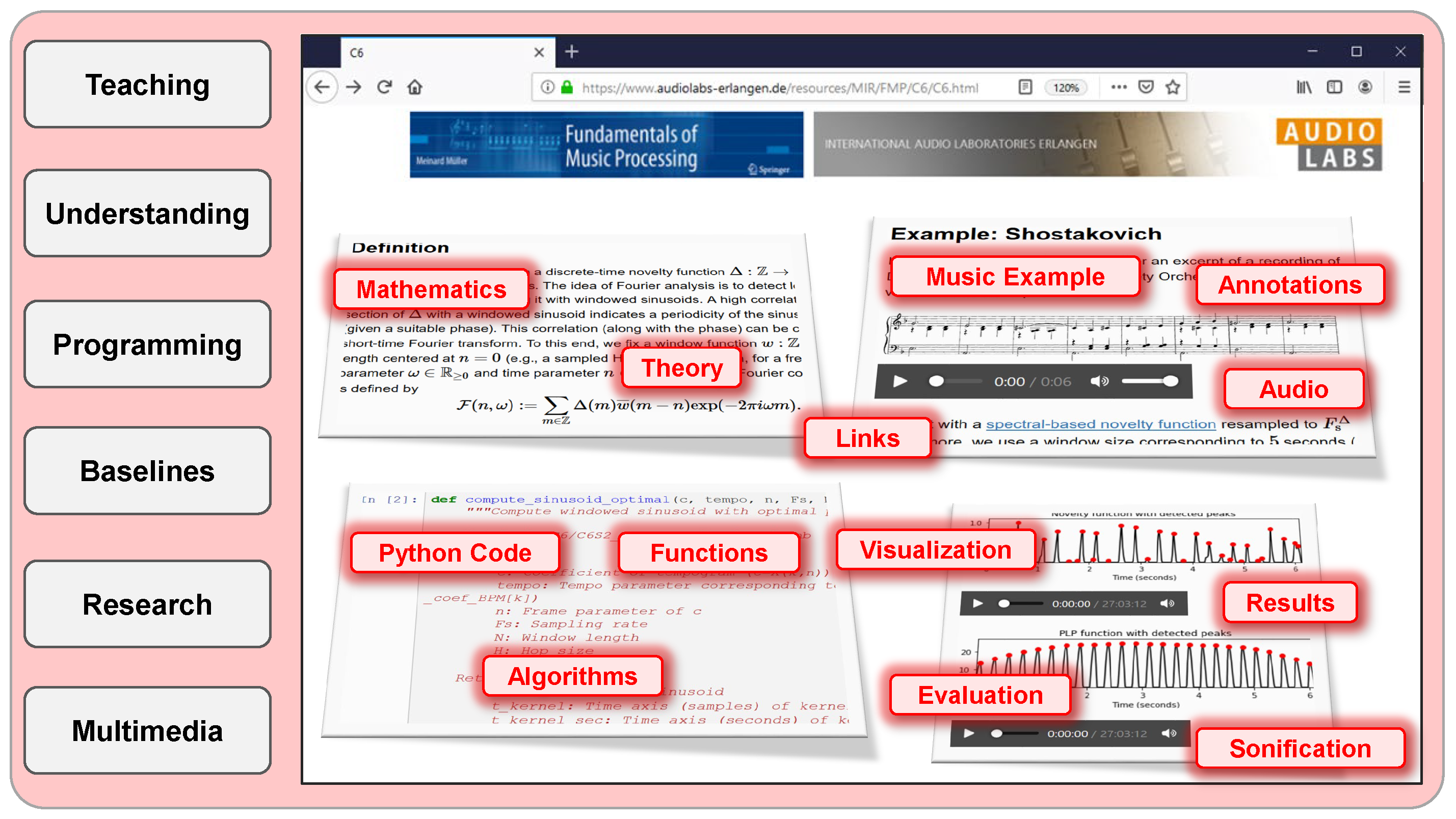
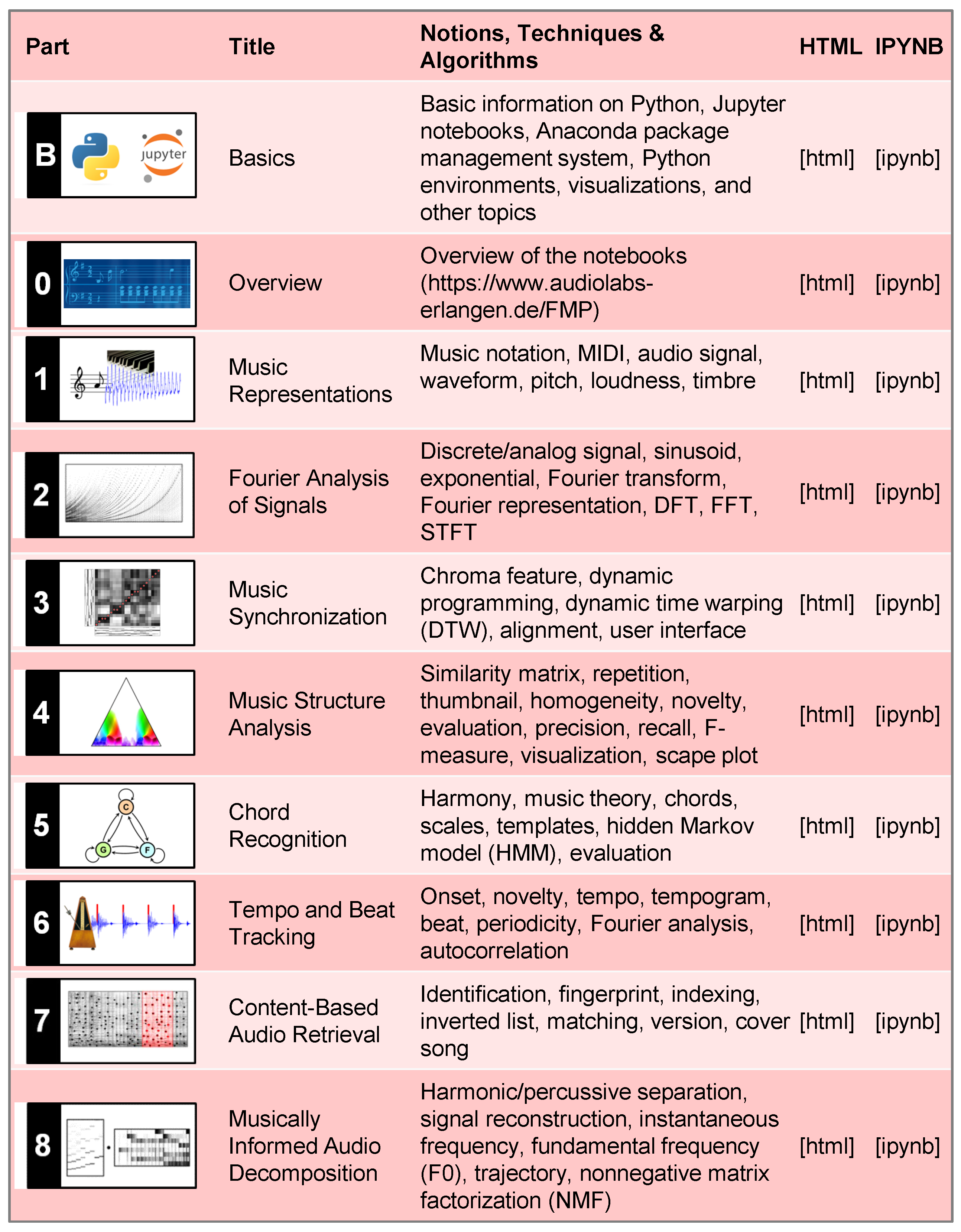
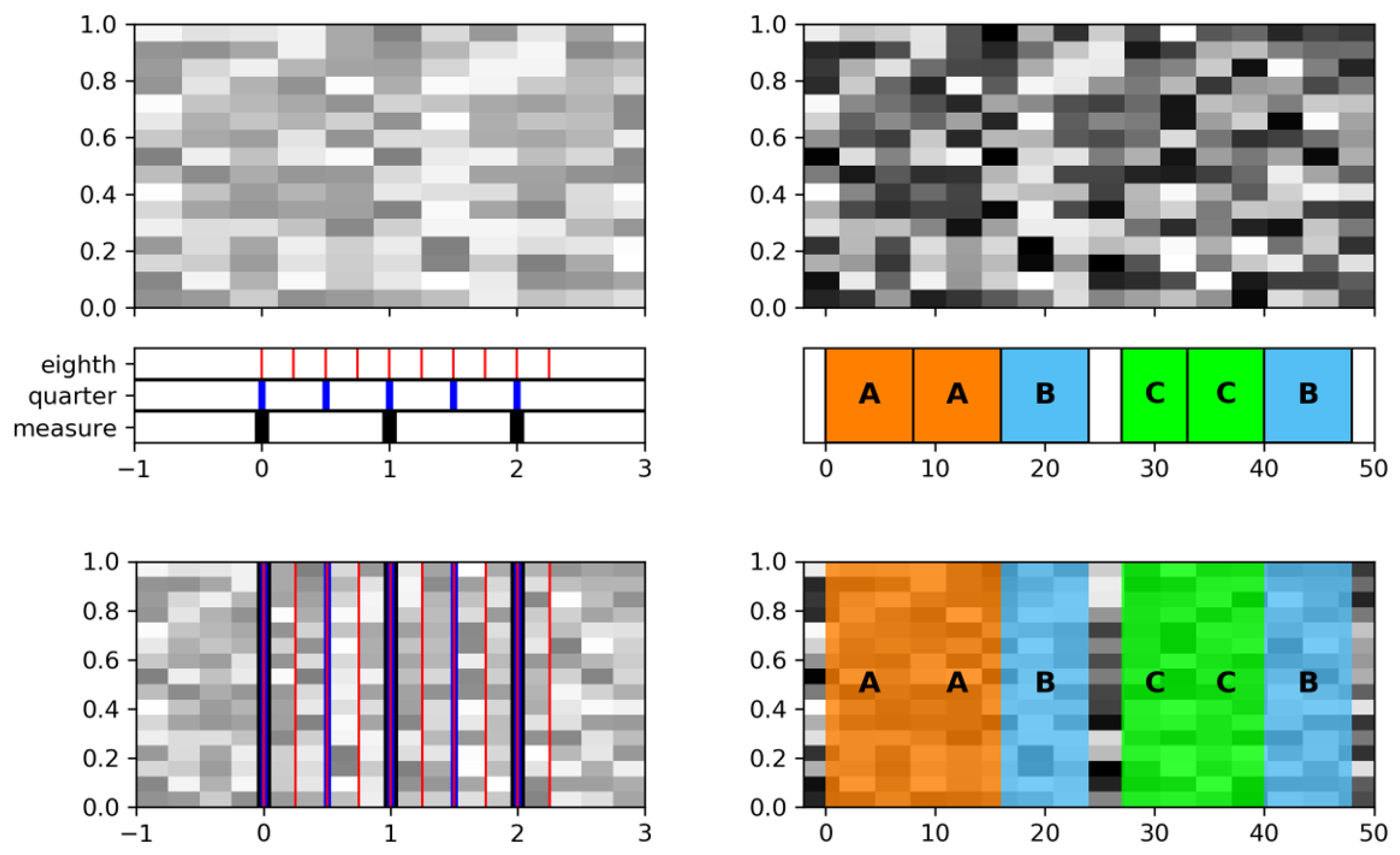
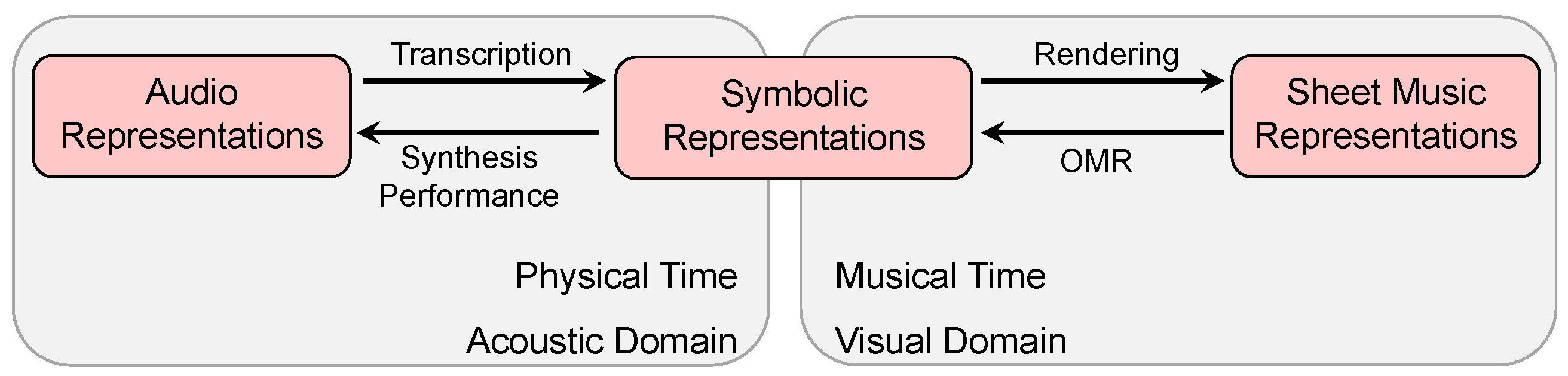
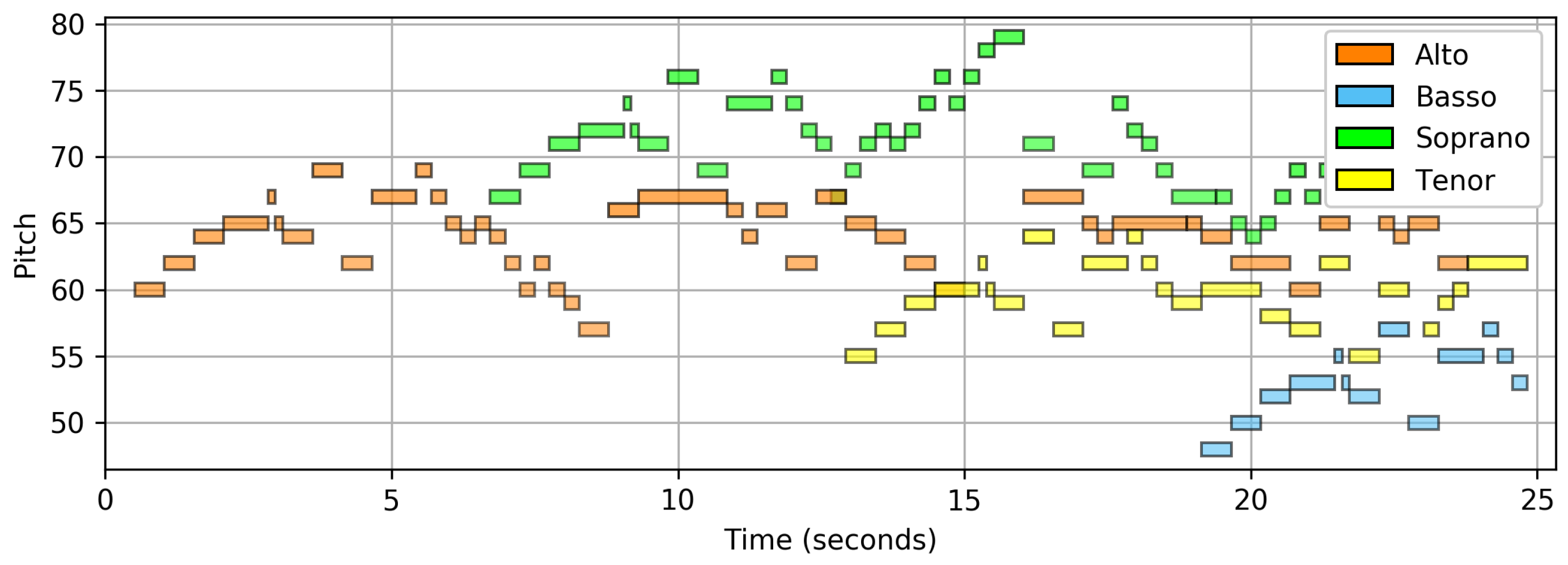
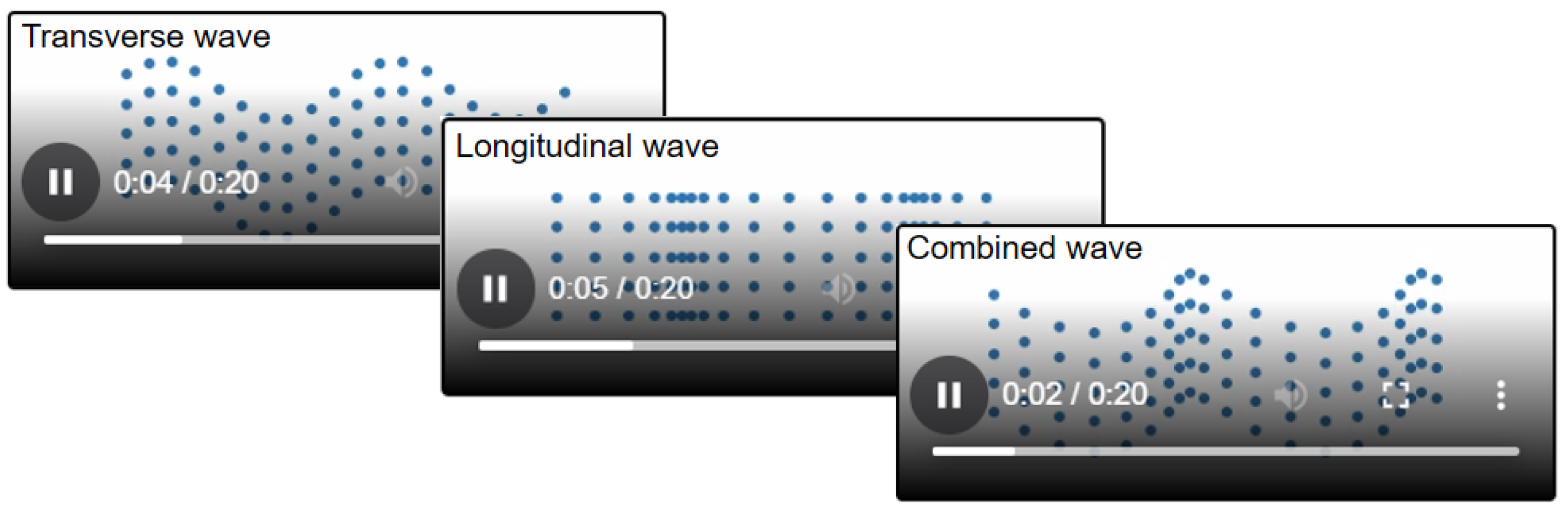
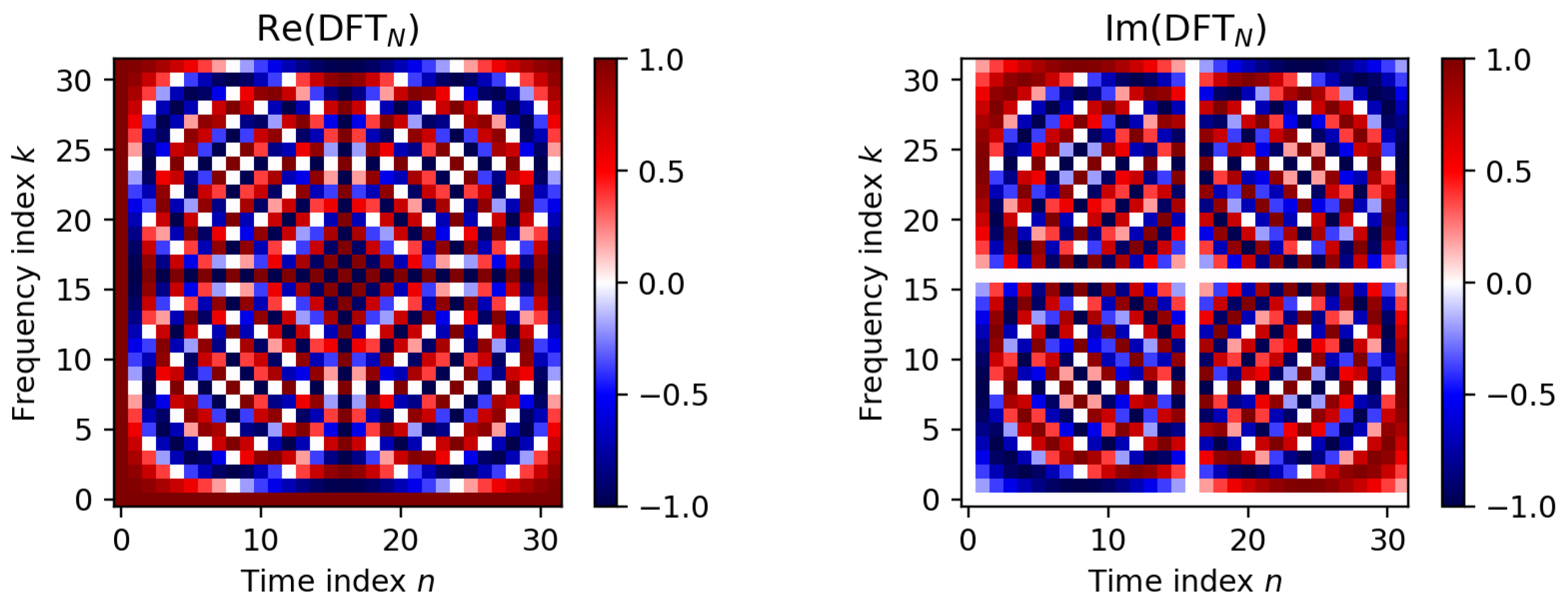
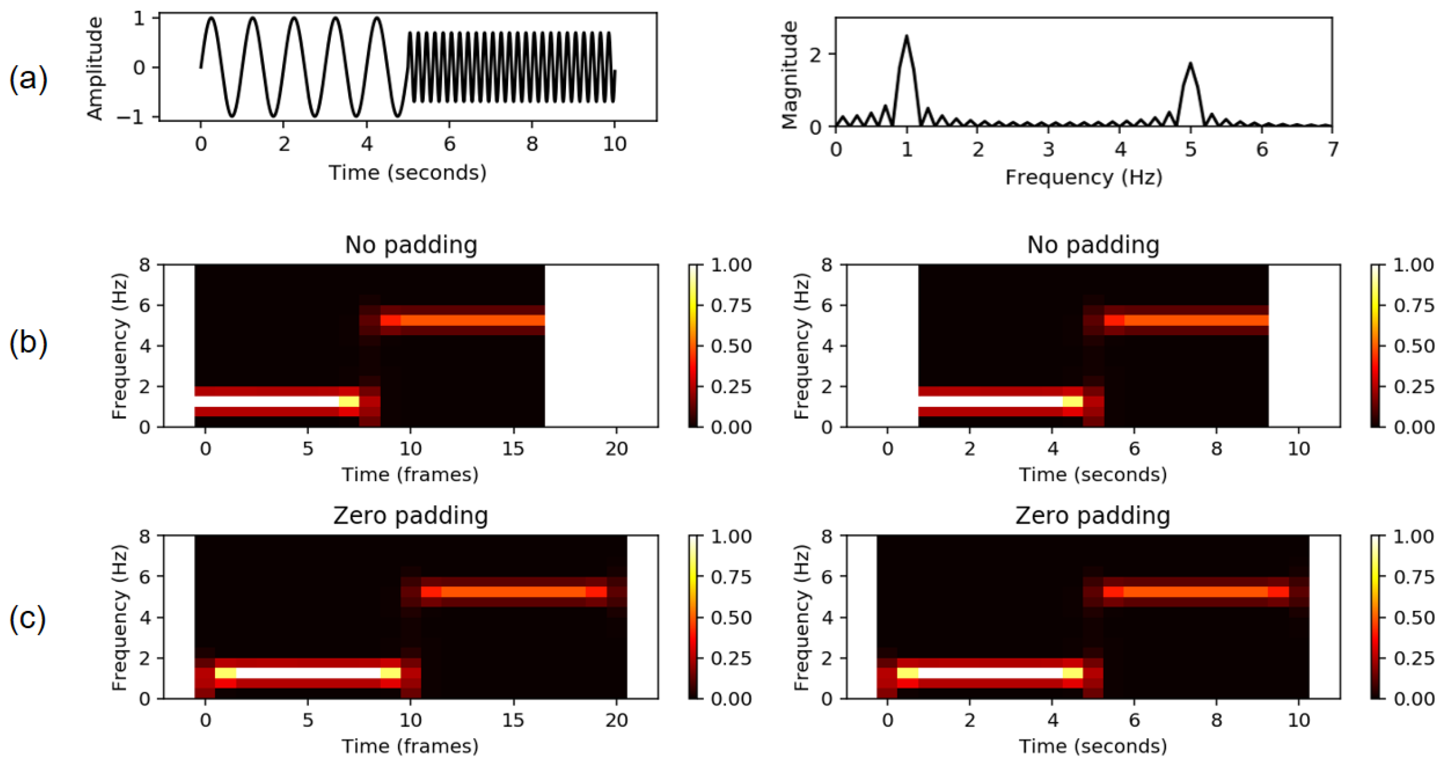
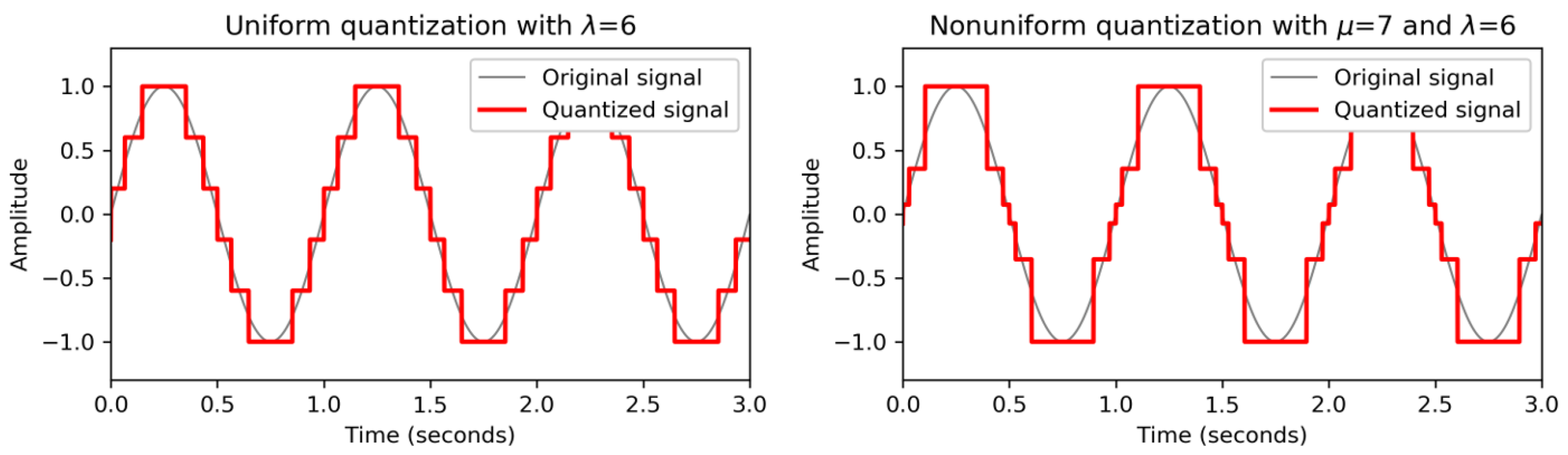
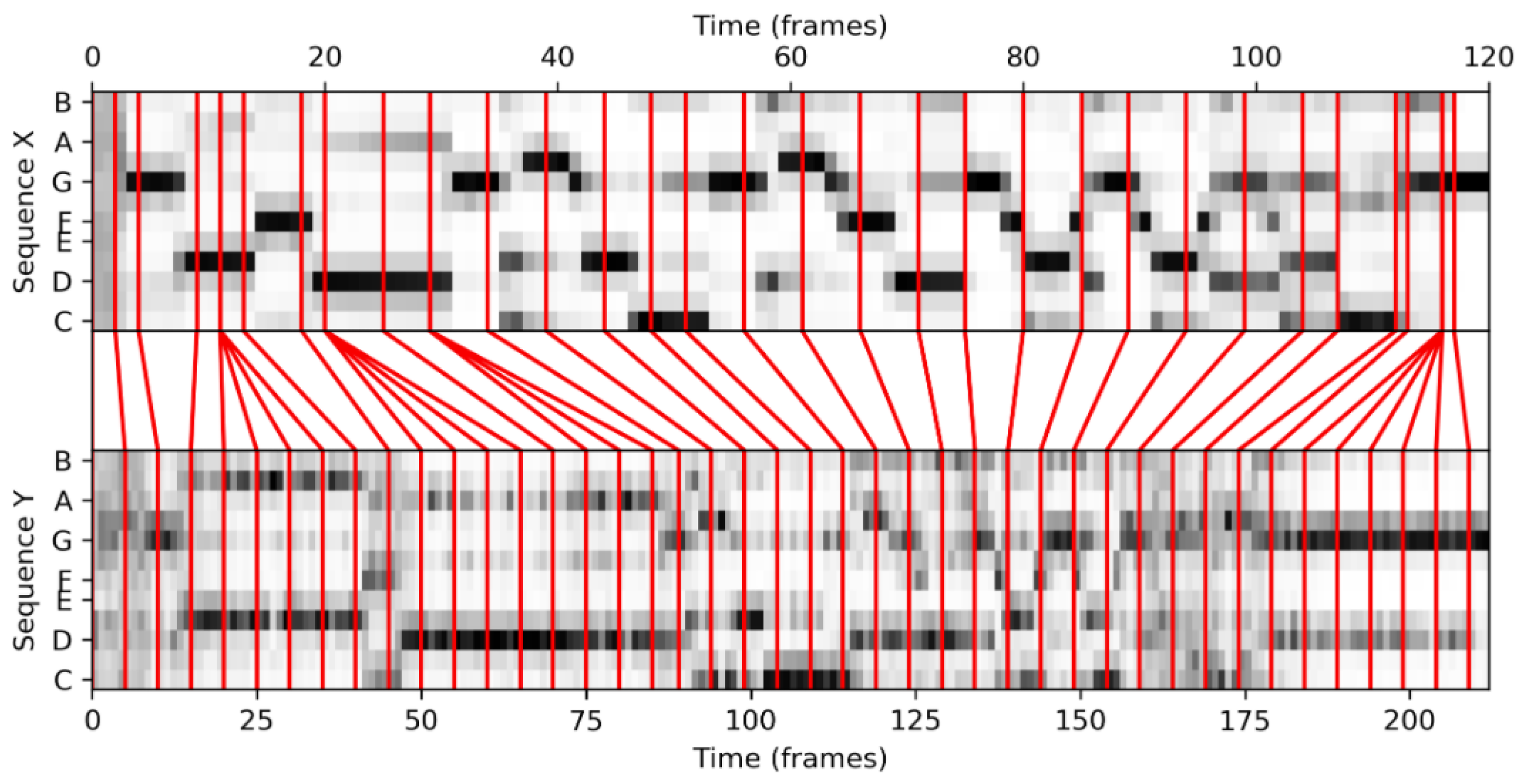
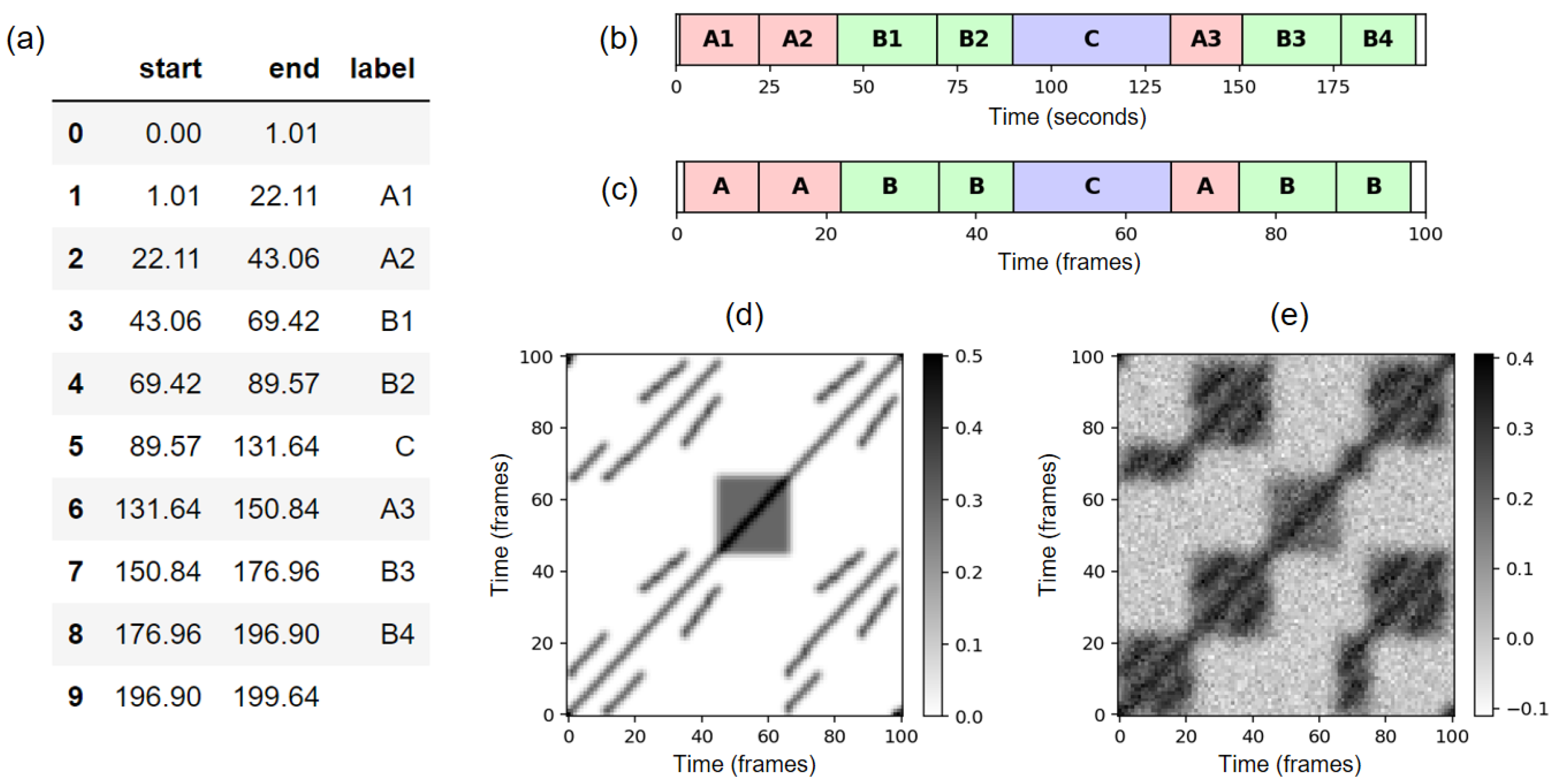
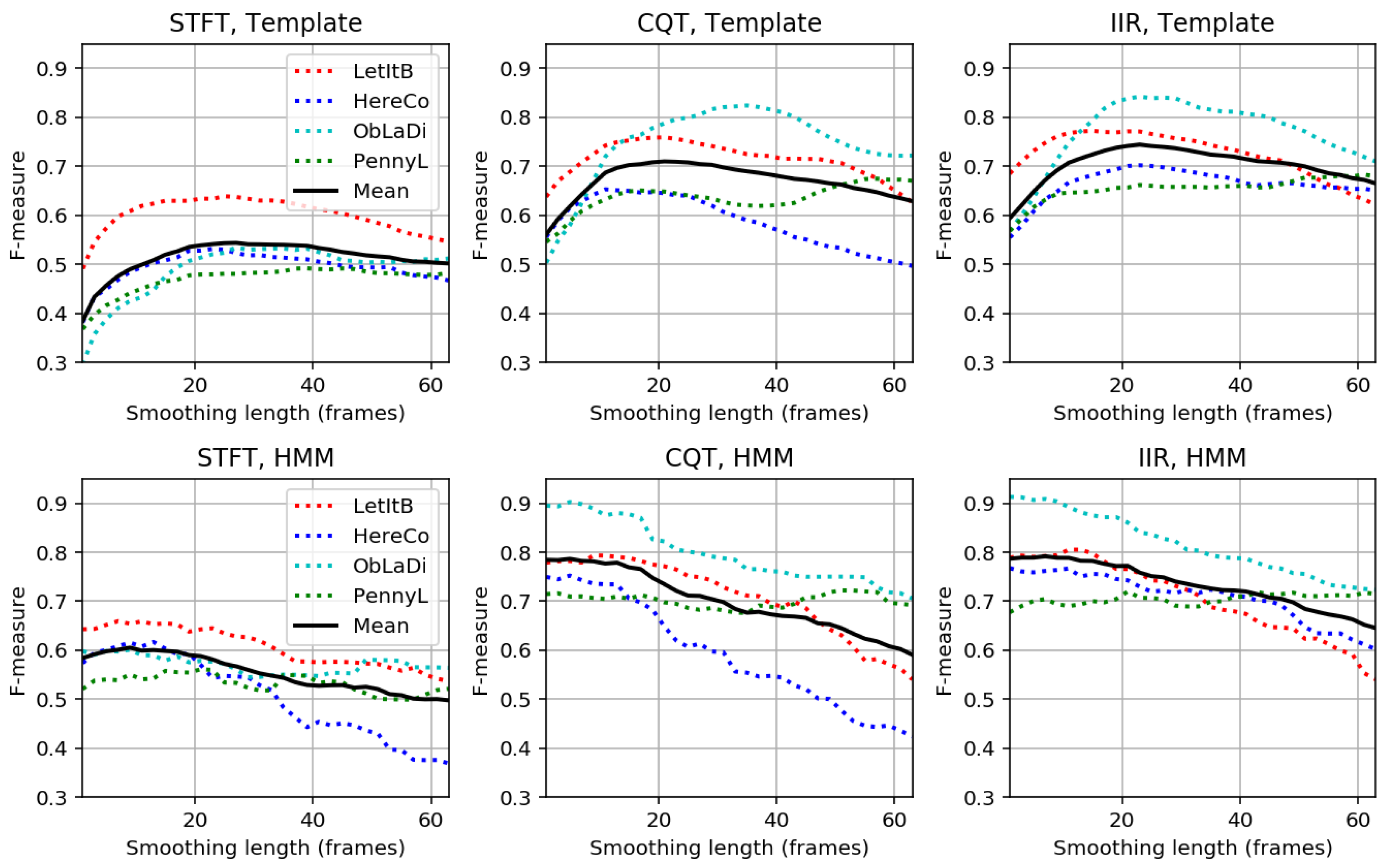
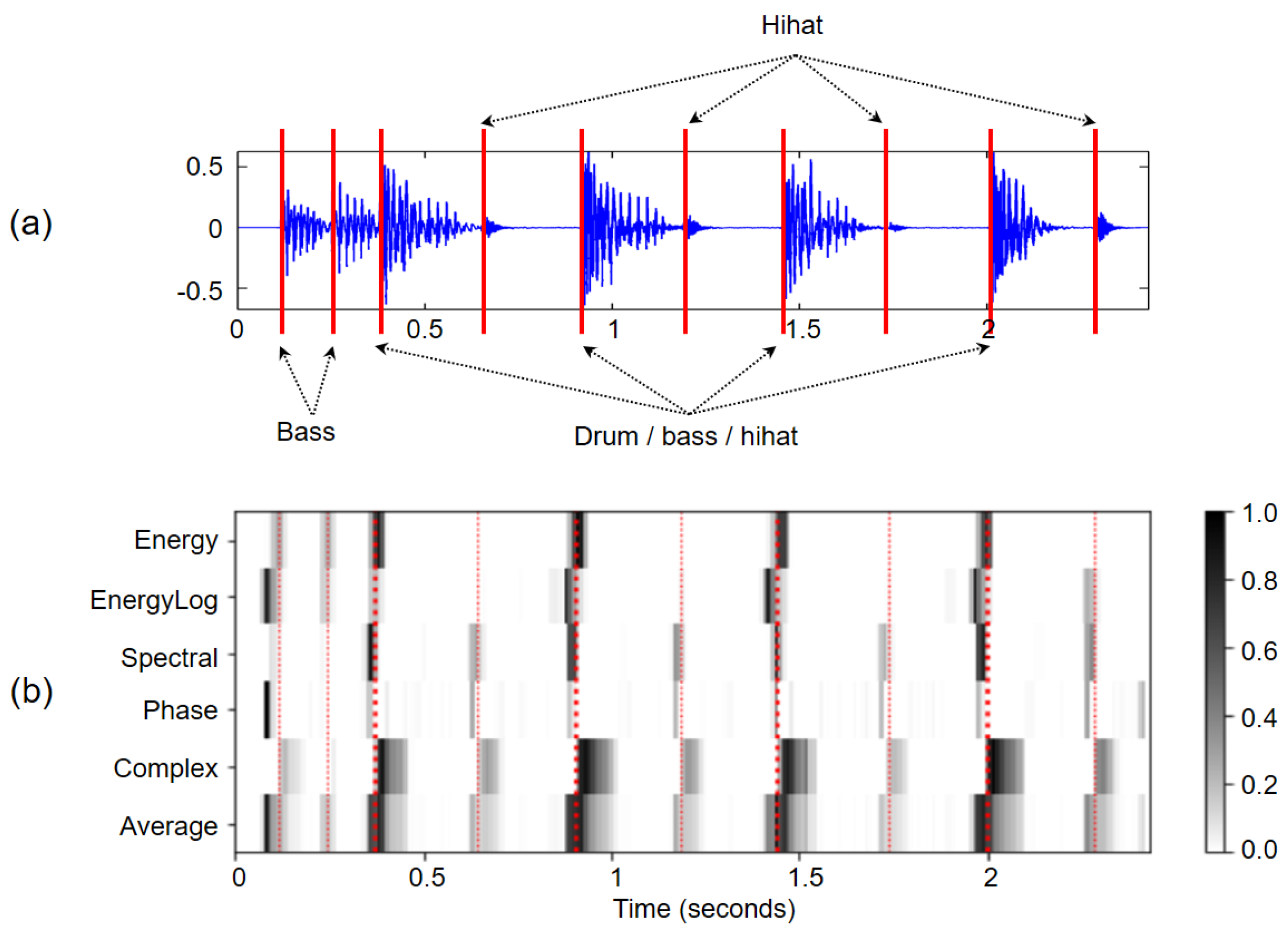
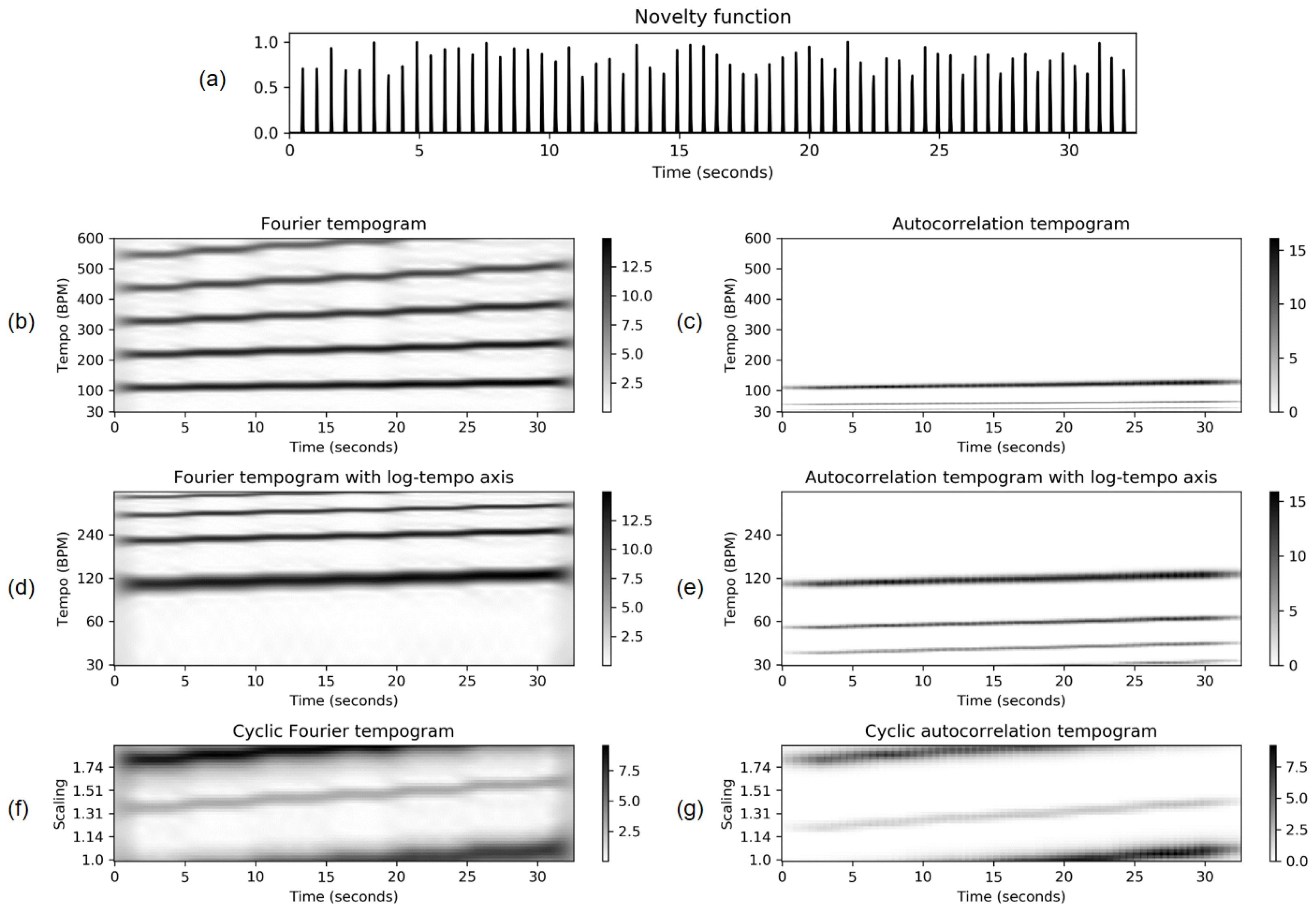
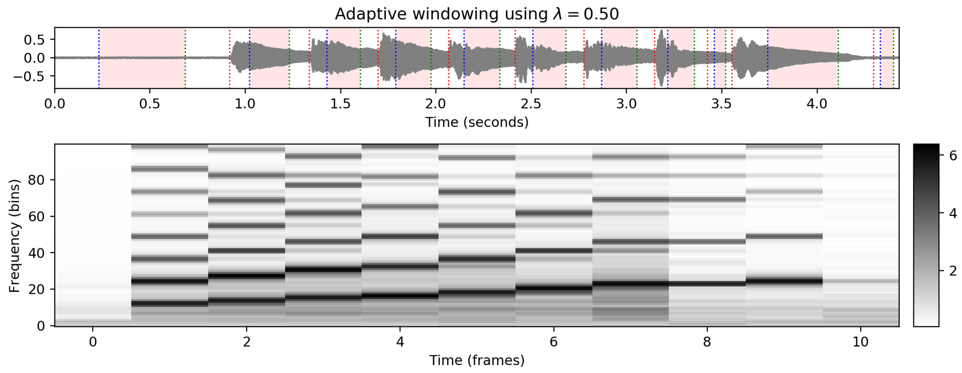
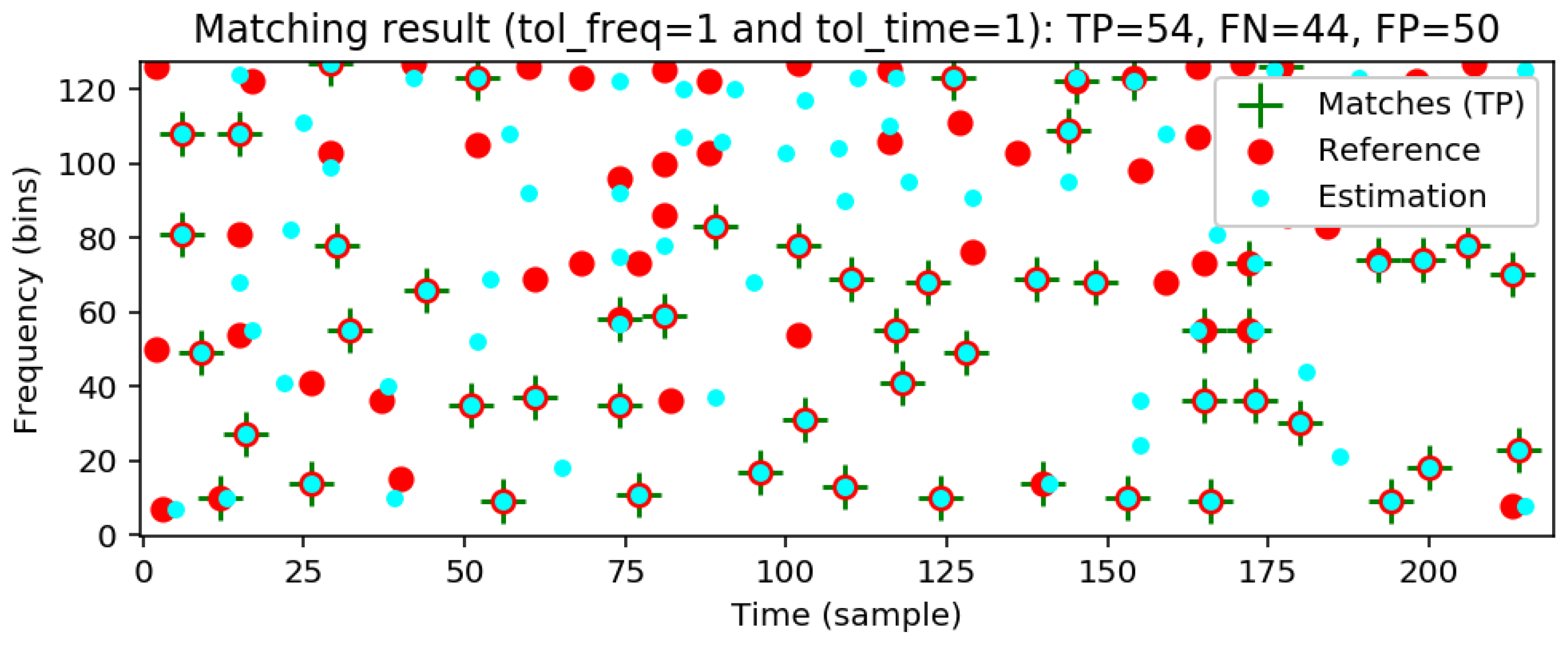
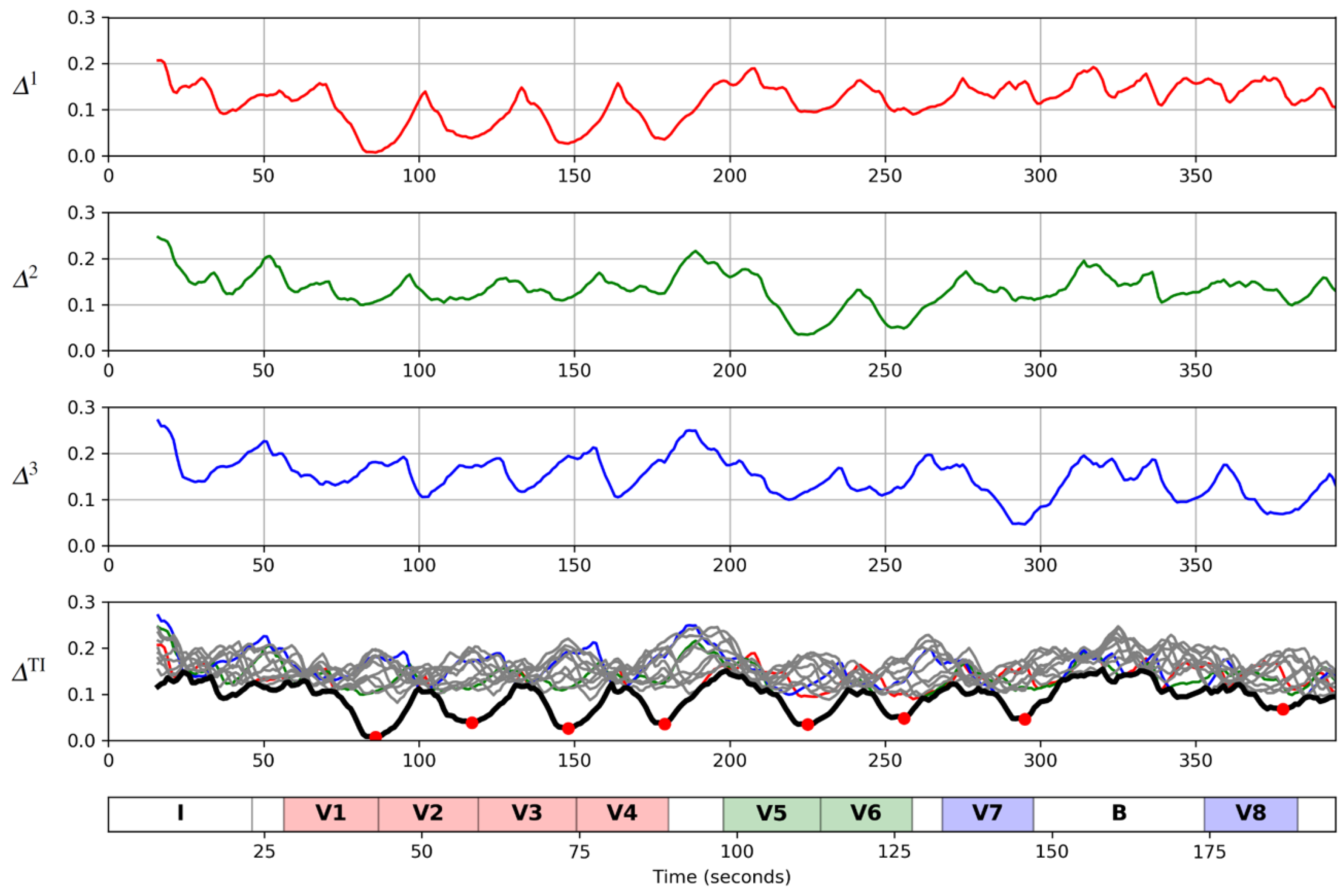
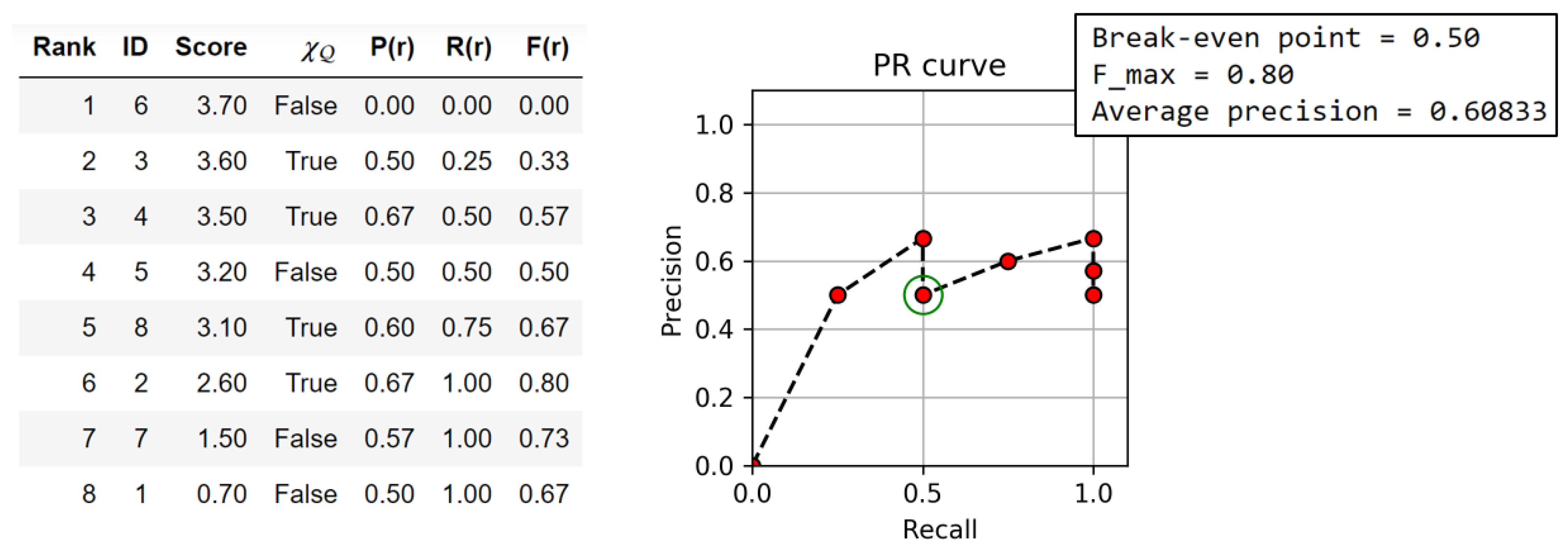
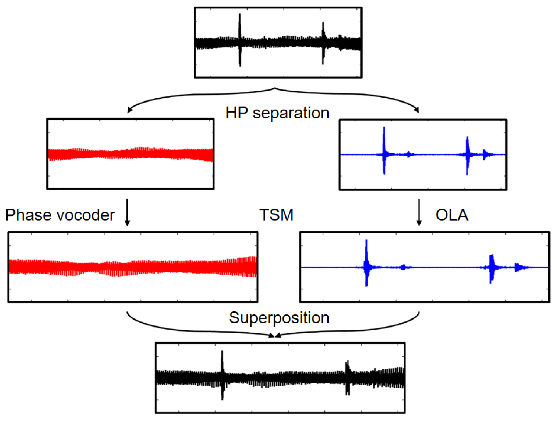
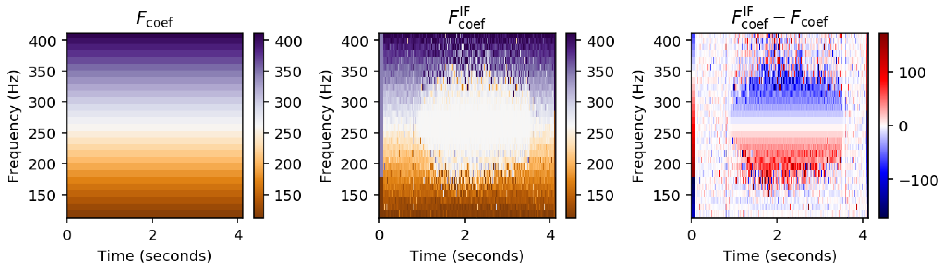
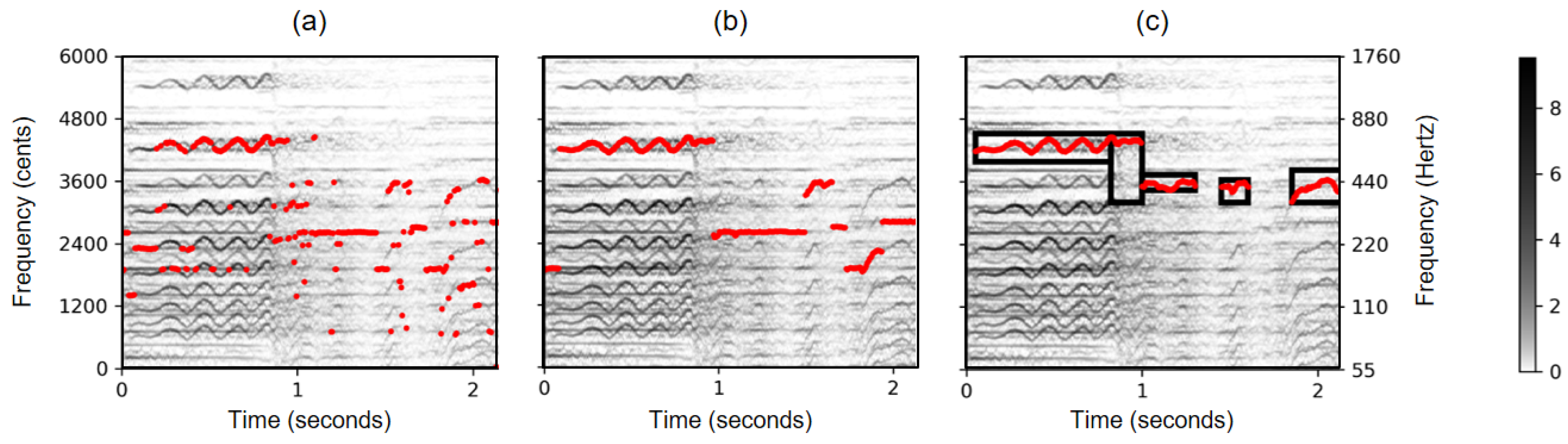
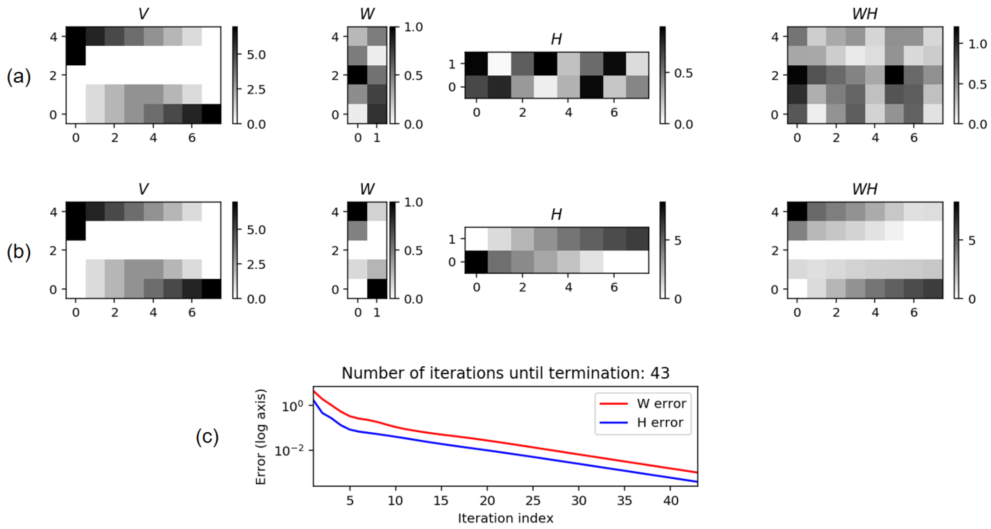
5. Conclusions

In this paper, we provided a guide through the FMP notebooks, which form a collection of educational material for studying central techniques in music processing and music information retrieval. Complementing the textbook [1], the notebooks provide audio-visual material and Python code examples that implement the textbook’s computational approaches, thus bridging the gap between theory and practice. Additionally, the FMP notebooks yield an interactive framework that allows students to experiment with music examples of their own choice, explore the effect of parameter settings, and understand the computed results by suitable visualizations and sonifications. When teaching and learning music processing, it is essential to have a holistic view of the MIR task at hand, the algorithmic approach, and its practical implementation. Looking at all the processing pipeline steps sheds light on the input data and its biases, possible violations of model assumptions, and the shortcoming of quantitative evaluation measures. Only by an interactive examination of all these aspects will students acquire a deeper understanding of the concepts, transitioning from merely understanding concepts to applying them in the context of practical applications.

Besides providing educational material for teaching and learning music processing, the FMP notebooks also comprise a core library of implementations for many previously published MIR methods. Employing and providing Python and Jupyter-based tools, which have been made publicly available for research purposes, the FMP notebooks make a contribution to reproducible research. As emphasized in [59], open source and reproducible research, which comprises both reproducibility (sharing code) and replicability (easily reconstructing a method), are at the core of fundamental research. As such, these topics should be addressed in any curriculum when training advanced students and beginning researchers. In this context, we hope that the FMP notebooks provide an example for best practices.

As in general multimedia processing, many recent advances in music processing have been driven by techniques based on deep learning (DL) [60,61]. For example, DL-based techniques have led to significant improvements for tasks such as music source separation [49,62,63,64], music transcription [65,66], chord recognition [35,67,68,69], melody estimation [70,71], beat tracking [72,73,74], tempo estimation [75,76], version identification [47,48], cross-modal retrieval and alignment tasks [77,78,79], just to name a few. A particular strength of DL-based approaches is their ability to extract complex features directly from raw audio data, which can then be used to make predictions based on hidden structures and relations. Furthermore, powerful software packages (e.g.,  [80]) allow for easily designing, implementing, and experimenting with machine learning algorithms based on deep neural networks. However, music turns out to be a particularly hard domain due to its high complexity and diversity, which requires vast amounts of training data to account for the many different musical and acoustic variations occurring in real-world settings.

Covering the fast-growing and dynamic field of deep learning goes beyond the scope of the FMP notebooks. Instead, the notebooks focus on classical signal and music processing techniques, yielding fundamental insights into the problem at hand and providing explicit baseline approaches one may (and should) compare against when exploring more powerful yet often difficult-to-interpret DL-based learning approaches. Even though being only a small selection of recent DL-based MIR approaches, we hope that the provided references are useful entry points for further reading. Furthermore, we hope that the FMP notebooks yield a sound foundation for students and researchers to transition from classical engineering approaches to the world of deep learning applied to challenging music processing tasks.