Article

Exploiting the Low Doppler Tolerance of Noise Radar to Perform Precise Velocity Measurements on a Short Set of Data

by
Christoph Wasserzier
Fraunhofer Institute for High-Frequency Physics and Radar Techniques FHR, 53343 Wachtberg, Germany
Signals 2021, 2(1), 25-40; https://doi.org/10.3390/signals2010003
Submission received: 1 September 2020 / Revised: 6 October 2020 / Accepted: 6 January 2021 / Published: 21 January 2021
(This article belongs to the Special Issue Signal Processing in Modern Radars)

Abstract

:
The extraction of velocity information from radar data by means of the Doppler effect is the driving factor for the investigations presented in this paper. A method for the quantification of the Doppler tolerance in continuous emission (CE) noise radar is introduced, addressing a current lack in literature within the frame of CE noise radars. It is shown that noise radar is highly sensitive to the Doppler effect, an issue that often results in a low Doppler tolerance especially for long coherent integration intervals. In general, the Doppler sensitivity is considered as a drawback but, in this paper, along with the absence of range-Doppler coupling in noise radar, it is turned into an advantage allowing for a very precise Doppler estimation. This new signal processing approach for Doppler extraction is detailed and its feasibility is proven on the basis of experimental data. The presented method requires much less data, i.e., target illumination time, than conventional Doppler analyses and, therefore, is beneficial in terms of radar resource management.

1. Introduction

The usage of random modulated radar signals was formally described in the year 1959 in [1], often treated as the origin of noise radar technology (NRT). The authors of [2] even trace back the concept of noise radar to an experiment performed in the year 1897. A general introduction and details on noise radar signal processing can be found in [3].
Noise radar technology is well known for its main benefits which are its low probability of intercept (LPI) characteristics [4], its inherent robustness against mutual interference [5,6], and its close-to ideal, thumbtack-like, ambiguity function (AF) [7]. In the latter, neither range nor Doppler ambiguities exist and range-Doppler coupling is absent. This paper adds a new feature to the list of benefits. It is shown that a very precise determination of the velocity of a target may be performed on noise radar data even when the duration of the recording is too short to perform conventional Doppler analyses of the same precision. The work is structured as follows. The introduction continues with background information on conventional Doppler analyses and motivates potential applications for the presented processing scheme. Section 2 defines a formalism to quantify the Doppler tolerance in noise radar, filling a current gap in the scientific literature. The new signal processing scheme for Doppler extraction in noise radar data is presented in Section 3 and applied to experimental data in Section 4 and Section 5. Finally, a discussion of the achievements is given in Section 6.
The investigation presented in this paper is a follow-on research based on the findings of [8], a PhD thesis completed during doctoral studies at the University Tor Vergata of Rome, Italy, in cooperation with the German research institute Fraunhofer FHR.

1.1. Background

Radar signals are sensitive to the motion of the target and to the motion of the radar platform itself. The Doppler effect causes a frequency shift of the involved radio waves in dependency of the relative radial velocity v r between the radar and the target. In many radar applications, the Doppler frequency f D ( t ) is assumed to be constant during the observation time and is approximated, neglecting relativistic effects, by
f D = 2 v r f 0 c ,
with f 0 denoting the carrier frequency of the radar signal.
The historical principle [9] to compensate for the Doppler shift of a radar echo uses a Doppler filter bank, that is, a bank of matched filters which are often tuned to equally spaced Doppler frequencies. In this early implementation, the matched filtered signals then were delivered to a decision network, which in [9] is a “greatestof” signal selection. The Doppler filter bank principle was improved over the years leading to sophisticated designs such as [10]. Digital signal processing has opened many occasions for strategies of Doppler analyses, used for the extraction of a target’s velocity information, and also for Doppler compensations.
To efficiently implement a digital Doppler filter bank, a Fast Fourier Transform (FFT) is applied to a series of range measurements. A detailed description can be found in ([11], [ch.17]). The number of consecutive range measurements shall be denoted by P which, together with the pulse repetition interval T P R I of a conventional radar, forms the coherent processing interval of the FFT being T C P I = P · T P R I . The digital sampling rate of the resulting FFT is equal to the pulse repetition frequency PRF = 1 T P R I . This signal domain, which represents temporal variations of range measurements, is often referred to as the slow-time scale [12]. A general design criterion of Doppler filters is given in ([13], [ch.18]), stating that the bandwidth of each Doppler filter needs to span at least the frequency distance of the filters, a condition which is inherently met when the FFT is applied. The frequency resolution of the Doppler-FFT corresponds to the inverse of the coherent processing interval equal to
Δ f D = 1 P · T P R I .
Moreover, the measurement of the Doppler frequency is ambiguous by multiples of the PRF [14], unaffected by the value of P.
In order to apply the method of Doppler filter banks to continuous radar signals, either for deterministic continuous wave (CW) radars like the well-known frequency modulated continuous wave (FMCW) or for CE noise radar, a functional equivalent to the PRI needs to be identified. For continuous radar signals, having a duty cycle of 100%, obviously, no pulses exist but the Doppler filter bank principle is directly applicable by segmenting the radar signal properly into slices of duration T r . The choice of T r depends on the waveform modulation. In an FMCW signal, for example, the segmentation ought to follow the periodic modulation: it practically covers a single frequency ramp in order to maintain the full signal bandwidth during each range measurement. But for the non-repetitive signals in continuous emission noise radar, the segment duration T r can be chosen freely: The continuous emission of noise radar is understood as an interruption-free non-repetitive modulation based on a random process of limited, constant bandwidth. The randomness of this modulation is non-repetitive and the full signal bandwidth B is covered in any segment T r that satisfies the requirement B · T r 1 .
Consequently, in continuous emission radars, the interval T C P I of an FFT-based Doppler analysis may be formed by P segments, each of duration T r .

1.2. Motivation

The relationships described in Section 1.1 indicate some important radar design criteria in the context of the extraction of velocity information from radar data:
1.
Precise Doppler measurements require long coherent integration intervals, see (2)
2.
The higher the center frequency of the radar emission, the higher is the Doppler shift for a given radial velocity v r , see (1)
3.
The higher the center frequency, the shorter is the required coherent integration interval for a given precision Δ v r of the velocity measurement
For these considerations, many Doppler radars operate at center frequencies of 10 GHz and above. As an example, the commercial Doppler radars of the company Blighter, used for ground surveillance and drone detection, operate in the Ku-band around 16 GHz [15]. These high frequencies are usually applicable for short-range and medium-range applications. Common long-range radars, instead, operate in lower frequency bands such as marine navigation radars that transmit mostly S-band signals.
The following example illustrates the problems of accurate Doppler measurements with such a navigation radar set. The aimed velocity estimation shall be set to an accuracy of 1 knots, that is, Δ v r = 0.514 m/s, for a hypothetical S-band radar operating at a center frequency of f 0 = 3 GHz. From (1) results that the Doppler precision should not exceed a value of Δ f D = 2 Δ v r f 0 c = 10.28 Hz. This increment, according to (2), defines the minimum coherent processing interval to T C P I = 1 Δ f D 100 ms. But a strong discrepancy occurs when the minimum required value of T C P I is compared to the typical design of long-range navigation radars such as the JMR-5472-S [16]. With a typical beam width of θ = 2 degrees and a rotation of the antenna at ω = 24 revolutions per minute, a maximum time-on-target of about 14 ms is achieved by such a radar set. This interval is much shorter than the minimum coherent processing interval required for the respective Doppler analysis. But the method presented later in this paper might solve this issue. The duration of the experimental data of Section 4, deliberately limited to 12 ms, was chosen in agreement with the just made considerations.
Moreover, the Doppler extraction method presented in this paper is also considered as beneficial for modern agile multi-role radars that perform different tasks, enabled by a sophisticated resource management. One important resource is the illumination time, that is, the interval at which the antenna (which usually is a phased array antenna) of the multi-role radar is locked to a specific direction. The Doppler extraction procedure presented in this paper reduces the required time-on-target by a waveform-specific signal processing algorithm making use of the characteristic Doppler tolerance of a continuous emission noise radar. This is particularly important for phased array radar tracking applications [17] which involve rapidly switched beam positions and demand for an efficient management of the revisit time and the time-on-target. The resource management becomes even harder when it comes to multi-function RF systems (MFRFS) that combine radar, electronic warfare and communication tasks by a single sensor [18]. A general concept, of how these MFRFS might further benefit from the use of noise radar technology was presented in [19].

2. Quantification of the Doppler Tolerance in CE Noise Radar

The general problem of Doppler tolerance in radar is discussed in the literature with different terminology. In 1966, the author of [20] aimed for a waveform design with Doppler invariance by focusing on range-Doppler coupling. As the latter is absent in random waveforms, the approach presented in that paper is not applicable to noise radar technology. The problem of Doppler tolerance is also discussed in [21,22,23], but the focus of these papers lies on transmitter code-design which contradicts the idea of randomness in noise radar emissions. The authors of [24,25] propose a combination of transmission wave design (Golay) combined with expensive phase compensations on receive. An idea, rejected for the same reason. Also in [26], the achievement of Doppler invariance is used as the design criterion for specialized codes, still, that paper does not formally investigate the Doppler tolerance.
The most formal approach to Doppler tolerance of radar waveforms can be found in [27] biased by an LFM signal background. But many aspects in [27] can be easily ignored when focusing on noise radar: The particular shape of the ambiguity function of noise signals and the absence of range-Doppler coupling in noise radar allows for a description of the AF by two cuts [7], one cut along the delay axis and a second cut along the Doppler axis.
In [28], the Doppler tolerance of OFDM radar waveforms is formulated as a function of the number of carriers in the OFDM signal. The results are not directly applicable to CE noise radar but the paper formulates a general definition of a Doppler characterization by defining a loss-measure based on the ambiguity function. This approach inspired the, still different, procedure for characterizing the Doppler tolerance in CE noise radar of the current paper.
The ambiguity function [29], more precisely the auto-ambiguity function, of a radar waveform u ( t ) shall be denoted as
χ ( τ , f D ) = u ( t ) u * ( t τ ) e j 2 π f D t d t ,
which defines a two-dimensional function in the delay-Doppler coordinate system. The ambiguity function for f D = 0 forms the auto-correlation function (ACF) of the signal u ( t ) with
R u u ( τ ) = u ( t ) u * ( t τ ) d t .
Any concentration of energy located aside the origin of the delay-Doppler coordinate system in (3) might cause ambiguous range-Doppler measurements in radar applications. This might potentially result in the extraction of wrong target parameters or even in false targets. But CE noise radar has an ambiguity function which is close to ideal as is shown in Figure 1 representing an illustration of the thumbtack-shaped ambiguity function of an idealized noise waveform.
In real-world applications, restricted to the usage of band-limited and finite noise signals, the resulting ambiguity function still remains similar to the idealized AF shown in Figure 1 but it does not form a two-dimensional Dirac function (also known as Kronecker Delta). Instead, the single peak in the origin of the delay-Doppler coordinate system has a certain spread in both dimensions and is of finite height. The peak height, characterised by the peak-to-average-sidelobe ratio, is determined by the time-bandwidth product of the waveform [30]. The spread of the peak in the delay dimension defines the well-known range resolution and is caused by the finite signal bandwidth ([31], [ch.9]). However, the spread in the Doppler dimension, along with its cause, is evaluated here in order to extract a measure for the Doppler tolerance of noise radar technology.
The matched filter output of a radar echo shows a particular signal-to-noise ratio (SNR), evaluated by common detection algorithms as presented in ([32], [ch.2]). It is
SNR = P y P N ,
where P y denotes the signal power of the, in the frame of this paper matched filtered, radar echo and P N denotes the power of the receiver noise, bounded below by the thermal noise.
The current paper proposes a quantification of the Doppler tolerance of CE noise radar by investigating the influence of the Doppler effect on the matched filtered signal power P y . In this approach, the squared ambiguity function | χ ( τ , f D ) | 2 , directly proportional to P y , is used as the main indicator of the loss that a particular Doppler shift of an echo signal has on the resulting correlator output. As the current work focuses on CE noise radars, the following derivations make use of the characteristic thumbtack-like shape of its ambiguity function. These considerations lead to a loss function L ( τ , f D ) , given by
1 L ( τ , f D ) = χ ( τ , f D ) 2 χ ( 0 , 0 ) 2 ,
with the maximum value of the ambiguity function always located at ( τ = 0 , f D = 0 ) .
The illustration of the ambiguity function in Figure 1 emphasizes the absence of range-Doppler coupling in noise radar [7] why, in this case, (3) may be computed by
χ ( τ , f D ) = χ ( τ , 0 ) · χ ( 0 , f D ) .
This independence of delay and Doppler in the ambiguity function of CE noise radar leads to the idea to fully characterize this Doppler tolerance by evaluating the zero-Delay cut (ZDC) of the AF, that is, χ ( 0 , f D ) .
Consequently, for CE noise radar, the indicator of the Doppler tolerance, defined in (6), simplifies to
1 L ( f D ) = χ ( 0 , f D ) 2 χ ( 0 , 0 ) 2 .
A threshold value of L t h = 2 is set that represents the “3 dB point” of the ambiguity function in the Doppler dimension. Consequently, a cutoff-frequency f 3 d B shall be defined as
f 3 d B = m i n ( | f D | ) : L ( f D ) L t h .
In the following, the cutoff-frequency is investigated by evaluating the respective zero-delay cut of the ambiguity function depending on the matched filter duration.
In noise radar technology, the emitted signal g 0 ( t ) is often assumed to be the realization of a Gaussian or at least of an ergodic random process. The echo of a target located in a particular distance D and moving with a radial velocity v r forms a received signal
s 0 ( t ) = A · g 0 t 2 D c e j 2 π f D t ,
which is a delayed and Doppler-shifted copy of the transmitted signal g 0 ( t ) attenuated by a factor A that mainly depends on the range and the size of the target. The term f D was defined in (1). A range measurement can be performed by computing the cross-correlation of the received signal and the transmitted signal, in other words by a matched filter process. But any practical computation of the matched filter has a finite duration which requires a segmentation of the continuous noise signals s 0 ( t ) and g 0 ( t ) to finite signals s ( t ) and g ( t ) .
In general, the segmentation procedure of a noise radar waveform can be modelled by an appropriate window function w ( t ) from which a signal,
u ( t ) = n ( t ) · w ( t ) ,
is computed with n ( t ) representing a realization of a white Gaussian process filtered to a 3 dB bandwidth equal to B. A specific window function is presented later in this section.
From the definition of the ambiguity function, given in (3), it follows that for τ = 0 the phase of the waveform u ( t ) has no influence on the zero-delay cut χ ( 0 , f D ) . The relationship of the waveform u ( t ) on the ZDC of the coherent AF can be expressed in compact form [14] by
χ ( 0 , f D ) = F u ( t ) 2 ,
with F · denoting the Fourier transform ([33], [ch.2]), which for a signal x ( t ) is
F x ( t ) = X ( f ) = x ( t ) e j 2 π f t d t .
From (11) and (12) follows that the zero-delay cut of the resulting ambiguity function of u ( t ) is computed by a convolution (the symbol is: * ) to
χ ( 0 , f D ) = F n ( t ) 2 * F w t 2 , as w ( t ) 0 t .
For B T 1 , the convolution in (14) may be approximated by
χ ( 0 , f D ) R n n ( 0 ) · F w t 2 .
A detailed derivation of this approximation can be found in [34]. Equation (15) indicates that the Doppler tolerance in noise radar is mainly influenced by the shape of the window function w ( t ) and quantified as follows.
For a simple segmentation of the waveform n ( t ) into slices of duration T 0 , a rectangular window,
w r t T 0 = 1 , for t T 0 2 0 , otherwise ,
is implicitly applied by the segmentation procedure leading to a signal
u r ( t ) = n ( t ) · w r t T 0 ,
for which the Doppler tolerance is computed in this section. Figure 2 illustrates the signal model of u r ( t ) , created from a noise source N 0 that, idealized, is assumed to have a Gaussian distribution.
For a rectangular window function, as defined in (16), it is w r ( t ) d t = T 0 and, thus, the resulting gain of the respective matched filter process is equal to
G M F , r = 1 L r ( f D ) B T 0 ,
with B denoting the bandwidth of the signal n ( t ) .
The equation stated in (15) stresses out that the Doppler behaviour of the ambiguity function of the particular noise waveform defined in (11) is dominated by the shape of the window function w ( t ) . The normalization in (8) and the fact that R n n ( 0 ) = c o n s t . in (15) lead to the following formulation of the Doppler-sensitive loss function of the signal u r ( t ) . It is
1 L r ( f D ) = F w r t T 0 2 = sin ( π f D T 0 ) π f D T 0 ,
where T 0 represents the duration of the rectangular window, defined in (16). This Doppler-behaviour is illustrated in Figure 3.
Equation (19) describes a symmetrical function and, thus, only the positive Doppler axis is drawn in Figure 3. The dotted red line indicates the position of the cutoff Doppler frequency, achieved by applying the rule of (9) to (19) and resulting in
| f 3 d B , r | 0.443 T 0 .
The subscript r indicates the relationship of this Doppler tolerance rule to the particular shape of the rectangular window function of the noise signal u r ( t ) as defined in (16) and (17).

Impact on Noise Radar Implementations

The interpretation of (20) leads to the general statement that the longer the matched filter duration T 0 the narrower is the main peak of the function 1 / L r ( f D ) , as f 3 d B 0 for T 0 . Therefore, all noise radar applications that use long signal segments for the range-correlation have to cope with a resulting limited Doppler tolerance illustrated by the following example.
An X-band radar is considered whose parameters are roughly compliant with the demonstrator used in Section 4 and comparable to small marine navigation radars such as [35]. The radar emission is assumed to be restricted, for example by regulations or hardware limitations, to a bandwidth of 50 MHz around a center frequency of 10 GHz. Thus, for an LPI application, any reduction of the emitted power whilst maintaining a certain aimed signal-to-noise ratio for a given task can only be accomplished by utilizing a long processing interval. For example, a radar pulse of 1 μ s duration and 1 kW peak power might be replaced by a noise signal of the same bandwidth but with 1 W peak power and 1 ms duration. Without going into the details of any actual radar task, a coherent processing interval of T r = 1 ms shall be considered favourable for the noise radar in this paragraph leading to a maximum coherent processing gain of G = B T r 47 dB. According to (20), this value of T r would result in a Doppler cutoff frequency of f 3 d B = 443 Hz.
Table 1 illustrates the Doppler tolerance of this particular radar implementation with respect to common radar targets moving at typical velocities. The slowest target, a sailing boat given in the first line of Table 1, is the only target that is compliant with the Doppler tolerance requirement of f D < f 3 d B . For all the other targets, either a cost-intense Doppler compensation needs to be performed or the coherent processing interval, that is, the segment duration, needs to be shortened to a value T r T ^ 0 , presented in the last column of the table, with the consequence of a reduced achievable processing gain. The duration T ^ 0 0.443 f 3 d B , derived from (20), is interpreted as the Doppler-tolerant segment duration.
However, for many applications, especially with LPI background, the coherent processing interval needs to have a certain duration according to the requirements on the processing gain. If the maximum expected Doppler frequency exceeds the f 3 d B , then a computationally intense Doppler compensation becomes essential in noise radar even in cases at which the extraction of the target velocity is not required.
This fact might be considered as a drawback of noise radars but for those applications that indeed ask for Doppler information of the targets, the Doppler sensitivity of noise radar provides an advantageous opportunity that is presented in the next sections including a set-up of two road vehicles for an experimental proof of this idea.

3. Signal Processing Method for a Precise Velocity Extraction

This section presents a processing scheme utilizing the Doppler sensitivity, the absence of range-Doppler coupling in noise radar and the fact that for B T 0 1 the signal bandwidth B of a (pseudo-)random signal is not affected by the segment duration T 0 . This method reads the functional relationship of (19) in a different light. The deep nulls of the sinc-shaped Doppler-dependency allow for a precise evaluation of the Doppler frequency as the zero points of this function occur at positions for which
f D T 0 = n , n N +
holds true. In Section 2, T 0 was considered as a fixed value and (19) was computed for different values of f D in order to characterize the Doppler tolerance of a given matched filter implementation in noise radar.
The idea, here, is to find an unknown Doppler frequency by evaluating the output of multiple matched filter processes, each having a different duration T, that are applied to an identical set of data. However, a variation of the matched filter length also influences the processing gain (18) where 1 L ( f D ) has to be evaluated. In noise radars, the bandwidth B is constant in all those segments of reasonable duration, as discussed above. Thus, it is only the variation in the matched filter duration which has to be compensated for. This implies the appropriately normalized function
R s g ( τ D ) ( T ) = 1 T T / 2 T / 2 s ( t ) g * ( t τ D ) d t .
Equation (22) describes the matched filter procedure of a signal s ( t ) with the replica signal g ( t ) for a single delay value τ D but different matched filter durations T. The delay value τ D = 2 D c corresponds to the distance D of a previously detected target whose velocity information shall be extracted. The term c denotes the speed of light.
But a major difference between the functions of (22) and (19) exists for small input values. When f D 0 , the relation of (19) converges to unity, whereas for T 0 the relation of (22) converges to zero. For this reason, the method of Doppler frequency extraction evaluates the distance between subsequent zero points from which the Doppler frequency of the target can be extracted as follows. For any two subsequent zero points with indices n and ( n + 1 ) it is
Δ T = ( n + 1 ) 1 f D n 1 f D = 1 f D
and therefore,
f D = 1 Δ T .
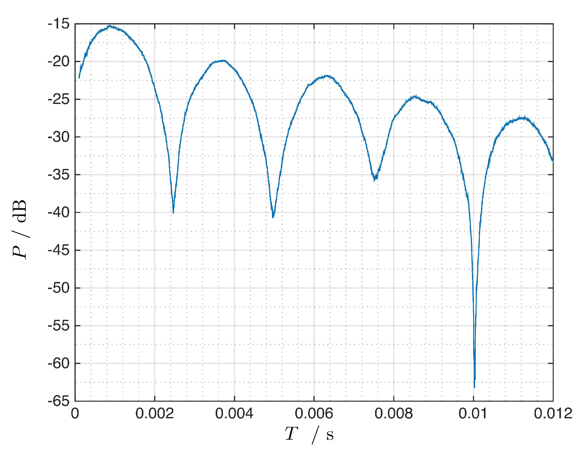
Figure 4 illustrates the Doppler extraction algorithm at which a section of duration T m a x of the continuous noise signals is extracted to a buffer and evaluated by a series of K matched filters of different durations T ( k ) . It is assumed that the maximum available matched filter durations is limited to
0 < T ( k ) T m a x ,
with T m a x representing the maximum available segment duration of the signals. The rate of the parameter T and the power of the echo signal mainly influence the depth of the zero positions in the function R s g ( τ D ) ( T ) from which, as a last step in the schematic, the Doppler frequency of the target at a given distance D is extracted. In practical applications, the zero-points are indicated by local minima of (22) instead of exact zero values.
The method only requires that the target needs to be the sole Doppler-shifted echo in its range cell. Static echoes like stationary clutter are expected to limit the depth of the local minima of (22) which is less damaging to the evaluation method as would be two significantly different Doppler modulations in the same range-cell, a situation being quite unlikely to endure for a longer period.
Section 4 presents an experiment creating suitable data to test the described signal processing method. The scheme is particularly suitable for (pseudo-)random signals where the signal bandwidth is not affected by the choice of the segment duration. It is important to emphasize again that the different matched filters, applied in this method, use the same set of data.

4. Experiment

The experimental data were obtained by a noise radar demonstrator initially designed to investigate the influence of the proper motion of a moving radar platform on noise radar signals. This experimental set-up and the feasibility of the usage of noise radar on moving platforms was first presented in [36].
The experiment uses a radar demonstrator that operates in the X-band with a very low transmitter power of about 25 mW. The waveform used during the experiment was a band-limited Gaussian noise signal with a bandwidth of B = 50 MHz and a duration of 400 ms. This duration, interpreted as a pulse repetition interval, corresponds to an unambiguous range of 60 million meters and, thus, can be considered as non-repetitive from the radar point of view. Two standard horn antennas are mounted to the moving platform using a modified bicycle carrier and a large absorbent block as shown in Figure 5. The main unit of the radar demonstrator was located inside the trunk of the car and was controlled by a radar operator. A different person is required to drive this set-up. For safety reasons, the experiments took place on a temporarily closed runway.
The used moving radar platform produced particularly suitable data to illustrate the new signal processing method of Doppler extraction, because these data contain a minimum amount of static echoes. The scene of the experiment is illustrated in Figure 6: the radar platform overtakes a cooperatively driven truck that moved with a constant speed, 25 km/h less than the velocity of the radar platform. In this set-up, the directions of motion of both vehicles were identical and, thus, the measured relative radial velocity equals the difference in true speeds.
The measurement results, presented in Section 5, refer to the non-standard unit of km/h which allows for a direct mapping of the radar measurement and the tachometer values of the two vehicles.

5. Results

Two different recordings of the scene were evaluated at different ranges between the radar platform and the moving target. For both sets of data, a maximum duration of T m a x = 12 ms of recorded data was deliberately chosen in agreement with the considerations made in Section 1.2.
Figure 7 presents the evaluation of R s g ( τ D ) ( T ) , as defined in (22), for a target distance of D = 51 m. The zero points of the curve are reasonably deep and their mutual distance corresponds to a mean Doppler shift of f D = 441 Hz, resulting in a relative velocity of
v r , 1 = 7.056 m / s ,
that, being equivalent to 25.4 km/h, matches the value of the speed difference of both vehicles. Table 2 presents the four Doppler frequencies obtained by pairwise computing the distances of subsequent zero positions. The standard deviation of the measured data is equal to 10 Hz resulting in an accuracy of Δ v r = 0.16 m/s (0.58 km/h).
The second recording was made at a mutual distance of D = 141 m between the radar platform and the target vehicle. The analysis creates a function similar to that of Figure 8. This more distant measurement indicates that at increasing target distances, noise adds to the curve due to the decreasing signal power on receive but still the zero positions are very pronounced.
A comparison of both measurements leads to the observation of a marginal velocity change from v r , 1 = 25.4 km/h to v r , 2 = 22.84 km/h, reasoned by the fact that at D = 141 m the radar platform gradually approached the end of the track and initiated a braking process. This marginal change in velocity creates a significant shift of the zero points in Figure 8 compared to those of Figure 7, which is easily noticeable by eye.
Thus, the experimental data show the high sensitivity of (22) even on marginal velocity changes underlining the precision of the velocity measurement achievable by the method of this paper.

6. Discussion

This work has presented a signal processing method which allows for a precise Doppler measurement by multiple matched filters applied to the same set of data. The computational effort required by the many matched filters pays off by a significantly reduced illumination time of the target as compared to conventional Doppler determination by Fourier analyses. The requirements for the presented Doppler processing approach are three-fold:
1.
The waveform needs to have a (pseudo-)random modulation that covers the full signal bandwidth at all times.
2.
The waveform has to be free of range-Doppler coupling, usually indicated by a thumbtack-like shape of the ambiguity function.
3.
The target of interest has to be the sole target in the corresponding range cell.
The first two requirements are inherently met by noise radar signals. The third requirement strongly depends on the radar application and is expected to be the decision-maker if the proposed processing scheme is useful in a particular application or not.
The experiment shows an example in which the presented Doppler procedure applies well to real-world data. In the following, the experimental results are discussed with a Doppler measurement based on a conventional Fourier analysis. Section 5 stated that the duration of the data recording was deliberately limited to 12 ms. This maximum available coherent processing interval, according to (2), would limit the Doppler resolution to
Δ f D = 83 Hz ,
using a Doppler filter bank (implemented by an FFT) to extract the Doppler information. This value is equivalent to velocity increments of
Δ v r = 4.8 km / h
for the X-band radar used during the experiments. In noise radar technology, the cross-ambiguity function CAF [3] is a suitable signal processing approach for which the PRI can be set to the sampling rate of the signal and a Doppler analysis of a single range cell may be performed without Doppler-ambiguities by
F { m D ( t ) } = T / 2 T / 2 m D ( t ) e 2 π f t d t ,
where
m D ( t ) = s ( t ) g * ( t τ D )
is computed for a single target distance D, respectively for the corresponding delay value τ D . Figure 9 shows the results of a Doppler analysis performed by the cross-ambiguity function and a coherent processing interval of 12 ms. The FFT, in the current example, has a corresponding length of 600,000 samples and shows a resolution of Δ v r = 4.8 km/h as expected for this particular CPI.

7. Outlook

The following paragraphs briefly introduce potential future applications of the findings of this work and sketch planned future investigations in the context of the presented signal processing algorithm.

7.1. Marine Navigation Radars

The results indicate that the presented Doppler analysis method might enable precise velocity measurements even in radar sets operating at lower frequency bands. Thus, the proposed processing scheme might result in an increased performance, for instance in the case of marine navigation radars. Today, modern long-range S-band marine radars have advanced from magnetrons towards solid-state technology like the FAR-3000 NXT of the company Furuno [37] and, thus, already provide the basic technology for a potential update towards continuous radar emissions in the future.

7.2. Radar Ressource Management

Modern radar systems and multi-function RF sensors (MFRFS) complete several different, concurrent tasks performed in an interlocked (preferably even simultaneous) manner and, thus, demand for an efficient use of the sensor’s resources. A conventional Doppler analysis, performed at high precision, would consume important RF resources for a long period. The presented signal processing approach, instead, requires only a single and comparably short recording of the target of interest. These data are analyzed offline by, unquestionably, a computationally intense method. But during the analysis, the sensor is free to perform other tasks.

7.3. Design of Doppler-Tolerant Noise Radars

Focusing on continuous emission noise radar, theoretical considerations on the Doppler tolerance were made in this work and a method for its quantification was formulated. Generally, a proper segmentation of the continuous noise radar data is identified being the key method to control the Doppler tolerance. For a given application with given expectations on the target velocities, the presented achievements on the Doppler tolerance may be used to design a particular matched filter implementation in order to reduce the damaging effects of the low Doppler tolerance of noise radars by respecting the Doppler-tolerant duration of the matched filter. Additionally, this work provides a measure to identify radar scenarios in which Doppler computations are important not only if the velocity of moving targets shall be extracted but also for the compensation of the proper motion of a significantly moving radar platform.

7.4. Conclusions and Future Work

A deep investigation on the Doppler tolerance of CE noise radar has led to a series of interesting conclusions which have the potential to accelerate the productionization of noise radars. Futhermore, by enabling precise velocity measurement with limited RF resources, this work has introduced a new advantage of noise radar against conventional deterministic radar waveforms.
Further investigations will be made to increase the performance of the presented processing scheme. One aim is to reduce the number of required matched filters. For this task, state-of-the-art signal processing approaches like genetic algorithms will be taken into consideration. A second aim is to enhance the precision of the determination of the zero points and, thus, to further increase the Doppler precision. The presented experiment was tailored to the needs of demonstrating the general principle of the Doppler extraction method under good conditions, that is, the RCS of the target was immense and the distance was quite short. For smaller targets and for larger distances an accurate determination of the position of the zero points is an ongoing work that will be accompanied with a new experiment when it is ready to be published.

Funding

This research was funded by the WTD-81 of the German Bundeswehr.

Acknowledgments

The author would like to thank Gaspare Galati, Tor Vergata University of Rome, for his guidance during the PhD work that has laid the basis of the presented research. Furthermore, the experiments would not have been possible without the gratefully acknowledged help of the German Bundeswehr, WTD-81 and WTD-41. A special thank goes to the drivers of the experimental platform, David Wegner and Marco Dresen, both working at Fraunhofer FHR.

Conflicts of Interest

The author declares no conflict of interest.

References

  1. Horton, B.M. Noise-Modulated Distance Measuring Systems. Proc. IRE 1959, 47, 821–828. [Google Scholar] [CrossRef]
  2. Kulpa, K.; Lukin, K.; Miceli, W.; Thayaparan, T. Signal Processing in Noise Radar Technology. IET Radar Sonar Navig. 2008, 2, 229–232. [Google Scholar] [CrossRef]
  3. Kulpa, K. Signal Processing in Noise Waveform Radar; Artech House: Boston, MA, USA, 2013. [Google Scholar]
  4. Pace, P. Detecting and Classifying Low Probability of Intercept Radar; Artech House: Boston, MA, USA, 2009. [Google Scholar]
  5. Galati, G.; Pavan, G.; De Palo, F. Compatibility Problems Related with Pulse-Compression, Solid-State Marine Radars. IET Radar Sonar Navig. 2016, 10, 791–797. [Google Scholar] [CrossRef]
  6. Xu, Z.; Shi, Q. Interference Mitigation for Automotive Radar Using Orthogonal Noise Waveforms. IEEE Geosci. Remote. Sens. Lett. 2018, 15, 137–141. [Google Scholar] [CrossRef]
  7. Malanowski, M. Signal Processing for Passive Bistatic Radar; Artech House: Norwood, MA, USA, 2019. [Google Scholar]
  8. Wasserzier, C. Noise Radar on Moving Platforms. Ph.D. Thesis, Tor Vergata University of Rome, Rome, Italy, 2020. [Google Scholar]
  9. Lerner, R. A Matched Filter Detection System for Complicated Doppler Shifted Signals. IRE Trans. Inf. Theory 1960, 6, 373–385. [Google Scholar] [CrossRef]
  10. Aubry, A.; De Maio, A.; Naghsh, M.M. Optimizing radar waveform and Doppler filter bank via generalized fractional programming. IEEE J. Sel. Top. Signal Process. 2015, 9, 1387–1399. [Google Scholar] [CrossRef]
  11. Richards, M.A.; Scheer, J.; Holm, W.A.; Melvin, W.L. Principles of Modern Radar; Scitech Publishing: Edison, NJ, USA, 2010. [Google Scholar]
  12. Cheney, M.; Borden, B. Fundamentals of Radar Imaging; SIAM: Philadelphia, PA, USA, 2009. [Google Scholar]
  13. Stimson, G.W. Introduction to Airborne Radar, 2nd ed.; SciTech Publishing Inc.: Raleigh, NC, USA, 1998. [Google Scholar]
  14. Levanon, N.; Mozeson, E. Radar Signals; John Wiley & Sons: Hoboken, NJ, USA, 2004. [Google Scholar]
  15. Blighter Surveillance Systems. B400 Series Radars—Datasheet; BSS-0814; Blighter Surveillance Systems: Great Chesterford, UK, 2020. [Google Scholar]
  16. JRC Japan Radio Co., Ltd. Marine Radar JMR-5400 Series—Datasheet; JRC Japan Radio Co., Ltd.: Nakano, Japan, 2017. [Google Scholar]
  17. van Keuk, G.; Blackman, S.S. On phased-array radar tracking and parameter control. IEEE Trans. Aerosp. Electron. Syst. 1993, 29, 186–194. [Google Scholar] [CrossRef]
  18. Brandfass, M.; Boeck, M.; Bil, R. Multifunctional AESA Technology Trends–A Radar System Aspects View. In Proceedings of the 2019 IEEE International Symposium on Phased Array System Technology (PAST), Waltham, MA, USA, 15–18 October 2019; pp. 8138–8143. [Google Scholar]
  19. Wasserzier, C.; Worms, J.G.; O’Hagan, D.W. How Noise Radar Technology Brings Together Active Sensing and Modern Electronic Warfare Techniques in a Combined Sensor Concept. In Proceedings of the IEEE Sensor Signal Processing for Defence Conference (SSPD), Brighton, UK, 9–10 May 2019; pp. 1–5. [Google Scholar] [CrossRef]
  20. Rihaczek, A.W. Doppler-tolerant Signal Waveforms. Proc. IEEE 1966, 54, 849–857. [Google Scholar] [CrossRef] [Green Version]
  21. Yan, X.; Hao, X.; Xu, F.; Geng, X. Ranging Accuracy and Doppler Tolerance of CW Signal Based on Pseudo-Random Code Bi-Phase Modulation. In Proceedings of the 4th International Conference on Wireless Communications, Networking and Mobile Computing, Dalian, China, 12–14 October 2008; pp. 1–4. [Google Scholar] [CrossRef]
  22. Wang, L.; Fu, X.; Shi, L.; Li, T.; Gao, M. Radar Waveform Design under the Constraint of Auto-Correlation, Orthogonality and Doppler Tolerance. In Proceedings of the IET International Radar Conference 2013, Xi’an, China, 14–16 April 2013; pp. 1–4. [Google Scholar] [CrossRef]
  23. Qazi, F.A.; Fam, A.T. Doppler Tolerant and Detection Capable Polyphase Code Sets. IEEE Trans. Aerosp. Electron. Syst. 2015, 51, 1123–1135. [Google Scholar] [CrossRef]
  24. Chen, R.C.; Higgins, T. Doppler Tolerant Time Separated Golay Waveforms. In Proceedings of the International Waveform Diversity Design Conference (WDD), Kauai, HI, USA, 22–27 January 2012; pp. 166–171. [Google Scholar] [CrossRef]
  25. Nguyen, H.D.; Coxson, G.E. Doppler Tolerance, Complementary Code Sets, and Generalised Thue-Morse Sequences. IET Radar Sonar Navig. 2016, 10, 1603–1610. [Google Scholar] [CrossRef]
  26. Yang, J.; Sarkar, T.K. A New Doppler-Tolerant Polyphase Pulse Compression Codes Based on Hyperbolic Frequency Modulation. In Proceedings of the IEEE Radar Conference, Boston, MA, USA, 17–20 April 2007; pp. 265–270. [Google Scholar] [CrossRef]
  27. Setlur, P.; Hollon, J.; Arasu, K.T.; Rangaswamy, M. On a Formal Measure of Doppler Tolerance. In Proceedings of the IEEE Radar Conference, Seattle, WA, USA, 8–12 May 2017; pp. 1751–1756. [Google Scholar] [CrossRef]
  28. Franken, G.E.A.; Nikookar, H.; Genderen, P.V. Doppler Tolerance of OFDM-Coded Radar Signals; European Radar Conference (EuRad): Manchester, UK, 2006; pp. 108–111. [Google Scholar] [CrossRef]
  29. Woodward, P.M. Probability and Information Theory with Applications to Radar; Pergamon Press Ltd.: London, UK, 1953. [Google Scholar]
  30. De Palo, F.; Galati, G.; Pavan, G.; Wasserzier, C.; Savci, K. Introduction to Noise Radar and its Waveforms. Sensors 2020, 20, 5187. [Google Scholar] [CrossRef] [PubMed]
  31. Galati, G. (Ed.) Advanced Radar Techniques and Systems; Institution of Electrical Engineers (IEE): London, UK, 1993. [Google Scholar]
  32. Skolnik, M. Radar Handbook, 3rd ed.; McGraw-Hill: New York, NY, USA, 2008. [Google Scholar]
  33. Brandwood, D. Fourier Transforms in Radar and Signal Processing; Artech House: Norwood, MA, USA, 2012. [Google Scholar]
  34. Galati, G.; Pavan, G.; Wasserzier, C. Optimal Processing in Noise Radar: Implementation Problems. In Proceedings of the Signal Processing Symposium, Krakow, Poland, 17–19 September 2019. [Google Scholar]
  35. Navico America and Simrad Yachting. Broadband 4G Radar—Datasheet; Navico America and Simrad Yachting: Tusla, OK, USA, 2011. [Google Scholar]
  36. Wasserzier, C.; Galati, G. First Experimental Results on the Feasibility of Noise Radar Systems on Fast Moving Platforms. Electron. Lett. 2019, 55, 344–345. [Google Scholar] [CrossRef]
  37. Furuno. Chart Radar—FAR-3000 Series. CA000001414. 2004. Available online: https://www.furuno.com/files/Brochure/105/upload/FAR-3000%20series%20Brochure.pdf (accessed on 1 September 2020).
Figure 1. Illustration of the thumbtack-like ambiguity function of a close-to-ideal noise waveform with wide bandwidth and long duration. Neither range nor Doppler ambiguities exist and range-Doppler coupling does not occur.
Signals 02 00003 g001
Figure 2. The signal u r ( t ) is modeled by limiting the duration, that is, by segmenting, a signal n ( t ) that itself represents a band-limited signal extracted from an (idealized) Gaussian noise source N 0 .
Signals 02 00003 g002
Figure 3. The matched filter of duration T 0 applied to noise radar signals creates a sinc-shaped Doppler characteristic in the zero-delay cut of the ambiguity function χ ( τ = 0 , f D ) 2 . The Doppler loss L r ( f D ) is higher than 3 dB for f D > 0.443 T 0 as indicated by the dashed line.
Signals 02 00003 g003
Figure 4. The Doppler extraction algorithm utilizes a set of matched filters (each having a different duration 0 < T ( k ) T m a x ) to the same set of noise radar data in order to extract the Doppler frequency f D of a target in a given distance D.
Signals 02 00003 g004
Figure 5. The radar was mounted to the rear of a standard car for moving-platform experiments on a temporarily closed runway.
Signals 02 00003 g005
Figure 6. The radar platform (white) overtakes a truck (red). The velocities differ by 25 km/h, according to the tachometer values.
Signals 02 00003 g006
Figure 7. The Doppler extraction method applied to radar data obtained for a target in a distance of D = 51 m.
Signals 02 00003 g007
Figure 8. A second measurement recorded a few moments later with a target distance of D = 141 m shows that a marginal variation of the velocity results in significantly different positions of the zero points relative to the previous measurement.
Signals 02 00003 g008
Figure 9. Result of an Fast Fourier Transform (FFT)-based Doppler analysis using a digital Fourier transform of 6 × 10 5 points length.
Signals 02 00003 g009
Table 1. Common radar targets to be detected by an example X-Band noise radar having a Doppler tolerance of f 3 d B = 443 Hz defined by a required coherent processing interval of T r = 1 ms. The Doppler-tolerant segment duration states the interval the matched filter of the radar must not exceed in order to instead assure a Doppler tolerance with respect to the particular targets.
TargetVelocityDoppler Frequency f D < f 3 dB Doppler-Tolerant
f D Segment Duration
sailing boat7 knots (3.6 m/s)240 Hzyes (×)1.8 ms
slow car30 km/h (8.3 m/s)553 Hzno (  )800 μ s
fast car130 km/h (36 m/s)2.4 kHzno (  )184 μ s
aircraftmach 1 (343 m/s)22.8 kHzno (  )19 μ s
Table 2. The mutual distances between the four zero points of Figure 7 allow for a determination of the echo’s Doppler frequency.
Zero PositionCorresponding Doppler Frequency
2454.75 Hz
3439.75 Hz
4440.33 Hz
5430.48 Hz
Publisher’s Note: MDPI stays neutral with regard to jurisdictional claims in published maps and institutional affiliations.

