Article

Investigating the Benefits of Vector-Based GNSS Receivers for Autonomous Vehicles under Challenging Navigation Environments

by
Haidy Y. F. Elghamrawy
1,2,*,
Mohamed Tamazin
3 and
Aboelmagd Noureldin
2,4
1
Department of Electrical and Computer Engineering, Royal Military College of Canada, Kingston, ON K7K 7B4, Canada
2
Department of Engineering Mathematics and Physics, Cairo University, Cairo 12613, Egypt
3
Department of Electronics and Communications, Arab Academy for Science, Technology and Maritime Transport, P.O. Box 1029, Alexandria, Egypt
4
School of Computing, Queen’s University, Kingston, ON K7L 2N8, Canada
*
Author to whom correspondence should be addressed.
Signals 2020, 1(2), 121-137; https://doi.org/10.3390/signals1020007
Submission received: 15 September 2020 / Revised: 24 September 2020 / Accepted: 28 September 2020 / Published: 1 October 2020

Abstract

:
There is a growing demand for robust and accurate positioning information for various applications, including the self-driving car industry. Such applications rely mainly on the Global Navigation Satellite System (GNSS), including the Global Positioning System (GPS). However, GPS positioning accuracy relies on several factors, such as satellite geometry, receiver architecture, and navigation environment, to name a few. In urban canyons in which there is a significant probability of signal blockage of one or more satellites and/or interference, the positioning accuracy of scalar-based GPS receivers drastically deteriorates. On the other hand, vector-based GPS receivers exhibit some immunity to momentary outages and interference. Therefore, it is becoming necessary to consider vector-based GPS receivers for several applications, especially safety-critical applications, including next-generation navigation technologies for autonomous vehicles. This paper investigates a vector-based receiver’s performance and compares it to its scalar counterpart in signal degraded conditions. The realistic simulation experiments in this paper are conducted on GPS L1 C/A signals generated using the SpirentTM simulation system to create a fully controlled environment to examine and validate the performance. The results show that the vector tracking system outperforms the scalar tracking in terms of position and velocity estimation accuracy in signal-degraded environments.

1. Introduction

Satellite-based positioning has gained a lot of attention due to its integration into many aspects of our daily activities. The Global Positioning System (GPS) has become a crucial part of numerous devices and applications, such as routing, vehicular Internet of Things (IoT), rescue and emergency services and future self-driving. One of the most well-known emerging applications nowadays that rely mainly on GPS is the autonomous vehicles in which there is a pivotal need for accurate and undisturbed navigation solutions. In such applications, a failure of the positioning service will potentially result in serious safety issues. Furthermore, countless current applications rely mainly on GPS such as intelligent transportation, tracking people, devices, pets and nearby area searching such as museums, oil stations, hospitals and restaurants. The widespread use and popularity of applications that demand GPS have led to the need for reliable, uninterrupted and accurate positioning and navigation services, which was the primary motivation for this research. Additionally, the flexibility associated with software receivers’ use compared to hardware receivers was another stimulus for the research in this paper.
GPS signals are received by receiver antennae below the noise floor, which makes them highly susceptible to in-band intentional, unintentional and malicious interference, even with the fact that GPS signals employ the direct sequence spread spectrum (DSSS) modulation technique, which gives them inherent robustness to interference signals. Jamming is considered one of the significant threats to users of GPS services [1,2] because it can severely affect the GPS receiver, causing unreliable and erroneous navigation solutions, and a loss of integrity and availability of satellite signals. In some cases, jammers could cause the receiver to undergo a complete outage. Moreover, high-power jammers can hinder the usage of GPS over a large area in the vicinity of the jammer [3,4].
This paper investigates the performance of a scalar- and vector-based software-defined receiver (SDR) in harsh navigation environments to provide a robust, continuous and reliable performance that can be further integrated with other navigation sensors to improve the overall system performance. The performance is assessed in highly degraded signal environments in which the signal power is highly attenuated and in the presence of interference signals.
In this paper, several quasi-real static and dynamic simulated scenarios are collected and processed by the SDR in both scalar and vector modes for performance comparison purposes. In these scenarios, the signal strength of one or more satellites is attenuated by 10–20 dB to assess the performance of the receiver in degraded conditions. The results show the superiority of vector tracking (VT) loops compared to scalar tracking (ST) loops in terms of bridging momentary outages in one or more satellites and re-locking to satellites’ signals in the presence of jamming.

2. Literature Review

The author in [5] introduced a novel integration scheme for the discriminator-based multipath mitigation technique and the VT loop. The proposed method was evaluated using real intermediate frequency (IF) signals collected in dynamic and static scenarios. The augmented receiver outperformed standalone VT and standalone ST concerning position estimation accuracy. Compared to the integration of ST with the multipath discriminator correlator, the minimum and maximum enhancements of the introduced integration scheme are 1.13 dB and 2.26 dB in terms of the tracking threshold, as noted in four-satellite and seven-satellite scenarios, respectively. The vector delay lock loop (VDLL) performance in multipath mitigation in an urban environment was assessed in [6]. Based on the findings of the paper, the VT loop identified the presence of a multipath based on the value of the variance of the measurement noise.
Moreover, VDLL exhibited an enhanced performance with respect to position accuracy compared to ST loops, even in the presence of severe multipath conditions. Kim et al., in [7], introduced an adaptive VT loop to minimize the effect of poor quality channels on the performance of VT. They proposed a rescaling method that rescales the measurement covariance matrix of the navigation filter. This adaptive implementation of VT has shown better positioning accuracy without any additional computational complexity. The VT loops in [8] were able to track blocked satellites’ signals without the need for re-acquisition, which, in turn, resulted in a significant enhancement in the computational demands of the software receiver. A performance comparison between vector delay frequency lock loop (VDFLL), VDLL, and ST was carried out in [9]. Based on the results, VDFLL was more robust to transmission disturbances such as multipath and high dynamics.
Furthermore, it outperformed other architectures in both tracking and navigation domains. The authors in [10] introduced two multi-pole complex adaptive infinite impulse response (IIR) and finite impulse response (FIR) notch filtering techniques in a vector-based global navigation satellite system (GNSS) receiver to suppress a continuous wave (CW) jamming signal. The proposed method was able to suppress the jamming signal based on the carrier phase measurements. In [11], a performance assessment of VT loops in the presence of radiofrequency (RF) interference was carried out. Their interference signals were examined in terms of additive white Gaussian noise (AWGN), CW, and ultra-wideband (UWB). VT loops outperformed ST in terms of position accuracy and tracking performance and position accuracy. Moreover, VT loops provided a gain of 5 dB in the carrier-to-noise ratio (C/N0) compared to ST loops. In [12], VDFLL showed an outstanding performance in terms of carrier tracking, C/N0 and position accuracy in dense foliage and extreme urban canyon environments.

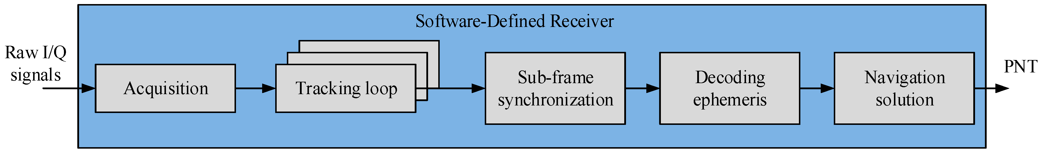
3. GPS Software-Defined Receiver

Figure 1 shows an overview of an SDR architecture. The first aim of an SDR is to detect the visible satellites and roughly estimate the received signal’s code phase and carrier frequency. Later, each satellite parameter will be tracked to refine these estimates and keep a lock on them. Then, the tracking loops’ output is utilized to calculate the GPS measurements, which are pseudo-ranges and pseudo-range rates. In addition, the navigation data are decoded to extract the ephemeris information and, consequently, compute the position of all available satellites. Eventually, the SDR will calculate the Position, Navigation and Timing (PNT) solutions based on the GPS measurements along with the satellite position information. Software processing offers some level of customization and flexibility when compared to hardware implementation using an application-specific integrated circuit (ASIC) that has traditionally been used to realize the signal processor part of the receiver [13]. Moreover, software processing lessens the cost and time consumption accompanying hardware prototyping.

4. Receiver Implementation Approaches

There are two implementation approaches for a GPS receiver that are explained in the following sections.

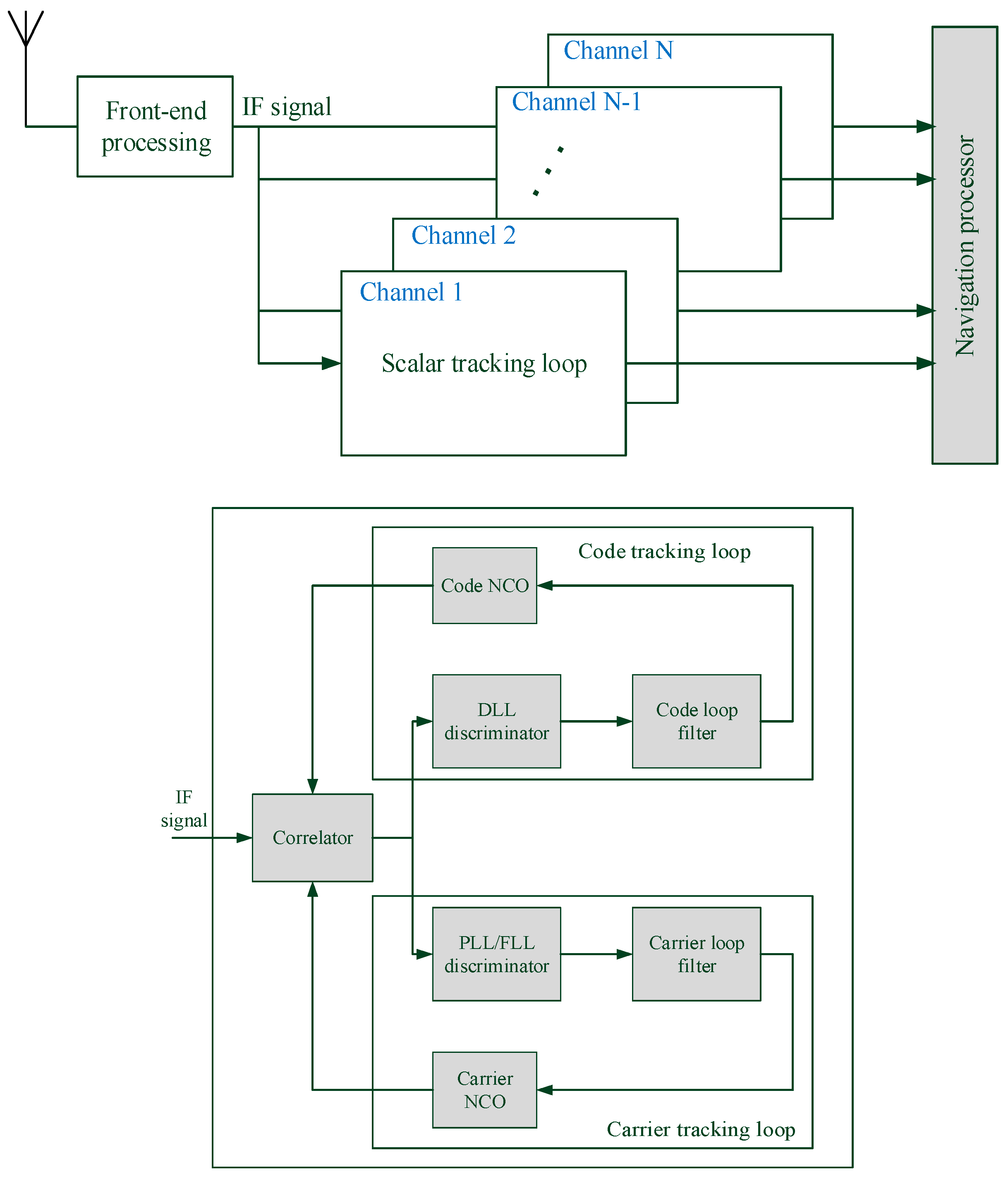
4.1. Scalar Tracking Receiver

Scalar tracking is based on a decentralized technique in signal tracking and navigation solution computation [14]. In this approach, each satellite is separately tracked in an independent channel, as shown in Figure 2. Therefore, there is no exchange information between the tracking loops or between the navigation and tracking modules. The tracking parameters of each channel are used to estimate the measurements of the tracked satellite. These measurements are then fed to the navigation processor; in turn, the navigation processor calculates the positioning information. This approach has some robustness as a faulty channel will not affect another channel. Moreover, it is simple and efficiently implemented [15]. However, it does not exploit the inherent coupling between the dynamics in each channel and the dynamics of the receiver [14].

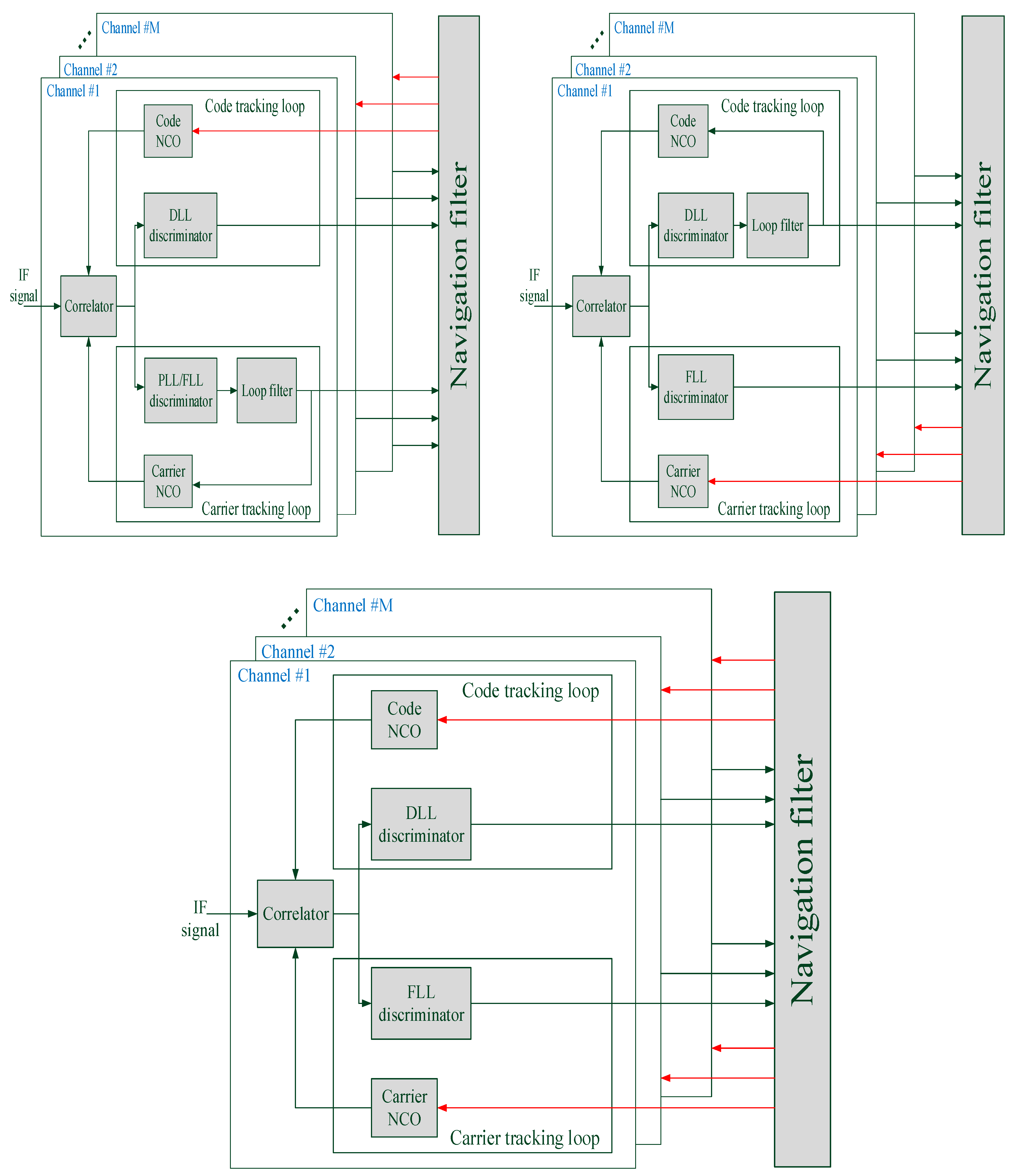
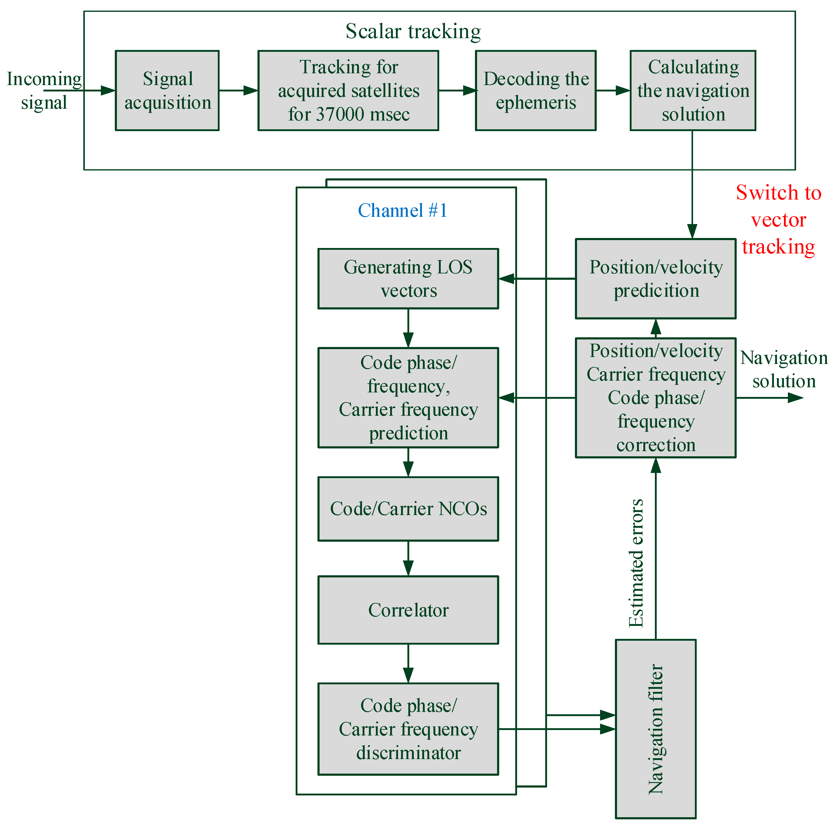
4.2. Vector Tracking Receiver

Unlike a scalar-based receiver, a vector-based receiver exploits a centralized approach as it combines both tracking and navigation into a single estimation problem. This tracking technique is based on the idea that each channel’s parameters, including code phase and carrier frequency/phase, are linked to the dynamics of the receiver by the line-of-sight (LOS) vectors [16]. The navigation solution is fed back to the tracking loops to drive the code and carrier numerically controlled oscillator (NCO) to exploit the coupling between the tracking and receiver’s position and velocity [17]. This VT architecture has some advantages over its scalar counterpart, including [17,18,19]:
  • Improved tracking performance, as the positioning solution is assisting the tracking,
  • Robustness to disturbances such as multipath, high dynamics and degradation in signal strength,
  • Some immunity to jamming,
  • Bridging momentary outages of one or more satellites.
However, these advantages come at the penalty of more complexity in the implementation of a vector-based receiver. In addition, a faulty channel will potentially affect all other channels due to inter-channel aiding, which might result in an overall deterioration in the performance of the receiver [15].

5. Vector Tracking Loop Architectures

VT can be implemented in three different approaches, as shown in Figure 3. The first architecture is a vector delay lock loop (VDLL) in which code phases are tracked through a centralized approach, while carrier tracking loops work independently. The second architecture is the vector frequency lock loop (VFLL), which handles carrier tracking in a centralized approach, while ST loops handle code phases. Finally, the vector delay frequency lock loop (VDFLL) utilizes a central filter, usually a Kalman filter (KF), to track both the code phase and the carrier frequency of all channels. In this paper, VDFLL is adopted to assess its performance in degraded signal environments.

Vector Tracking Module

Figure 4 shows a flow chart of the steps carried out by a vector-based GPS SDR. VT requires the knowledge of the code phase φ ^ k m , code frequency f ^ c o d e ,   k m , carrier frequency f ^ c a r r , k + 1 m , clock bias b r , k , clock drift d r , k , user position x k , user velocity v k and transmit time t t r ,   k m at the beginning of its operation. The subscript k denotes the time epoch, and the superscript m represents the mth satellite. In the beginning, ST is activated for thirty-seven seconds to be able to acquire and decode the ephemeris data and consequently compute the navigation solution to initialize the VT module with all the required parameters. The position and velocity are predicted based on the models described by the following equations [20]:
x ^ k + 1 = x k + Δ T   v k ,
v ^ k + 1 = v k ,
where ^ represents predicted value, and Δ T denotes the time interval between kth and (k + 1)th. Next, the code phase, the carrier frequency is predicted based on the expected user position, velocity, and the satellites position, velocity calculated from extracting the ephemeris [16].
φ ^ k + 1 m = φ m , k + [ Δ x k k + 1 m Δ T   v k ] T .   1 m , k + 1 + Δ T c ,
f ^ c o d e , k + 1 m = ( 1 + t d , k + [ v k m v k ] T .   1 k + 1 m ) f c o d e / c ,
f ^ c a r r , k + 1 m = ( 1 + t d , k + [ v k m v k ] T .   1 k + 1 m ) f c a r r / c ,
where Δ x k k + 1 m is the displacement vector of the m th satellite from epoch k to k   + 1 , c is the speed of light, v k m is the mth satellite velocity, 1 m , k + 1 is the LOS vector between the receiver and the m th satellite, f c o d e is the nominal code frequency (1.023 MHz for the C/A code) and f c a r r is the nominal carrier frequency (1575.42 MHz for GPS L1 signal). Afterwards, the local replicas of the code and carrier are generated based on the predicted code phase, and carrier frequency and these replicas are correlated with the incoming signal. Next, the code and carrier discriminators output the code phase and carrier frequency errors that correspond to the LOS projections of the errors between the actual position and velocity and their predicted counterpart (i.e., ( x k + 1 x ^ k + 1 ) . 1 k m and ( v k + 1 v ^ k + 1 ) . 1 k m ). The code phase error is expressed as a function of the user position error as follows
E c o d e , k = φ k m φ ^ k m + η k m = b r , k + [ x k + 1 x ^ k + 1 ] . 1 k m + η k m ,
where E c o d e , k is the code phase error, and η k m is the noise term.
Likewise, the relationship between carrier frequency error and user velocity error can be represented as follows:
E c a r r , k = f c a r r , k m f ^ c a r r , k m + w k m = Δ d r , k + [ v k + 1 v ^ k + 1 ] .   1 k m + w k m ,
where E c a r r , k represents the carrier frequency error, Δ d r , k is the difference between the clock drift at epoch k ( d r , k ) and epoch k 1 ( d r , k ) and w k m is the noise term. The position and velocity errors ( ( x k + 1 x ^ k + 1 ) , ( v k + 1 v ^ k + 1 ) ) are then used to improve the estimated position x ^ k + 1 and velocity v ^ k + 1 to compute the real position and velocity solution. These errors are estimated using KF, with the states of the system being position error ( δ x ) , clock bias ( b r ) , velocity error ( δ v ) and change in clock drift Δ d r . The position at time epoch k is assumed to be known; thus, the position error at time epoch ( k   +   1 ) can be obtained by the integration of the velocity error during ( k th ( k + 1 ) th ) time epochs; this time duration is set to be too short and thus it can be assumed that the velocity error is constant over this short period. Consequently, the position error can be determined by [16]
δ x k + 1 = Δ T   δ v k + ψ k + 1 ,
where ψ k + 1 is white Gaussian noise (WGN).
In a similar fashion, the velocity at time epoch k is assumed to be known; thus, the velocity error can be modeled as WGN. The velocity error at time epoch ( k   +   1 )   can be expressed as:
δ v k + 1 = ϱ k + 1 ,
where ϱ k + 1 is WGN.
The receiver clock bias is caused by the clock drift in the interval between ( k th ( k + 1 ) th ) time epochs, and hence it is modeled as a function of the clock drift. The clock bias and drift are expressed as:
b r , k + 1 = b r , k + Δ T ( d r , k + 1 d r , k ) ,
d r , k + 1 = d r , k + Δ d r , k
The change in the clock drift Δ d r , k can be modeled as WGN because GPS oscillators are of a very high quality and usually have a stable clock drift over a short period. According to Equations (8)–(11), the state model of the system can be represented in the matrix form as [16]:
[ δ x k + 1 δ y k + 1 δ z k + 1 b r , k + 1 δ v x , k + 1 δ v y , k + 1 δ v z , k + 1 Δ d r , k + 1 ] = [ 0 0 0 0 Δ T 0 0 0 0 0 0 0 0 Δ T 0 0 0 0 0 0 0 0 Δ T 0 0 0 0 1 0 0 0 Δ T 0 0 0 0 0 0 0 0 0 0 0 0 0 0 0 0 0 0 0 0 0 0 0 0 0 0 0 0 0 0 0 0 ] [ δ x k δ y k δ z k b r , k δ v x , k δ v y , k δ v z , k Δ d r , k ] + W k ,
where W k is WGN.
The measurements of the system are the outputs of the code and carrier discriminators which are expressed by Equations (6) and (7). Thus, the measurement model is represented in the matrix form as [16]:
[ E c o d e , k 1 E c o d e , k 2 E c o d e , k M E c a r r , k 1 E c a r r , k 2 E c a r r , k M ] = [ 1 x , k 1 1 y , k 1 1 z , k 1 1 0 0 0 0 1 x , k 2 1 y , k 2 1 z , k 2 1 0 0 0 0 1 x , k M 1 y , k M 1 z , k M 1 0 0 0 0 0 0 0 0 1 x , k 1 1 y , k 1 1 z , k 1 1 0 0 0 0 1 x , k 2 1 y , k 2 1 z , k 2 1 0 0 0 0 1 x , k M 1 y , k M 1 z , k M 1 ] [ δ x k δ y k δ z k b r , k δ v x , k δ v y , k δ v z , k Δ d r , k ] + ε k ,

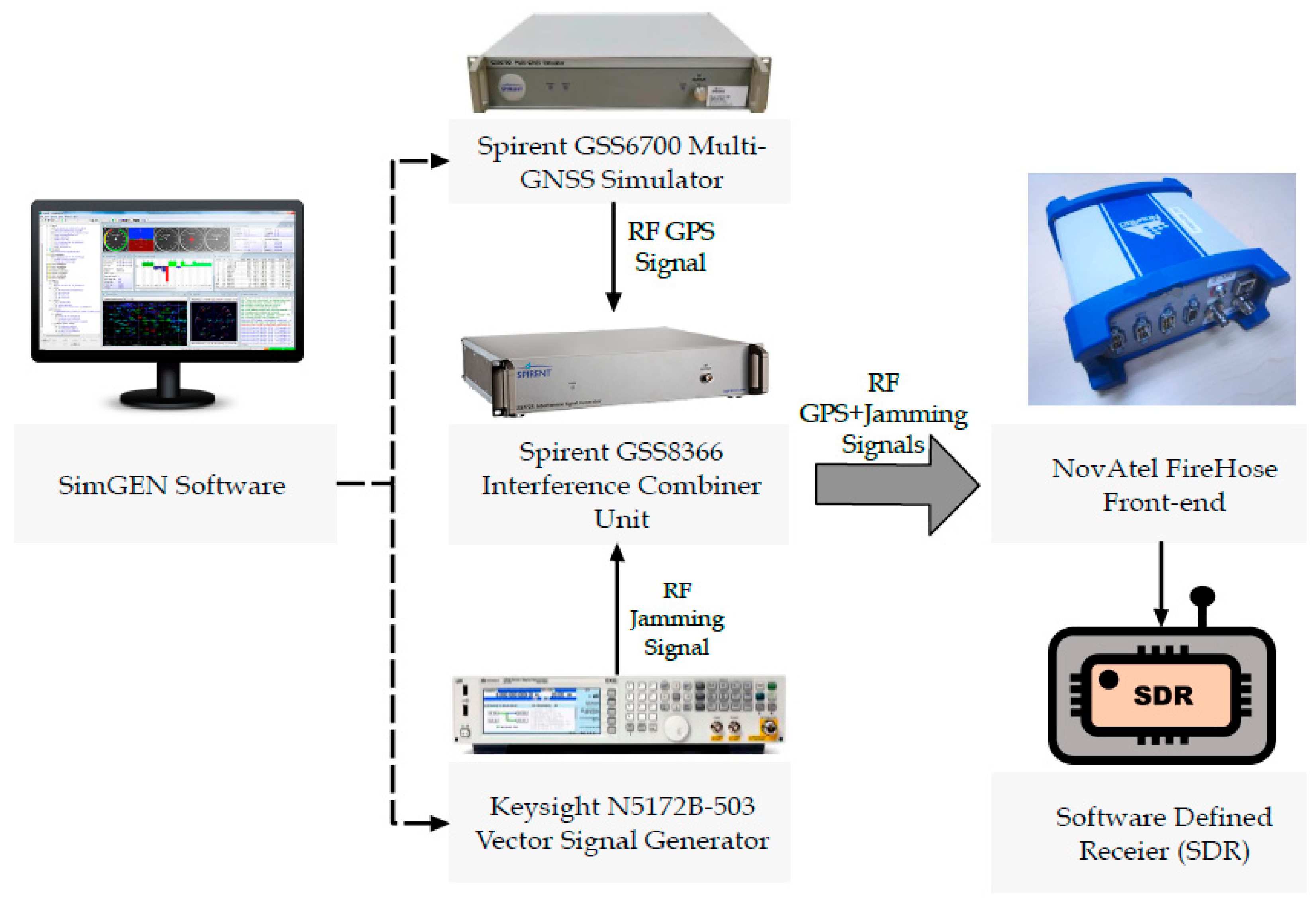
6. Hardware Experimental Setup

Figure 5 shows the experimental hardware setup. The SpirentTM GSS6700 GNSS simulation system [21] is utilized in this research to create a fully controlled environment to assess the performance of the vector-based GPS SDR in various signal degraded conditions using both static and dynamic scenarios. The SpirentTM simulation system is run by SimGENTM simulation software [22]. SimGENTM enables the simulation of terrain obscuration, several multipath scenarios, variable antenna reception parameters, the trajectory generation of air, sea, land and space vehicles, ionospheric and tropospheric degradation of GNSS signals, and several jamming signals, including continuous wave (CW), swept continuous wave (SCW), amplitude-modulated (AM) and frequency-modulated (FM) [23], to name a few. The output RF signal is equivalent to that from real satellites as if the antenna is mounted on a vehicle on an actual road trajectory at the location and time of the simulation. The jamming signal is generated using the Agilent interference signal generator (ISG) that is connected to SpirentTM GSS6700 via the SpirentTM GSS8366 interference combiner unit (ICU).
The output RF signal is then processed by FireHose D17088 front-end (FE) by NovAtel [24] to generate the raw in-phase (I) and quadrature-phase (Q) signals. Inside the FE, the received signal is downconverted from RF to baseband via several down-conversion stages. Next, the baseband signal is sampled and digitized using an analog-to-digital converter (ADC). The FireHose-FE can collect GPS L1/L2 signals at bandwidths of 2.5 MHz, 5.0 MHz, 10 MHz, and 20 MHz. Furthermore, the number of quantization bits can vary from 1-bit up to 8-bit. Eventually, the digital signal is sent to the computer using an ethernet connection. These data are stored for post-processing by the SDR.

7. Data Collection and Scenario Details

The data collection parameters of the SpirentTM simulator, FireHose FE and software receiver are outlined in Table 1, Table 2 and Table 3, respectively. The reference solution is obtained from the logs generated by the SpirentTM simulation system.

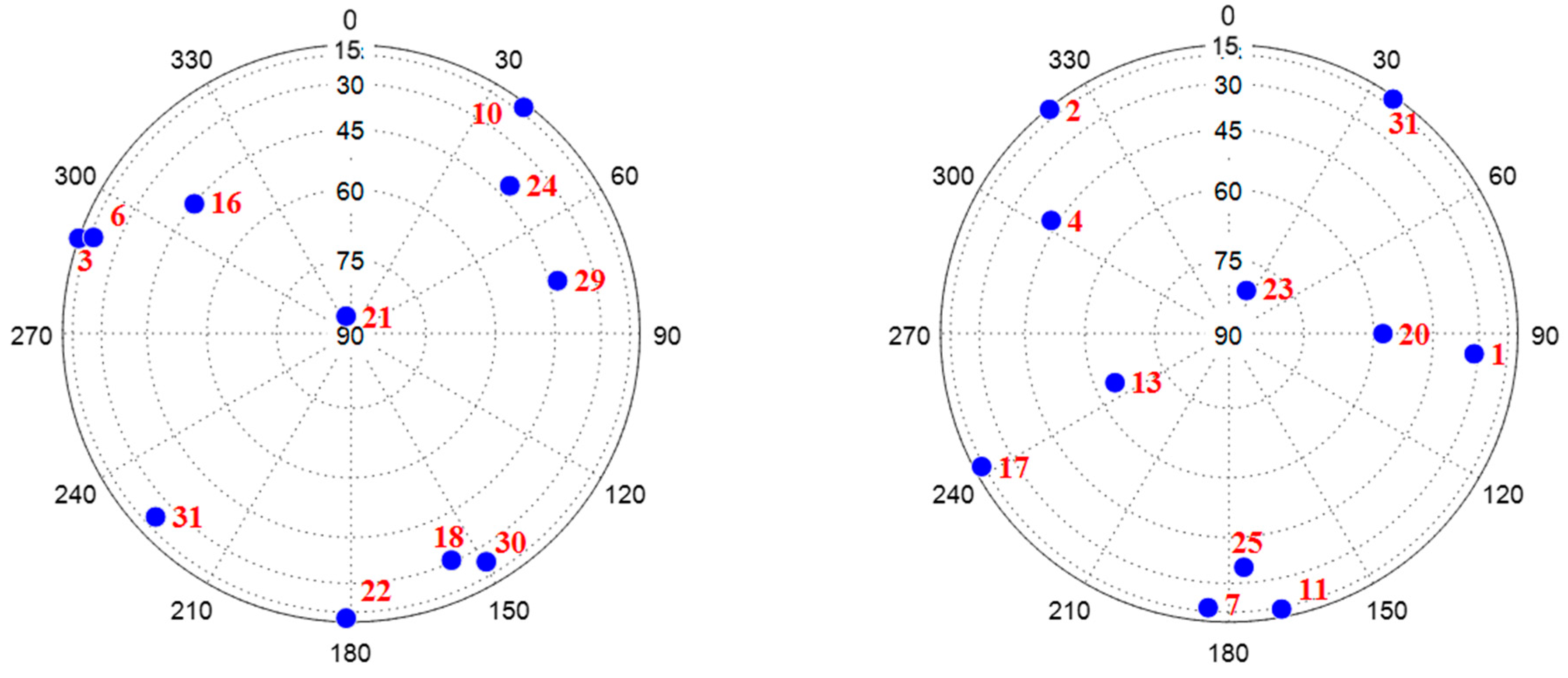
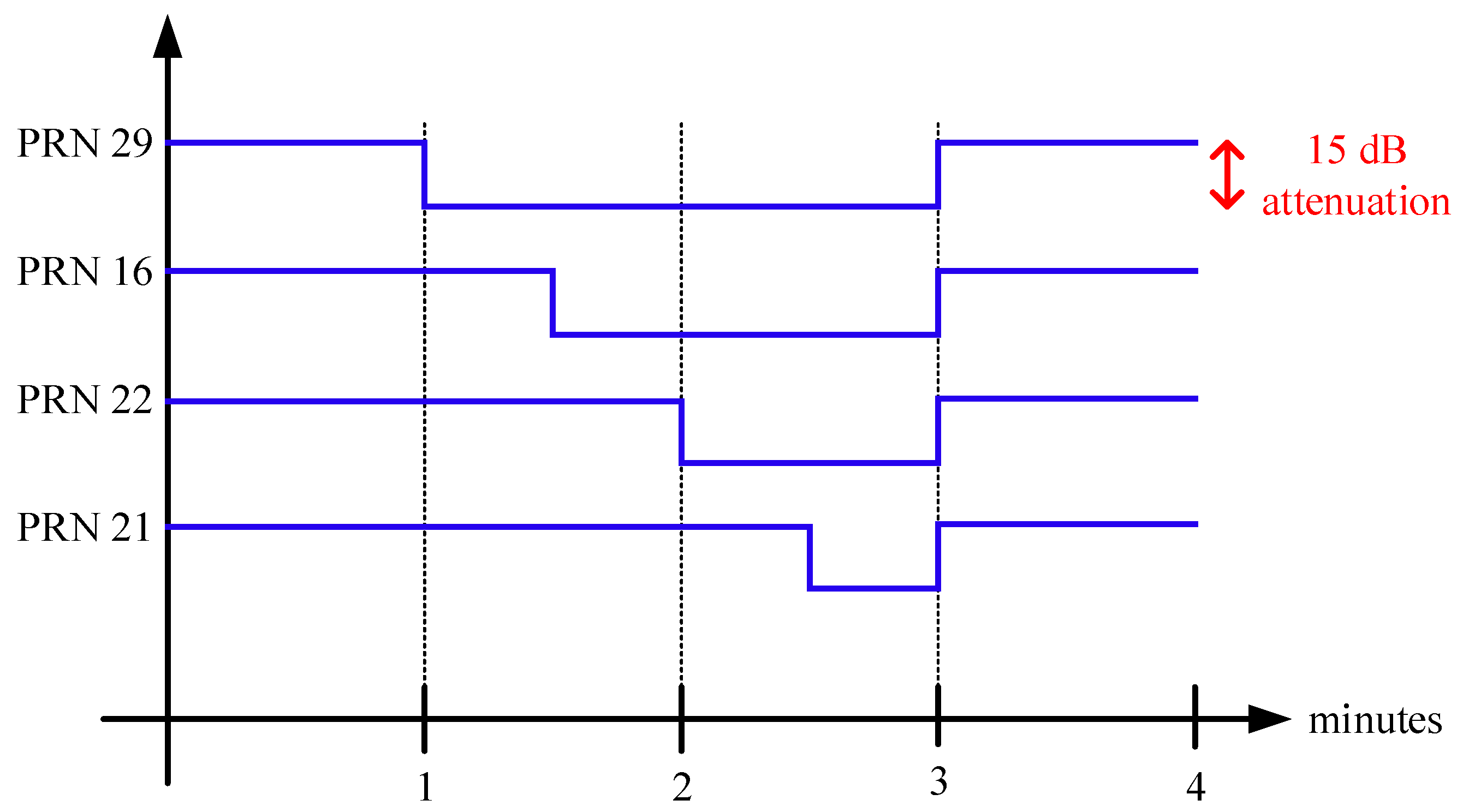
7.1. Static Scenario

The details of the static scenario are as follows:
  • Time of simulation: 2 September 2018 at 12:00:00 p.m.
  • Location: Washington Dullus Airport, VA, the United States at 38°57′11.6″ N latitude and 77°27′23.4″ W longitude.
  • The number of visible GPS satellites: 11, as shown in Figure 6.

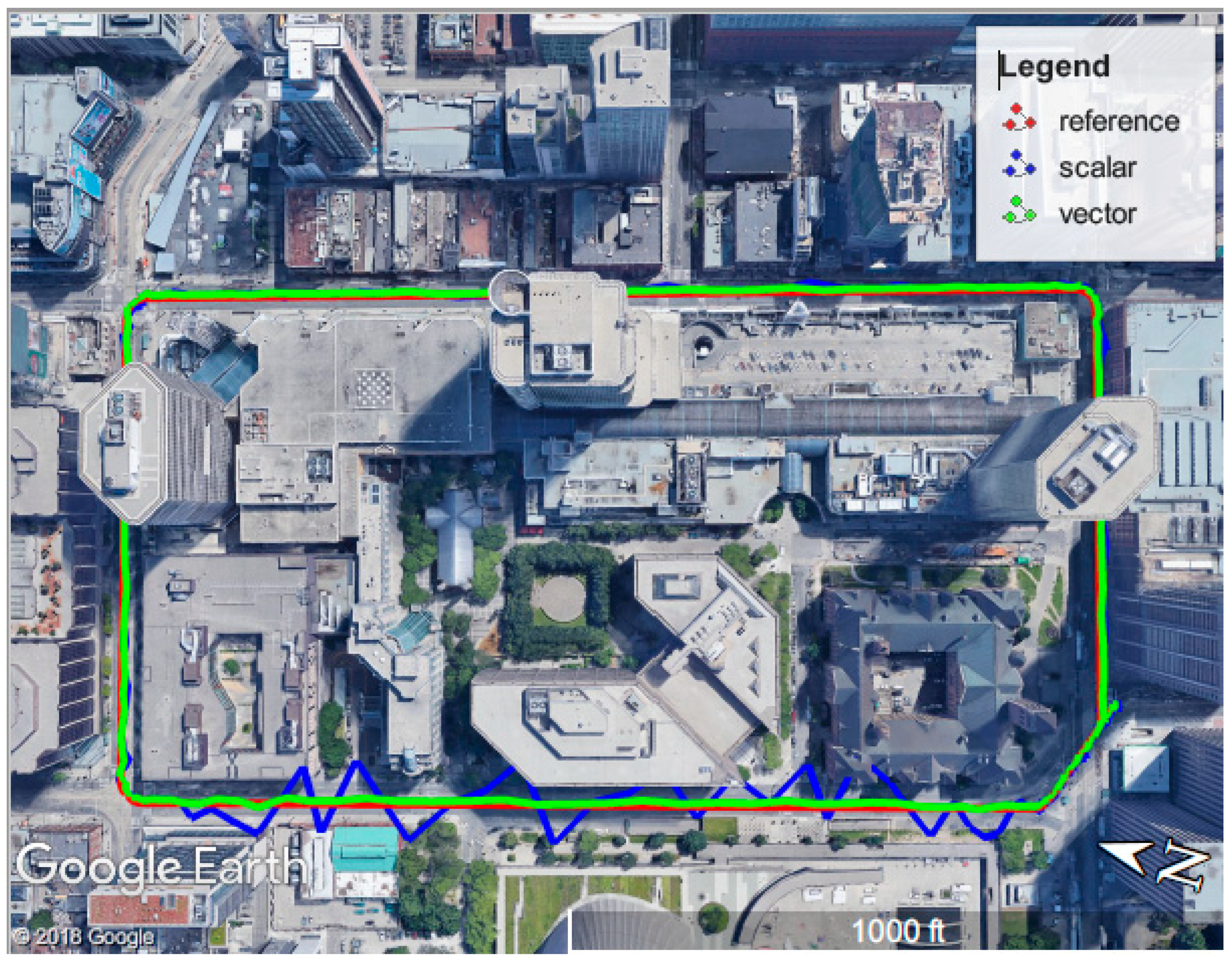
7.2. Dynamic Scenario

The details of the static antenna scenario are as follows:
  • Time of simulation: 16 January 2019 at 12:00:00 p.m.
  • Location: Downtown Toronto, ON, Canada with a starting point at 43°39′6.63″ N latitude and 79°22′54.17″ W longitude.
  • The number of visible GPS satellites: 11, as shown in Figure 6.
  • Duration: 4 min.
  • Platform: Land vehicle.

8. Results and Discussion

This section compares the performance of the vector-based SDR with its counterpart scalar-based SDR in degraded signal environments, including attenuation of the signal strength of one or more satellites, and the presence of the jamming signal. Both static and dynamic scenarios were considered. The first three scenarios are based on the static scenario described in the Section 7, while the last scenario was based on the dynamic scenario. The performance is evaluated in terms of signal tracking and navigation solution accuracy. Despite the availability of eleven visible in both static and dynamic scenarios, the number of tracked satellites inside the SDR was set to eight to assess the performance in case of the availability of fewer satellites. The selected satellites to be tracked were the ones with the highest acquisition metric, which is defined as the ratio between the first-highest peak to the second-highest peak in the acquisition search space.

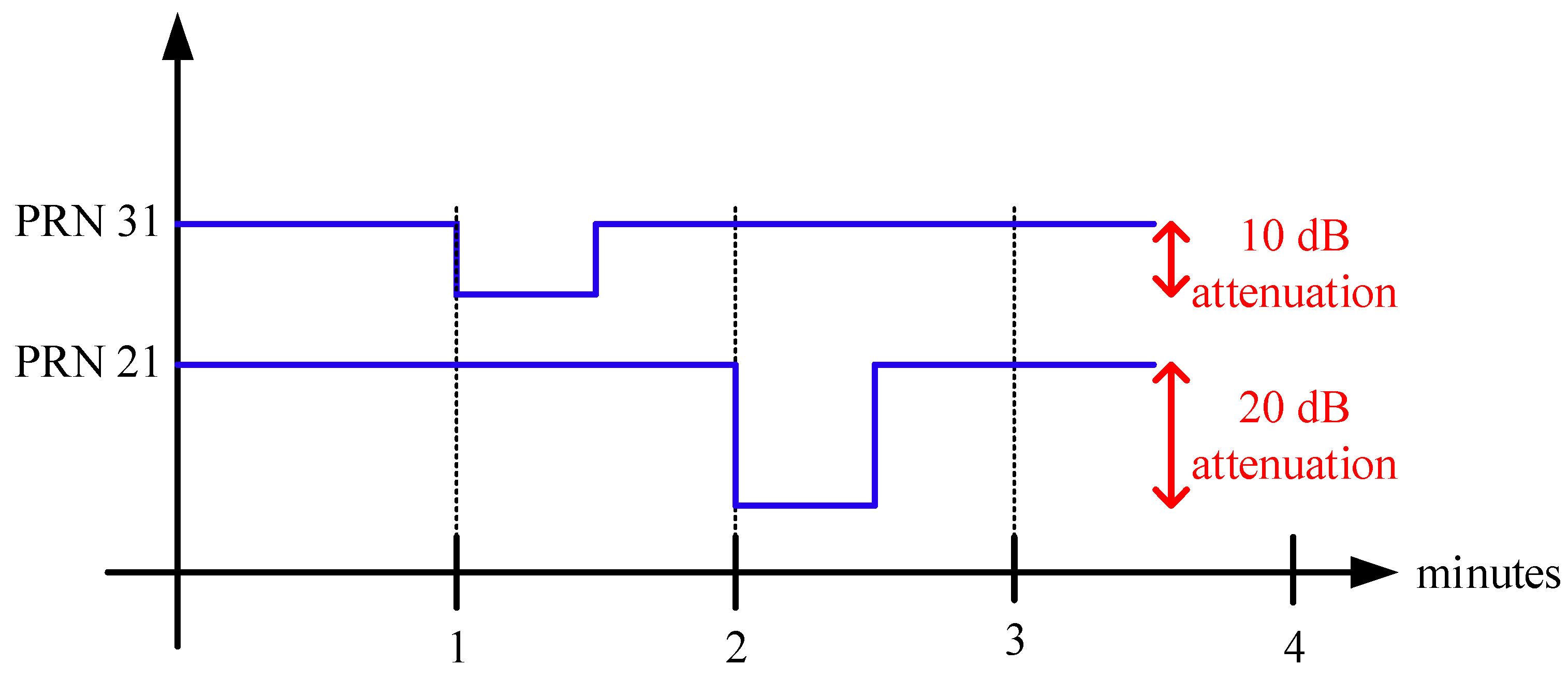
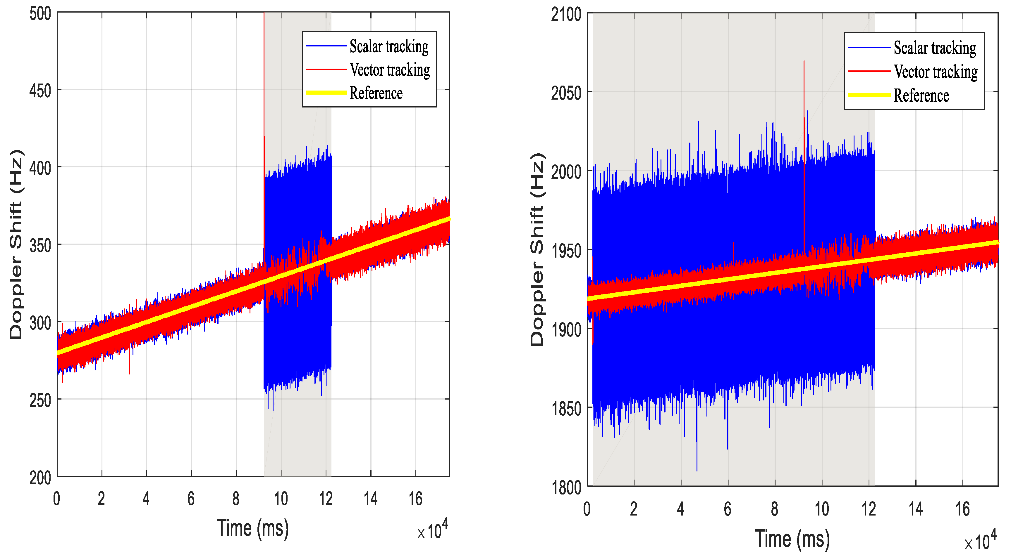
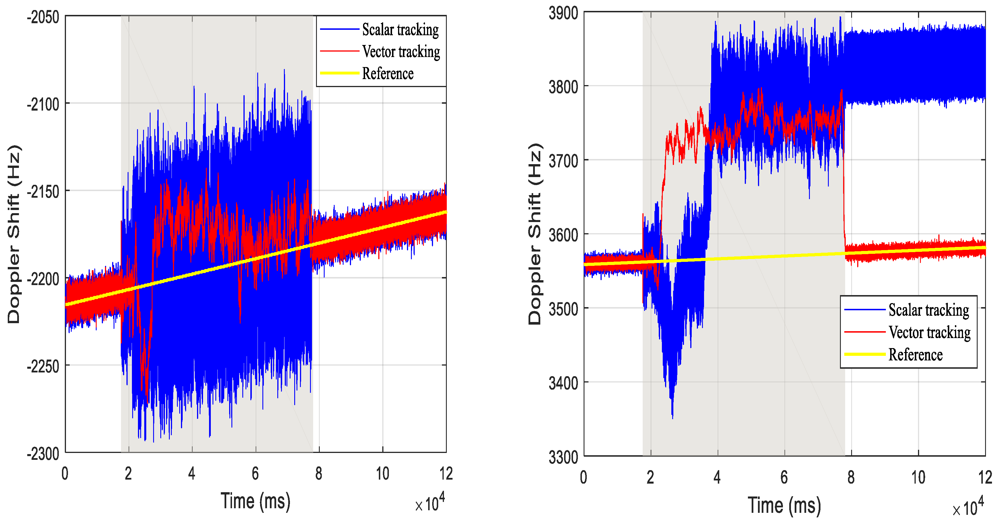
8.1. Static Scenario #1

The duration of the trajectory is 4 min. After 1 min from the start of the scenario, the signal power level of PRN 31 was attenuated by 10 dB for thirty seconds. Thirty seconds later, the signal power level of PRN 21 was attenuated by 20 dB for thirty seconds, as shown in Figure 7.
Figure 8 shows the estimated Doppler frequency from the ST and VT modules versus the reference. The shaded area in the figure denotes the period of power attenuation. ST was able to maintain the lock on the carrier frequency of PRN 31. However, the estimated Doppler frequency was noisier when compared to VT. On the contrary, ST lost track of the carrier frequency of PRN 21 during the power attenuation and failed to re-lock into the signal after the signal level returned to its normal value.
In contrast, VT was able to maintain lock-on the signal throughout the whole scenario. Table 4 shows the root mean square error (RMSE) values of the positioning solution during the duration of power attenuation. As depicted from the table, vector-based receiver outperformed scalar-based receiver in terms of positioning accuracy. The loss of carrier frequency tracking of PRN 21 in the ST loop is reflected in an erroneous position and velocity solution. In contrast, the vector-based receiver was able to provide a good navigation solution even at a signal attenuation level of 20 dB.

8.2. Static Scenario #2

The duration of the trajectory is 4 min. As shown in Figure 9, after 1 min from the start of the scenario, the signal power level of PRN 29 was attenuated by 15 dB. Afterwards, every thirty seconds, another satellite’s signal power level was attenuated by 15 dB until the number of attenuated satellites reached 4. Eventually, after thirty more seconds from the attenuation of the last satellite, all power levels were set back to their original values.
Examining Figure 10, both ST and VT loops were kept locked on to the carrier frequency of the signal during the attenuation period of all attenuated PRNs. However, the estimated Doppler frequency by ST loops was noisier compared to VT. This was translated into a better positioning accuracy, as obvious from Table 5. The table shows that the position error of the vector-based receiver is 72% better than that of a scalar-based receiver.
The outlier in the Doppler shift estimate in VT that appears in Figure 10 occurred at the instant of attenuating the signal power level of PRN 21. Nevertheless, VT was able to rapidly diverge to provide better estimates of the Doppler frequency compared to ST.

8.3. Static Scenario #3

The duration of the scenario is 3 min. In this scenario, a swept continuous wave (SCW) jamming signal is injected after 1 min from the start of the scenario and lasted for 1 min. The jamming signal parameters are summarized in Table 6.
In the next figures, the shaded area represents the duration at which the jamming signal was enabled. Figure 11 shows that both ST and VT loops failed to track the carrier frequency of the satellites throughout the jamming duration. However, the vector-based receiver was able to rapidly re-lock on the signal after disabling the jamming signal without the need to go into re-acquisition mode. On the contrary, the scalar-based receiver failed to lock to the signal after the loss of some satellites such as PRN 30. Consequently, the scalar-based receiver had to go into re-acquisition mode, which is computationally intensive compared to tracking. Figure 12 shows huge errors in the velocity solution encountered by the scalar-based receiver due to its inability to re-lock to the signal.

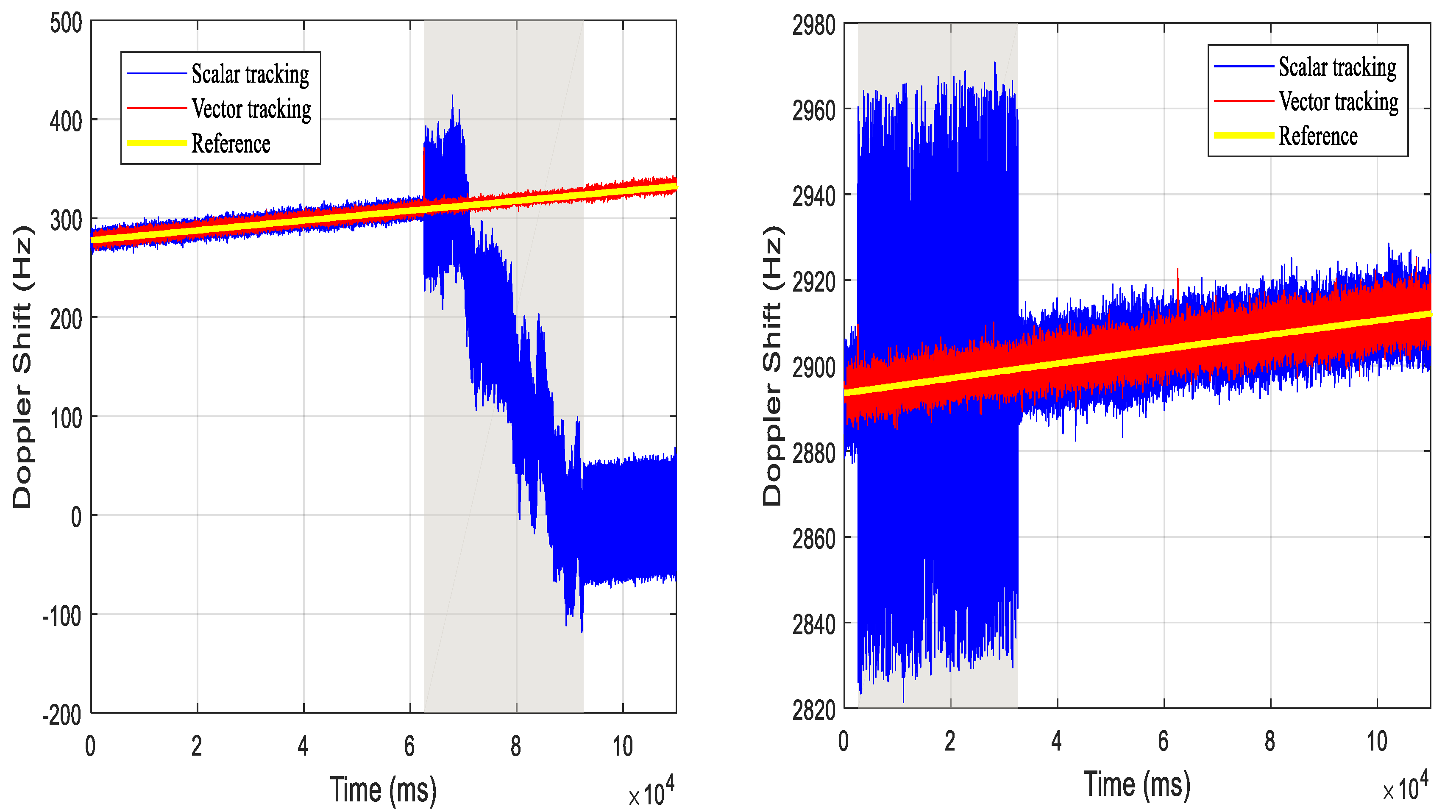
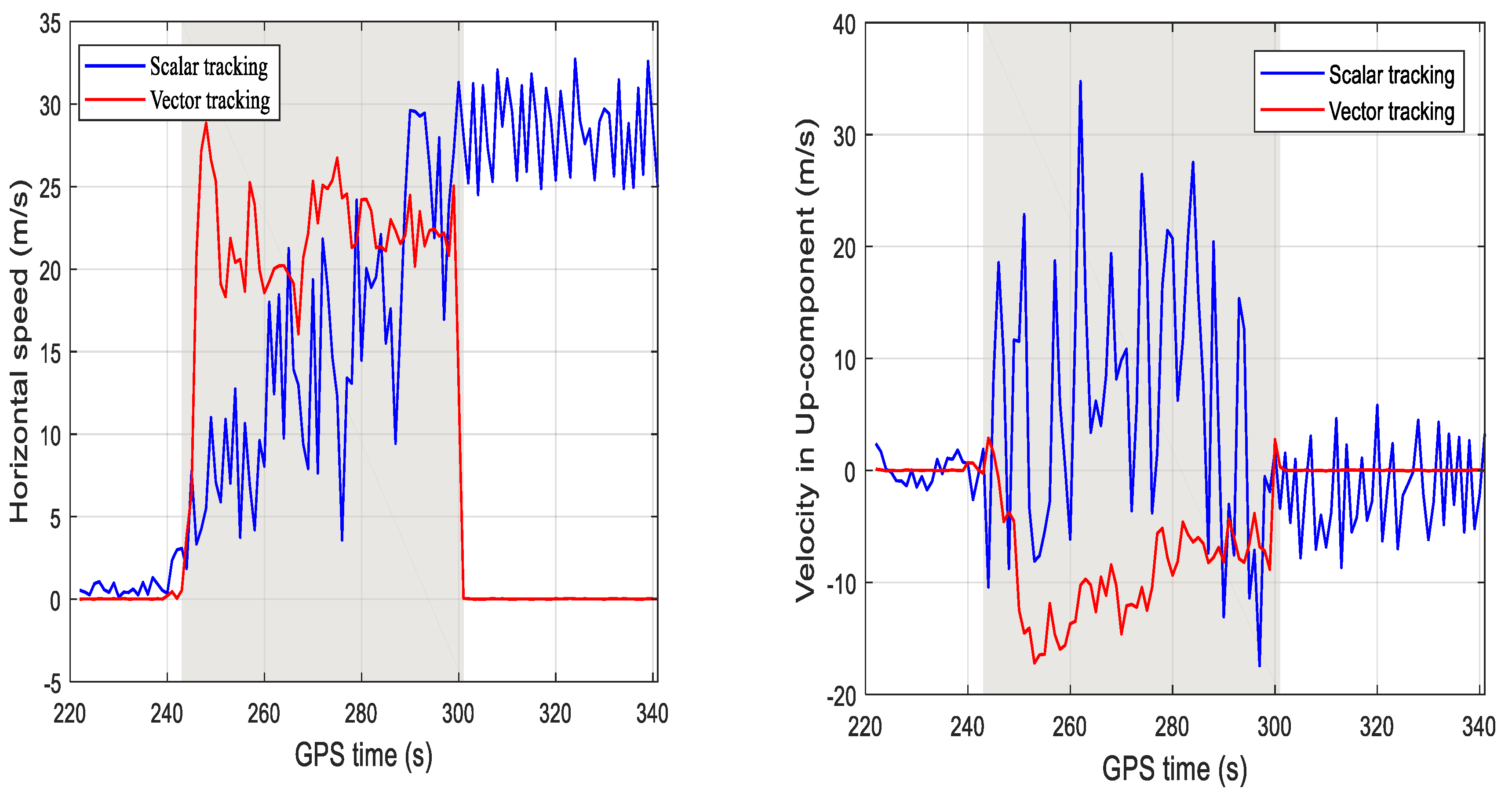
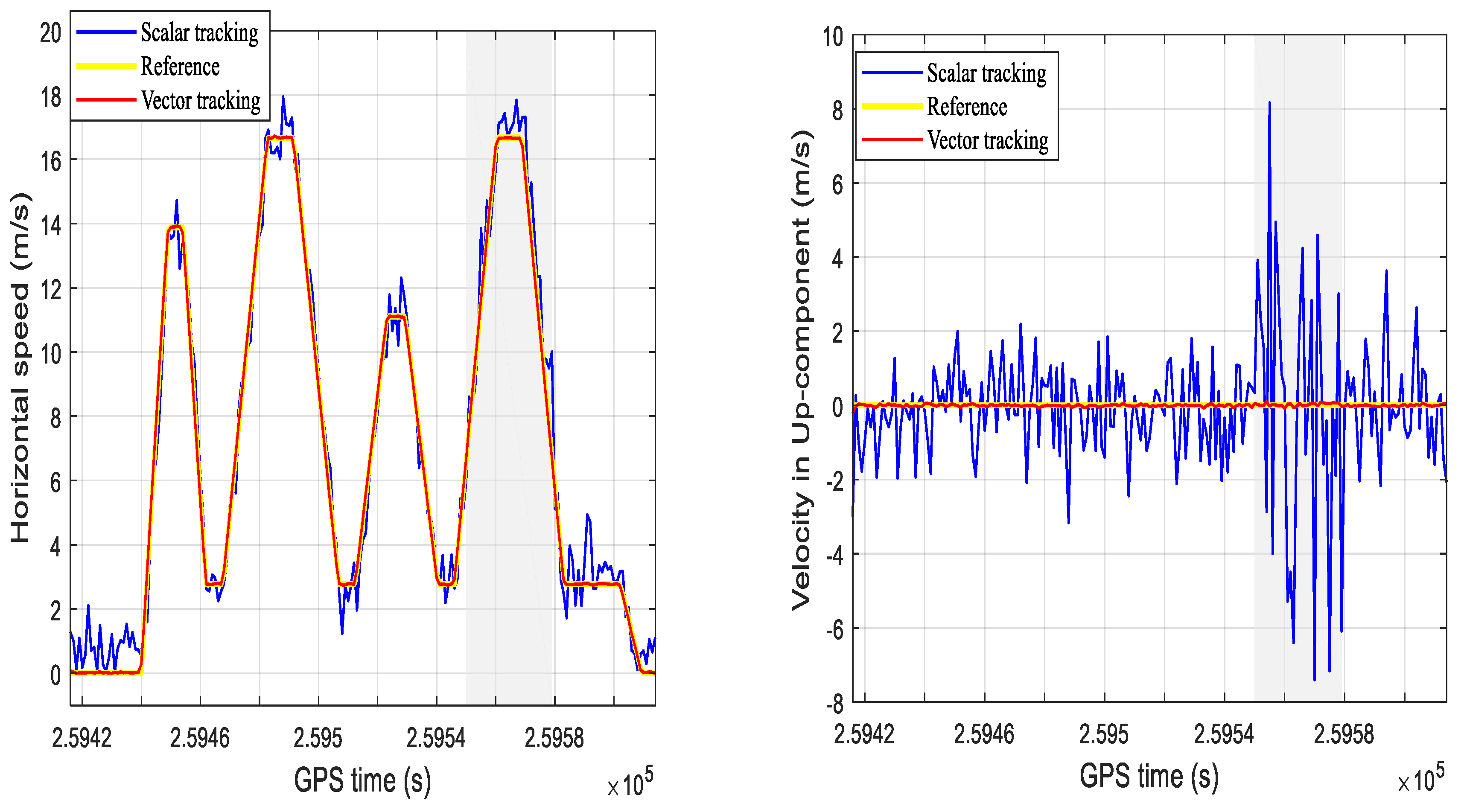
8.4. Dynamic Scenario

This trajectory simulates a land vehicle driving in downtown Toronto, incorporating a realistic driving manner such as deceleration during sharp turns. The trajectory started with the land vehicle being stationary for 1 min. Then, it accelerated to reach a final speed of 50 km/h. The land vehicle continued its motion for about 4 min with several accelerations, decelerations, and sharp turns. Eventually, it decelerated to 0 km/h to arrive at the same start point of the trajectory. The speed of the land vehicle was varied from 0 to 60 km/h throughout the trajectory. After the land vehicle started moving, by about 3 min, the signal power level of PRN 1 was attenuated by 15 dB for thirty seconds.
Figure 13 shows the navigation solution of the scalar and vector-based receivers compared to the reference visualized on Google Earth. The figure illustrates that the vector-based receiver maintained an outstanding navigation solution, despite the attenuated satellite. In contrast, the scalar-based receiver reported multiple aberrant position solutions during the period at which the satellite was attenuated. Such fluctuations in the navigation solution can lead to significant consequences in driverless vehicles. Similarly, Figure 14 shows that the velocity estimate of the vector-based receiver was more accurate compared to those of the scalar-based receiver, especially during the time interval at which PRN 1 was attenuated (shaded area in the figure). The numerical RMSE values of the positioning solution are presented in Table 7.

9. Conclusions

In this paper, an overview of vector tracking loop architectures has been presented. The performance of the vector-based receiver was compared to its counterpart scalar-based receiver in harsh signal conditions. The evaluation was based on several static and dynamic scenarios that included the attenuation of the signal power level by one with up to four satellites with various attenuation levels ranging from 10 to 20 dB. The advantages of VT loops were validated and verified as VT loops showed a better performance compared to ST loops, which tend to lose lock rapidly, due to sudden drops in the received signal power. Moreover, VT loops were effectively able to bridge a momentary outage of some attenuated satellites and keep their tracking at numerous attenuation levels, sustaining a superior position and velocity accuracy.
On the other hand, ST loops failed to track satellites attenuated by 20 dB, which result in enormous errors in the positioning solution. This is intuitively understandable, as in the vector-based receiver, the prediction of weaker signals is based on more reliable signals from other satellites. However, ST loops process the measurements coming from each channel independently.
The performance of VT and ST loops was also assessed in the presence of a jamming signal. Even though both architectures were prone to losing lock of satellites, the VT loops were able to rapidly re-track signals after the jamming signal was disabled, as contrasted with the ST loops that were unable to re-track lost signals without going into re-acquisition mode. Therefore, VT loops reduced the computational load associated with the re-acquisition of the signals. Consequently, the VT-based GNSS receiver is more suitable for augmentation with other navigation sensors for more robust and reliable positioning and navigation.
Based on the findings and conclusions of this paper, the following recommendations are suggested for future works: the performance of vector tracking loops has been assessed for a GPS L1 C/A signal; however, it can be tested on other GNSS signals. Moreover, the performance of the vector-based receiver augmented with other navigation sensors such as inertial navigation sensors (INS) could be assessed in challenging environments. Furthermore, the integration of the vector-based receiver with a jamming mitigation module could enhance the overall system’s performance in the presence of jamming.

Author Contributions

H.Y.F.E. proposed the idea, conceived and designed the simulations, analyzed the data, and wrote the paper. M.T. and A.N. reviewed the paper and simulation results. All authors have read and agreed to the published version of the manuscript.

Funding

This research received no external funding.

Conflicts of Interest

The authors declare no conflict of interest.

References

  1. Marcus, M. Growing consumer interest in jamming: Spectrum policy implications [Spectrum Policy and Regulatory Issues]. IEEE Wirel. Commun. 2014, 21, 4. [Google Scholar] [CrossRef]
  2. Elghamrawy, H.; Karaim, M.; Tamazin, M.; Noureldin, A. Experimental Evaluation of the Impact of Different Types of Jamming Signals on Commercial GNSS Receivers. Appl. Sci. 2020, 10, 4240. [Google Scholar] [CrossRef]
  3. Kuusniemi, H.; Airos, E.; Bhuiyan, M.Z.H.; Kroger, T. GNSS jammers: How vulnerable are consumer grade satellite navigation receivers? Eur. J. Navig. 2012, 10, 14–21. [Google Scholar]
  4. Tamazin, M. High Resolution Signal Processing Techniques for Enhancing GPS Receiver Performance; Queen’s University: Kingston, ON, Canada, 2015. [Google Scholar]
  5. Hsu, L.T. Integration of vector tracking loop and multipath mitigation technique and its assessment. In Proceedings of the 26th International Technical Meeting of the Satellite Division of the Institute of Navigation (ION GNSS+ 2013), Nashville, TN, USA, 16–20 September 2013; pp. 3263–3278. [Google Scholar]
  6. Hsu, L.T.; Groves, P.; Jan, S.S. Assessment of the multipath mitigation effect of vector tracking in an urban environment. In Proceedings of the ION 2013 Pacific PNT Meeting, Honolulu, HI, USA, 23–25 April 2013; pp. 498–509. [Google Scholar]
  7. Kim, K.-H.; Jee, G.-I.; Im, S.-H. Adaptive vector-tracking loop for low-quality GPS signals. Int. J. Control Autom. Syst. 2011, 9, 709–715. [Google Scholar] [CrossRef]
  8. Pany, T.; Eissfeller, B. Use of a Vector Delay Lock Loop Receiver for GNSS Signal Power Analysis in Bad Signal Conditions. In Proceedings of the IEEE/ION Position, Location, and Navigation Symposium, Coronado, CA, USA, 25–27 April 2006; pp. 893–903. [Google Scholar]
  9. Sousa, F.M.G.; Nunes, F.D. Performance comparison of a VDFLL versus VDLL and scalar GNSS receiver architectures in harsh scenarios. In Proceedings of the 2014 7th ESA Workshop on Satellite Navigation Technologies and European Workshop on GNSS Signals and Signal Processing (NAVITEC), Noordwijk, The Netherlands, 3 December 2014; pp. 1–8. [Google Scholar]
  10. Lin, T.; Abdizadeh, M.; Broumandan, A.; Wang, D.; O’Keefe, K.; Lachapelle, G. Interference suppression for high precision navigation using vector-based GNSS software receivers. In Proceedings of the 24th International Technical Meeting of the Satellite Division of The Institute of Navigation, Portland, OR, USA, 20–23 September 2011; pp. 372–383. [Google Scholar]
  11. Ko, S.J.; Eissfeller, B.; Won, J.H.; Pany, T. Assessment of vector-trackingloop performance under radio frequency interference environments. In Proceedings of the 25th International Technical Meeting of the Satellite Division of The Institute of Navigation (ION GNSS 2012), Nashville, TN, USA, 17–21 September 2012; pp. 2333–2341. [Google Scholar]
  12. Lashley, M.; Bevly, D.M. Comparison in the performance of the vector delay/frequency lock loop and equivalent scalar tracking loops in dense foliage and urban canyon. In Proceedings of the 24th International Technical Meeting of the Satellite Division of The Institute of Navigation (ION GNSS 2011), Portland, OR, USA, 20–23 September 2011; pp. 1786–1803. [Google Scholar]
  13. Borre, K.; Kudryavtsev, I. Software Defined GNSS Receiver. Procedia Eng. 2015, 104, 9–14. [Google Scholar] [CrossRef] [Green Version]
  14. Lashely, M. Modeling and Performance Analysis of GPS Vector Tracking Algorithms; Auburn University: Auburn, AL, USA, 2009. [Google Scholar]
  15. Bhattacharyya, S. Performance and Integrity Analysis of the Vector Tracking Architecture of GNSS Receivers; University of Minnesota: Minneapolis, MN, USA, 2012. [Google Scholar]
  16. Elghamrawy, H. Narrowband jamming mitigation in vector-based GPS software defined receiver. Ph.D. Thesis, Queen’s University, Kingston, ON, Canada, 2019. [Google Scholar]
  17. Krasovski, S. Vector-Based and Ultra-Tight GPS/INS Receiver Performance in the Presence of Continuous Wave Jamming; University of Calgary: Calgary, AB, USA, 2015. [Google Scholar]
  18. Li, Q.; Han, Z.; Wang, W.; Wang, X.; Xu, D. Anti-jamming scheme for GPS receiver with vector tracking loop and blind beamformer. Electron. Lett. 2014, 50, 1386–1388. [Google Scholar] [CrossRef]
  19. Petovello, M.G.; Lachapelle, G. Comparison of vector-based software receiver implementations with application to ultra-tight GPS/INS integration. In Proceedings of the 19th International Technical Meeting of the Satellite Division of The Institute of Navigation (ION GNSS 2006), Fort Worth, TX, USA, 26–29 September 2006; pp. 1790–1799. [Google Scholar]
  20. Zhao, S.; Akos, D. An open source GPS/GNSS vector tracking loop implementation, filter tuning, and results. In Proceedings of the International Technical Meeting of The Institute of Navigation, San Diego, CA, USA, 28–31 January 2019; pp. 1293–1305. [Google Scholar]
  21. Spirent. Hardware and Software User Manual for Spirent’s GSS6700 Satellite Navigation Simulation Signal Generator; Spirent: Crowley, UK, 2010. [Google Scholar]
  22. Spirent. SimGEN Software Suite for Spirent Gnss Constellation Simulation Systems; Spirent: Crowley, UK, 2018. [Google Scholar]
  23. Spirent. User Manual for the Interference Simulation System Using SimGEN, Software for the Spirent Range of Satellite Navigation Simulator Products; Spirent: Crowley, UK, 2014. [Google Scholar]
  24. NovAtel. Digital GNSS Antenna (Prototype)-DGA NovAtel R&D Project: FireHose, Test Setup and Interface Guide D1708; NovAtel Inc.: Calgary, AB, Canada, 2013. [Google Scholar]
Figure 1. Software-defined receiver (SDR) architecture.
Signals 01 00007 g001
Figure 2. Scalar tracking receiver. Scalar tracking architecture (top) and scalar tracking loop (bottom).
Signals 01 00007 g002
Figure 3. Vector tracking loop architectures. Vector delay lock loop (VDLL) (top-left), vector frequency lock loop (VFLL) (top-right), and vector delay frequency lock loop (VDFLL) (bottom).
Signals 01 00007 g003
Figure 4. Flowchart of vector tracking architecture.
Signals 01 00007 g004
Figure 5. Hardware experimental setup.
Signals 01 00007 g005
Figure 6. Sky plot. Static scenario (left) and dynamic scenario (right).
Signals 01 00007 g006
Figure 7. The signal power level for scenario #1.
Signals 01 00007 g007
Figure 8. Doppler shift for scenario #1. PRN 21 (left), and PRN 31 (right).
Signals 01 00007 g008
Figure 9. The signal power level for scenario #2.
Signals 01 00007 g009
Figure 10. Doppler shift for scenario #2. PRN 21 (left), and PRN 29 (right).
Signals 01 00007 g010
Figure 11. Doppler shift for scenario #3. PRN 16 (left), and PRN 30 (right).
Signals 01 00007 g011
Figure 12. Velocity solution for scenario #3. Horizontal speed (left), and up-velocity component (right).
Signals 01 00007 g012
Figure 13. Dynamic trajectory visualized on Google Earth.
Signals 01 00007 g013
Figure 14. Velocity solution for dynamic scenario. Horizontal speed (left), and up-velocity component (right).
Signals 01 00007 g014
Table 1. SpirentTM system simulation parameters.
ParameterValueUnit
Simulated SignalGPS L1 C/A code
Noise Floor−130dBm
Code Length1023chip
Code Frequency1.023MHz
Signal Bandwidth2.046MHz
Table 2. NovAtel FireHose parameters.
ParameterValueUnit
Intermediate Frequency (IF)0Hz
Sampling Frequency10MHz
Quantization Bits4bits
Table 3. Software receiver parameters.
ParameterValueUnit
Acquisition Search Space14kHz
Coherent Integration Time5ms
Non-Coherent Integration3blocks
Acquisition Threshold2.5
PLL Damping Ratio0.7
PLL Noise Bandwidth25Hz
DLL Damping Ratio0.7
DLL Noise Bandwidth2Hz
DLL Correlator Spacing0.5chip
Table 4. Root mean square error (RMSE) values for scenario #1.
AttenuationScaler TrackingVector Tracking
10 dB20 dB10 dB20 dB
Horizontal Position (m)4.8233.062.42.51
Horizontal Speed (m/s)1.5815.460.030.05
Up Velocity Component (m/s)1.8959.380.040.21
Table 5. RMSE values of scenario #2.
ParameterScalar TrackingVector Tracking
Horizontal Position (m)12.53.39
Horizontal Speed (m/s)50.15
Up Velocity Component (m/s)6.130.49
Table 6. Jamming signal parameters.
ParameterValue
Jamming Signal TypeSwept continuous wave
Jamming-to-Signal Ratio45 dB
Start Frequency1575.43 MHz
End Frequency1575.55 MHz
Number of Frequency Hops12
Dwell Time1 ms
Table 7. RMSE values for the dynamic scenario.
ParameterScalar TrackingVector Tracking
Horizontal Position (m)6.31.9
Horizontal Speed (m/s)1.120.12
Up Velocity Component (m/s)3.880.05

