Article

Underwater Target Recognition with Fusion of Multi-Domain Temporal Features

1
Xi’an Precision Machinery Research Institute, Xi’an 710077, China
2
School of Marine Science and Technology, Northwestern Polytechnical University, Xi’an 710072, China
*
Author to whom correspondence should be addressed.
Acoustics 2026, 8(2), 22; https://doi.org/10.3390/acoustics8020022
Submission received: 9 January 2026 / Revised: 19 March 2026 / Accepted: 23 March 2026 / Published: 25 March 2026

Abstract

The dynamic nature of acoustic environments—particularly the fluctuation of underwater channels and time-varying target observation angles—poses significant challenges for active sonar target recognition, a problem further aggravated by the scarcity of labeled training samples. To address these limitations, this paper proposes a novel recognition method enabling deep fusion of multi-domain temporal features extracted from target echoes. First, complementary features are extracted across spatial, time–frequency, and Doppler domains to achieve a comprehensive and discriminative representation of targets. Subsequently, we introduce a feature vector-level fusion mechanism designed specifically for few-shot learning, integrating a meta-knowledge-driven multi-stream feature extractor with an internal memory module within the feature tensor framework. This architecture constitutes the Multi-domain Temporal Feature Fusion Recognition Network (MTFF-RNet). The proposed approach is evaluated on a hybrid dataset combining simulated and experimental data, achieving a high recognition accuracy of 96.2% for both targets and interferents. Experimental results demonstrate that MTFF-RNet significantly enhances robustness and adaptability under varying underwater acoustic conditions and dynamic viewing geometries.

1. Introduction

Active sonar target recognition (ASTR) plays a crucial role in marine information acquisition, with broad applications in underwater surveillance, navigation, and environmental monitoring [1,2,3,4]. However, the underwater acoustic channel exhibits pronounced time-varying and space-varying characteristics due to the complex interplay of multiple factors, including sound speed gradients, boundary reflections, ambient noise, and anthropogenic interference [5,6]. Moreover, underwater targets—particularly mobile ones—typically possess streamlined geometries, leading to aspect-dependent scattering behaviors that further complicate recognition tasks [7]. Consequently, channel-induced signal fluctuations and continuous variations in target aspect angles represent two major sources of uncertainty that significantly degrade ASTR performance.
To address these issues, conventional methods have employed multi-parameter joint estimation to enhance algorithmic robustness [8,9]. In recent years, deep learning has emerged as a promising alternative, offering powerful feature representation capabilities for ASTR. However, practical deployment remains hindered by the scarcity of labeled training data, which stems from the high cost of data collection, the diversity of target types and interference sources, and the inherent variability of underwater environments. As a result, the few-shot learning problem has become a critical bottleneck in developing reliable ASTR systems. To mitigate this limitation, recent efforts focusing on few-shot learning strategies combined with multi-feature fusion frameworks have demonstrated notable progress.
A feedforward neural network utilizing power spectrum statistics, LPC coefficients, and AR coefficients achieved over 90% classification accuracy on a six-class target dataset collected in a controlled pool environment [10]. To distinguish real targets from clutter, a CNN-based approach employing fused azimuth-time spectra and spectrograms was validated using sea trial data, confirming its practical applicability [11]. Another fusion method integrating MFCC, spectrograms, WVD, CWT, and spatial spectra through the RS-LFMD convolutional network attained an 87% accuracy rate in identifying targets embedded in oceanic clutter [12,13]. Further improvements were achieved by LTFSD-Net and an attention-enhanced convolutional network, which jointly exploited time-domain waveforms, Mel spectra, spectrograms, and CWT spectra to classify three types of underwater targets, yielding an accuracy of 84.36% on static test datasets from the South China Sea [14,15]. An enhanced ConvNeXt-V2 architecture, termed ConvNeXt-DCA, fused spectrograms, SPWVD, and CWT features extracted from left, middle, and right subarray echoes for three-target classification, achieving a 92.1% accuracy rate validated on both anechoic pool and static sea trial data [16]. The physical-informed Bayesian graph multimodal recognition method (PBGMR) integrated three complementary modalities—Fourier synchronous compressive transform (FSST), beam–time–distance (BTR), and tensor features from ConvNeXt-V2—reaching 92.31% accuracy on a four-target North Sea dataset comprising pipes, cylinders, spheres, and UUVs [17]. Moreover, a meta-learning-based framework designed domain-specific feature extraction networks according to spectral characteristics across spatial, time–frequency, and Doppler domains. This approach enabled synergistic integration of multi-domain information, and validation—including through ablation studies—on experimental data demonstrated improved perspective adaptability of the recognition algorithm [18].
By leveraging complementary multi-domain features, these aforementioned approaches have effectively enhanced the adaptability and robustness of target recognition algorithms to variations in underwater acoustic channels and target perspectives. Nevertheless, they are primarily limited to fusing multi-domain features extracted from a single burst of target echoes. Under conditions of significant channel fluctuations or large target aspect angle changes, echo signals may become unstable, leading to a notable decline in recognition performance based on single-burst features. In such scenarios, the decision-level integration of recognition results across multiple bursts becomes essential to improve the overall classification accuracy.
To address this limitation, the MotionSqueeze module and a ConvNeXt v2 classifier have been introduced to capture temporal variations in spectrograms between consecutive frames of effective echoes. The experimental results demonstrate that this method outperforms single-frame echo-based approaches in recognition performance [19]. Similarly, in [20], a pulse train consisting of 1 to 50 broadband encoded clicks is employed to collect target echoes, and a convolutional neural network is applied to classify spectral peaks and troughs. The results show that using 50 pulses achieves optimal performance in both detection and classification. These studies collectively demonstrate that exploiting multi-burst echo information helps mitigate the adverse effects of dynamic acoustic environments—such as channel instability and viewpoint variation—on recognition robustness. However, due to the inherent diversity of underwater targets, varying observation angles, and the time- and space-varying nature of underwater acoustic channels, relying solely on a single type of feature remains insufficient for robust recognition in practical applications [18].
This study aims to overcome the limitations and application constraints of existing multi-domain feature fusion and time-series-based single feature recognition algorithms, with a specific focus on enhancing active sonar target recognition performance under challenging conditions characterized by fluctuating underwater acoustic channels and dynamically varying target observation angles. To this end, we extracted multi-domain features from continuous multi-burst scattering echoes of targets, investigated effective fusion strategies for multi-domain temporal features, and developed a novel active sonar target recognition method based on multi-domain temporal feature fusion. The main contributions of this work are summarized as follows:
  • We extracted time series features of underwater target scattering in the spatial, time–frequency, and Doppler domains. These three complementary feature representations capture distinct physical characteristics of the target response, thereby providing enhanced discriminative capability. By systematically analyzing fusion strategies for multi-domain temporal features, we propose a feature vector-level (or mid-level) multi-domain temporal feature fusion mechanism specifically designed for few-shot learning scenarios.
  • We designed a meta-knowledge-driven multi-stream feature extraction network and introduced an internal memory module for multi-domain feature tensors, leading to the construction of a Multi-domain Temporal Fusion Network (MTFF-Net). This architecture enables the effective fusion of multi-domain temporal features through a pipelined processing framework, facilitating both real-time implementation and practical engineering deployment.
  • We established a comprehensive time series dataset using both simulation-generated signals and experimental data to evaluate the proposed method. The experimental results demonstrate a recognition accuracy of 96.25% for real targets and multi-source interferences, validating the robustness of the proposed approach. The results confirm that the proposed method significantly improves target recognition performance in complex environments involving channel fluctuations (e.g., interface reverberation, low signal-to-noise ratio) and time-varying target perspective.
The remainder of this paper is organized as follows: Section 2 details the technical framework of the proposed multi-domain temporal feature-based active sonar target recognition method. Section 3 presents and discusses the experimental results. Finally, Section 4 concludes the paper with a summary of the key findings and potential future directions.

2. Methods

This paper proposes a multi-domain temporal feature fusion method for underwater moving target recognition and constructs a multi-domain feature extractor along with a Multi-domain Temporal Feature Fusion Recognition Network (MTFF-RNet), thereby enhancing the environmental adaptability of active sonar target recognition, as illustrated in Figure 1. The proposed method extracts spatial-domain D3SF features, time–frequency-domain EPWVD features, and Doppler-domain DFSD features from the raw data of array elements and conventional beamforming data [21]. After evaluating four different approaches to multi-domain temporal feature fusion, the feature vector-level fusion strategy was selected to address the challenges posed by limited and imbalanced training samples. Three domain-specific classification networks were independently developed and trained to yield dedicated feature extractors for each domain. An internal memory module is introduced to store and manage multi-burst effective echo features—specifically, spatial-domain (Fs), time–frequency-domain (Ftf), and Doppler-domain (Fd) feature vectors—over time. Leveraging these pre-trained feature extractors, MTFF-RNet integrates a three-dimensional convolutional layer (Conv3D1) and a linear classification layer (Linear1). Conv3D1 and Linear1 are subsequently trained on a multi-domain temporal dataset to form the final inference network. The Conv3D layer captures high-dimensional spatiotemporal–statistical characteristics across domains and time steps, which are then fed into the linear classifier for final decision making. As a result, the proposed framework significantly improves the robustness of target recognition under challenging conditions such as underwater channel fluctuations and variations in relative motion perspective.

2.1. Extraction of Multi-Dimensional Features

The multi-domain feature extraction methods for underwater targets primarily encompass spatial spectrum estimation, time–frequency analysis, and auditory features [12,13]. Our research team has conducted an in-depth simulation analysis of the representational capabilities of spatial spectrum estimation and time–frequency analysis features, from the perspective of the coupled physical processes underlying target scattering and underwater feature extraction [22]. By comprehensively considering the homogeneity and complementarity among multi-domain features, we propose a method to extract target characteristics separately in the spatial, time–frequency, and Doppler domains. These features collectively capture distinct aspects of the target—such as its geometric contour, echo intensity distribution, and dynamic state—from complementary domain-specific perspectives.
In the spatial domain, a three-dimensional spatial feature (D3SF) is formulated by integrating the generalized MUSIC algorithm [23] with the range dimension, as defined in Equations (1) and (2).
P ( θ , ψ ) = arg min θ , ψ λ min Re Φ H ( θ , ψ ) U ^ N U ^ N H Φ ( θ , ψ )
D 3 S F ( θ , ψ , M ) = { P ( θ , ψ , m ) } m = M + M , m Z +
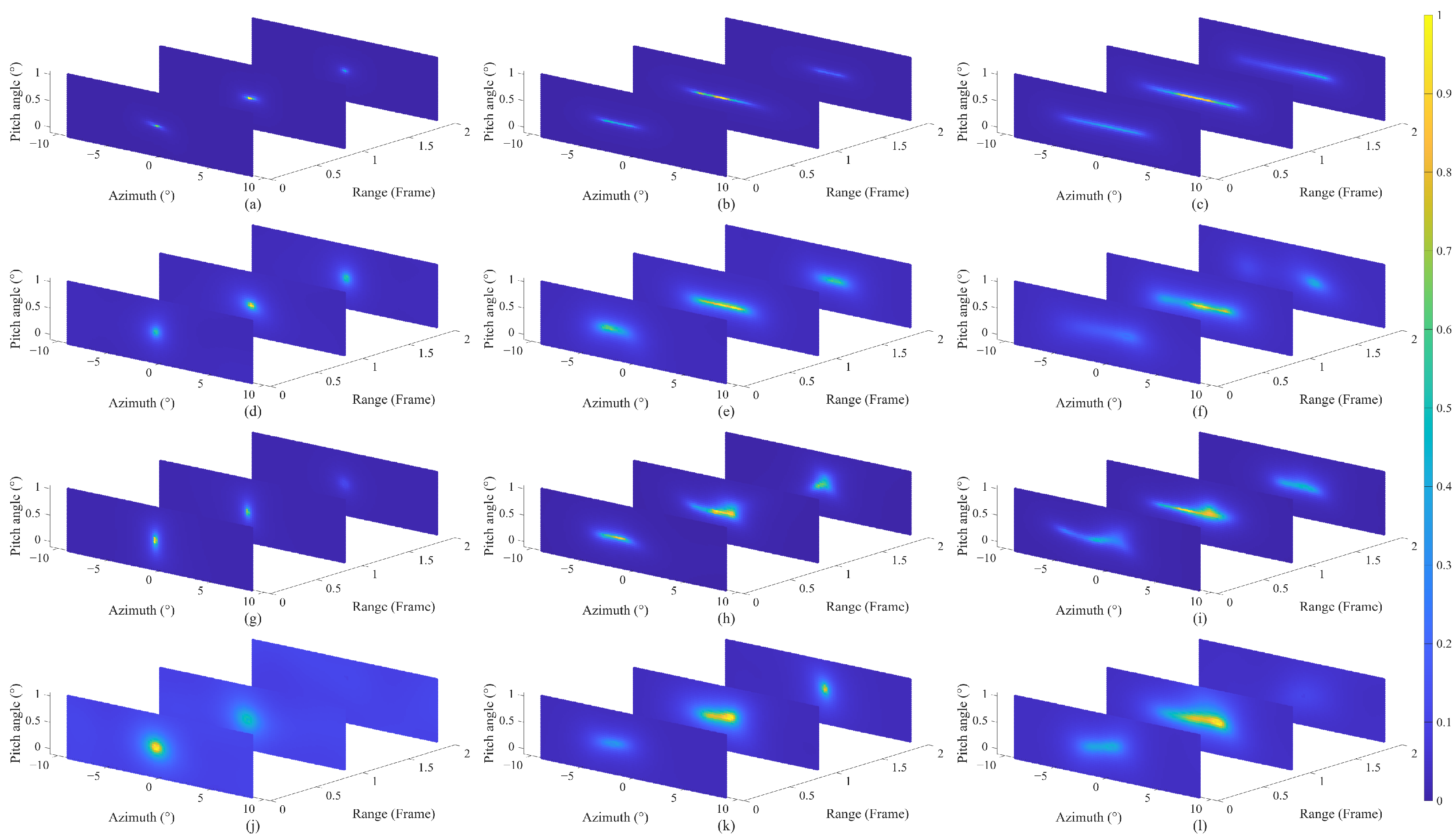
where, λmin(·) denotes the minimum eigenvalue of a matrix, and Φ(θ, ψ) is a diagonal matrix constructed from the sonar array steering vector a(θ, ψ). Here, U ^ N represents the estimated noise subspace. When m = 0, the slice corresponds to the range bin with maximum energy; m < 0 indicates a closer range slice, while m > 0 indicates a farther one. The total number of spatial spectrum slices used is 2M + 1, with M = 1 in this study. Equation (2) characterizes the energy distribution of target scattering across azimuth, pitch angle, and range dimensions. Figure 2 presents the D3SF spatial spectra of multi-source interference (MSI) and volume targets, acquired using a linear frequency-modulated (LFM) signal with a duration of 65 ms and a starting frequency of 30 kHz, under varying observation angles and signal-to-noise ratio (SNR) conditions. Owing to the shielding effect inherent in volume targets, the D3SF spatial spectrum achieves superior target resolution compared to conventional spatial spectra.
In the time–frequency domain, the enhanced pseudo Wigner–Ville distribution (EPWVD), which is derived from the pseudo Wigner–Ville distribution (PWVD) [24], is employed as defined in Equations (3) and (4) [18].
P W V D ( t , f ) = x ( t + τ 2 ) x ( t τ 2 ) h ( τ ) e j 2 π f τ d τ = W V D ( t , f ) H ( f )
E P W V D ( t , f ) = P W V D ( t , f ) δ ( r ( t , f ) ) h ( t )
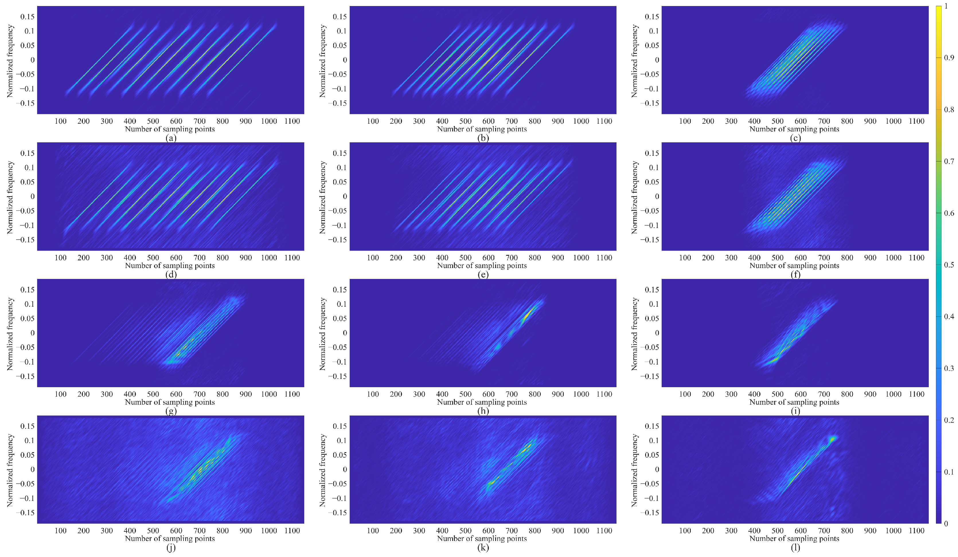
where τ denotes the time delay, t represents time, and f stands for frequency; h(τ) is the time-domain window function of the Wigner–Ville distribution (WVD) [25], and H(f) is its corresponding frequency-domain representation. With an optimized window function, the PWVD effectively suppresses cross terms while preserving strong time–frequency concentration. In Equation (4), δ(·) denotes the unit impulse function, r(t, f) represents the time–frequency characterization function of the frequency-modulated signal, and h(t) is the time-domain window function. This method applies the frequency modulation function of the active sonar transmitted signal to filter and smooth the time–frequency spectrogram, thereby enhancing the discriminative characteristics of the echo in the time–frequency domain. Let h(τ) be a Hanning window with a hop size of 96, and let h(t) be a Hamming window with a hop size of 32. Let the transmitted signal be a linear frequency-modulated (LFM) chirp signal with a duration of 65 ms and a starting frequency of 30 kHz. Figure 3 illustrates the EPWVD spectra of volume target and multi-source interference under varying observation angles and signal-to-noise ratios (SNRs). As observed in the figure, due to the streamlined structure of underwater targets, the target resolution degrades when the aspect angle approaches 90°. The simulation results demonstrate that cross terms are effectively suppressed when the acoustic path difference between two point sources exceeds 3 ms.
Doppler domain features refer to the Doppler broadening induced by the interaction of a single-frequency continuous-wave (CW) signal transmitted by active sonar with a moving target, primarily influenced by the target’s physical dimensions and geometric contour. When the volume target is modeled as a collection of finite volume elements, and the transmitted signal frequency is denoted by f0, the Doppler shift component—excluding the carrier frequency—of the volume element located at rT at time t is given by fd(f0, rT, t), and the ensemble of all such Doppler shifts forms a non-stationary random process. Under illumination by a transmitted signal of pulse duration Tb, the Doppler components of the echo from the volume target can be expressed as
D T ( f d ) = T b V T f d ( f 0 , r T , t ) d V d t
where T b denotes the effective echo duration corresponding to the transmitted pulse width Tb. The Doppler components of the N-source interference echo can be expressed as
D I ( f d ) = k = 1 N f d ( f 0 , r T , t ) = k = 1 N f d k
As can be observed from Equations (5) and (6), the Doppler components of multi-source interference and volume target echoes exhibit significant differences. The two-dimensional time-delay and frequency-shift correlation function of the echo signal, obtained after removing the fundamental frequency component, characterizes the target’s Doppler frequency shift distribution (DFSD) [18], as given in Equations (7) and (8).
F d ( τ , f d ) = s ^ t + τ 2 s ^ t τ 2 e j 2 π f d τ d t
D F S D ( τ , f d ) = F d ( τ , f d ) F d ( τ , f d )
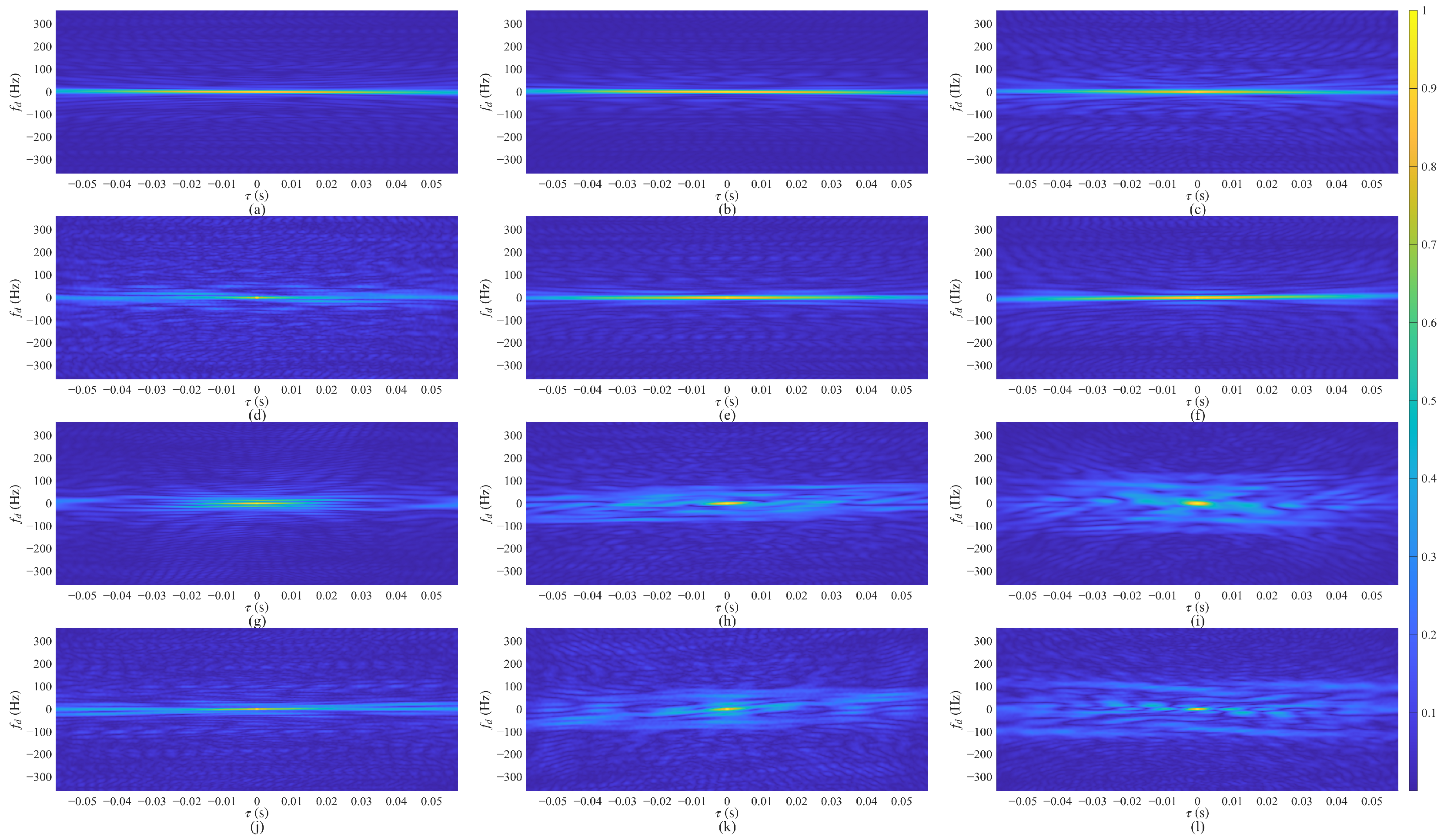
where, s ^ ( t ) denotes the estimated effective echoes. The Doppler frequency shift distribution DFSD(τ, fd) has a mathematical form analogous to the ambiguity function used in the analysis of active sonar transmitted waveforms [26]. Let the transmitted signal be a continuous-wave (CW) tone at 30 kHz with a duration of 65 ms, and let the target’s speed be 18 knots. Figure 4 presents the DFSD spectra of multi-source interference and volume targets under varying aspect angles and SNRs.

2.2. Temporal Echo Features

When the sonar platform and the target are in motion, the target’s echo characteristics exhibit time-varying and space-varying behavior, resulting in instability. In complex marine environments such as shallow water, reverberation and multi-path effects induce fluctuations in the underwater acoustic channel, which further degrade the stability of the target echo. These factors collectively reduce the robustness of multi-domain feature-based target recognition algorithms, primarily due to insufficient consideration of the temporal correlation among multi-burst echo features.
As the sonar approaches the target, sequential echo data containing multiple bursts and multiple aspect views can be acquired. Over time and across spatial dimensions, parameters such as the relative attitude, range, and relative velocity between the sonar and the target vary dynamically, while the underwater acoustic channel also experiences fluctuations. Assuming that the time-varying azimuth angle θ(t) and pitch angle ψ(t) characterize the relative orientation changes, that the channel fluctuation is modeled by C(t), the radial distance by r(t), and the relative velocity by v(t), the m-th feature of the target echo can then be expressed as
F m ( t ) = f m θ ( t ) , ψ ( t ) , C ( t ) , r ( t ) , v ( t )
The active sonar transmits pulses at a fixed pulse repetition interval (PRI), thereby acquiring the target echo sequence periodically. Consequently, Equation (9) can be reformulated as
F m ( n T s ) = f m θ ( n T s ) , ψ ( n T s ) , C ( n T s ) , r ( n T s ) , v ( n T s )
The statistical characteristics of multi-domain time-series echoes provide valuable information that enhances the robustness of target recognition. Based on the tensor stacking method [12,27], the fusion of multi-domain time-series echo features can be categorized into four distinct modes according to the stage at which integration occurs. Using the time-series feature data from the spatial, time–frequency, and Doppler domains acquired in this study as illustrative examples, the classification networks corresponding to these four fusion modes are described below.
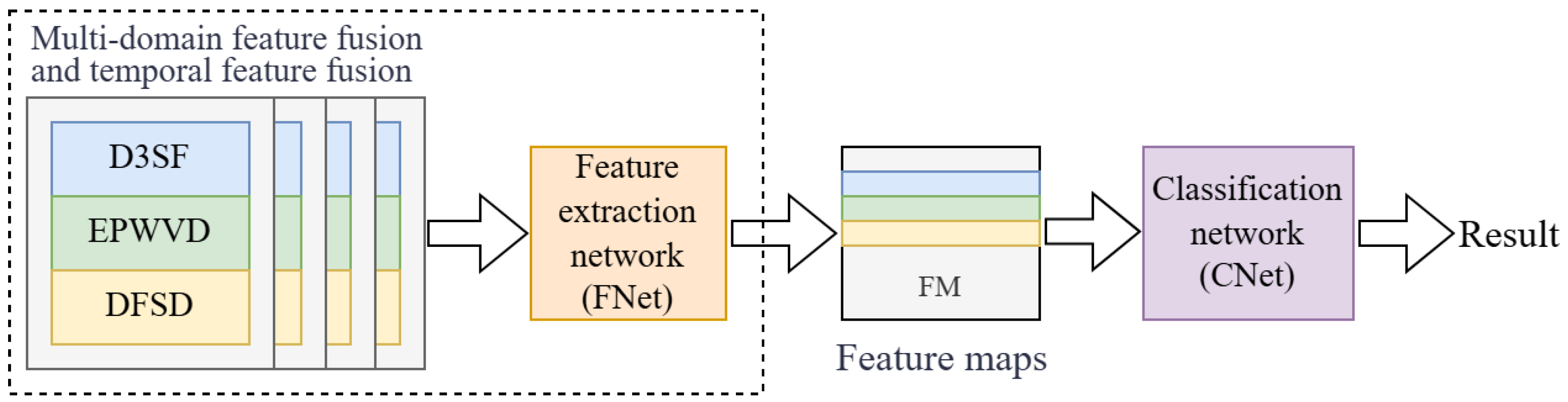
Mode 1: The multi-domain time-series feature data from four consecutive bursts are directly input to the feature extraction network, enabling concurrent integration of multi-domain and temporal features at the feature level. The resulting classification output, denoted as R1, is expressed as
R 1 = C N e t ( F N e t ( F 1 s , F 2 s , F 3 s ) )
where CNet denotes the fusion classification network, FNet denotes the feature extraction network, and F i s represents the temporal feature tensor corresponding to the i-th feature, where the superscript s indicates the inclusion of temporal dynamics. The architecture of the Mode 1 fusion network is illustrated in Figure 5.
In Figure 5, multi-domain and temporal features are fused at the feature level. The time-series feature data from the spatial, time–frequency, and Doppler domains are directly fed into the feature extraction network via dimensional expansion or tensor stacking—operations that increase either the data size or the data dimension. This enables the network to learn a unified representation that integrates both temporal dynamics and multi-domain characteristics, and the resulting feature vectors are subsequently classified by the classifier to achieve target identification.
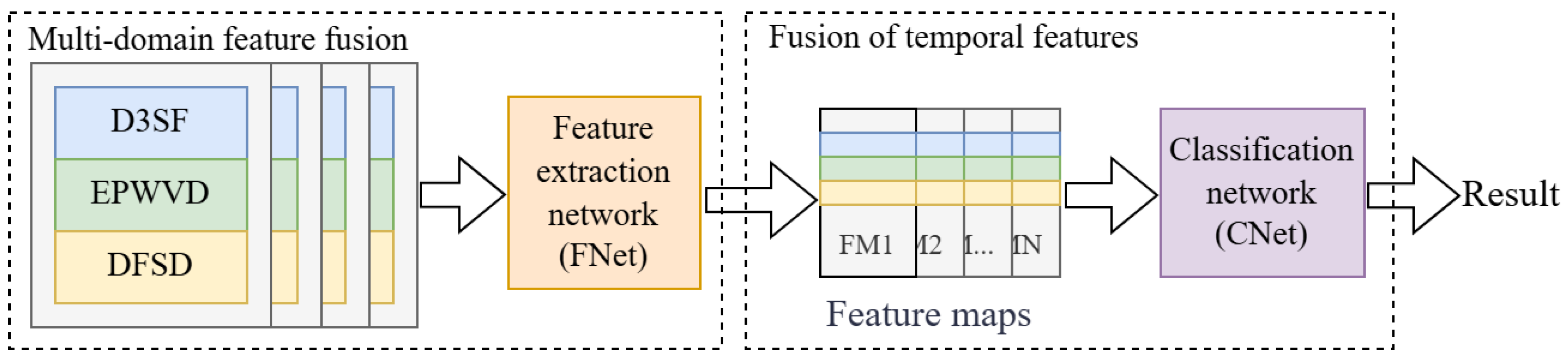
Mode 2: Multi-domain feature fusion is performed at the feature level, while temporal feature fusion is conducted at the feature vector level—corresponding to the mid-level feature stage. The resulting classification output, denoted as R2, is expressed as
R 2 = C N e t ( F T 1 , F T 2 , , F T N ) F T n = F N e t ( F 1 n , F 2 n , F 3 n )
where F 1 n , F 2 n , and F 3 n represent the two-dimensional tensors obtained by transforming the three types of feature data at the n-th burst. F T n denotes the fused 2D feature tensor of the three features at the n-th burst, and the subscript T indicates that the quantity is a feature tensor. The structural schematic of the Mode 2 fusion network is illustrated in Figure 6.
As illustrated in Figure 6, feature fusion is conducted in two stages. In the first stage, spatial, time–frequency, and Doppler domain features are fed into the feature extraction network via concatenation or stacking to generate multi-domain fused representations. In the second stage, temporal feature vectors are aggregated across multiple bursts and subsequently fed into a classifier for final target classification.
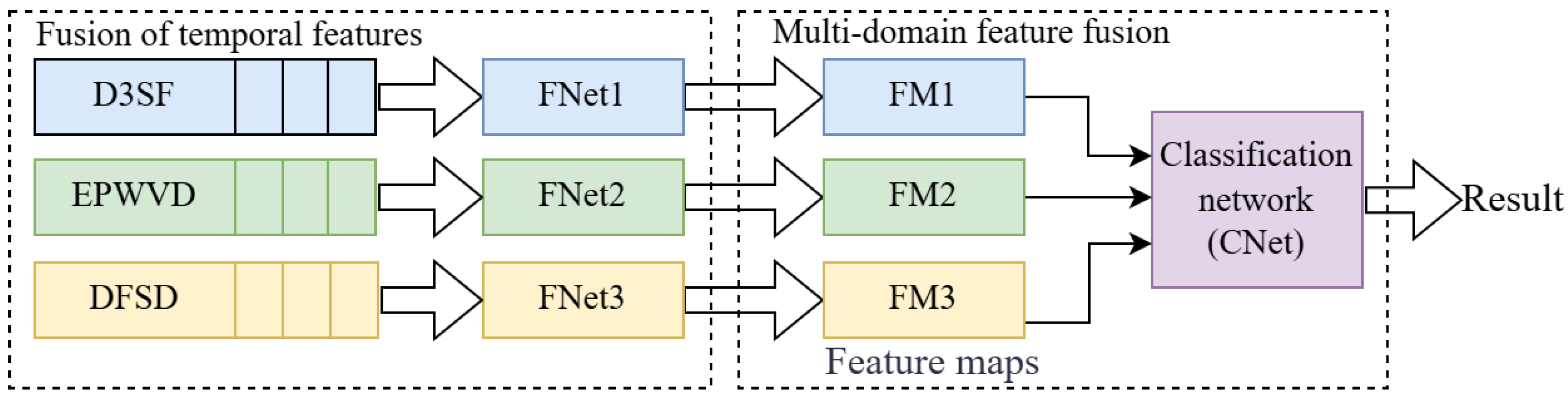
Mode 3: Temporal feature fusion is performed at the feature level, while multi-domain feature fusion is conducted at the feature vector level. The classification result, denoted as R3, is expressed as
R 3 = C N e t ( F N e t 1 ( F 1 s ) , F N e t 2 ( F 2 s ) , F N e t 3 ( F 3 s ) )
where FNeti denotes the feature extraction network for the i-th feature. The structural schematic of Mode 3 fusion network is illustrated in Figure 7.
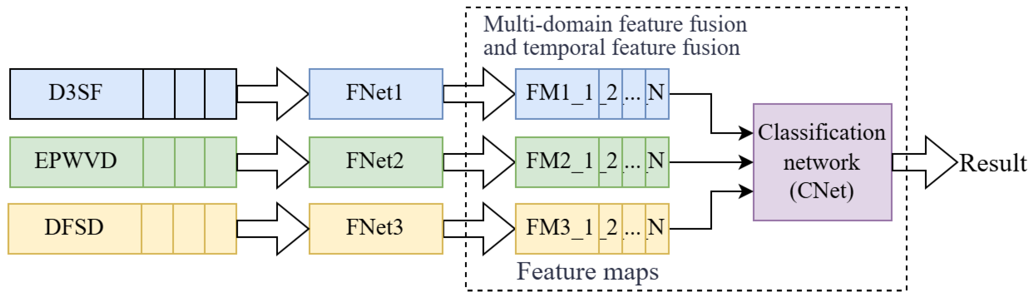
As shown in Figure 7, the feature fusion process consists of two stages. In the first stage, time-series feature sequences of individual features are fed into the feature extraction networks via stacking to generate temporal feature vectors FM1, FM2, and FM3 corresponding to the spatial, time–frequency, and Doppler domains, respectively. In the second stage, these multi-domain temporal feature vectors are integrated within the classification network to perform final target classification.
Mode 4: Multi-domain temporal feature fusion is performed at the feature vector level. The classification result, denoted as R4, is given by
R 4 = C N e t ( F m s ) F m s = s t a c k ( [ F T 1 s , F T 2 s , F T 3 s ] ) F T 1 s = { F T 1 n = F N e t 1 ( F 1 n ) , n = 1 , 2 , , N } F T 2 s = { F T 2 n = F N e t 2 ( F 2 n ) , n = 1 , 2 , , N } F T 3 s = { F T 3 n = F N e t 3 ( F 3 n ) , n = 1 , 2 , , N }
where F T 1 n , F T 2 n , and F T 3 n denote the single feature vectors (1D) of the three feature types, respectively, whereas F T 1 s , F T 2 s , and F T 3 s represent 2D tensors formed by stacking the corresponding single feature vectors over time. The 3D feature tensor F m s is constructed by concatenating F T 1 s , F T 2 s , and F T 3 s along the feature dimension. FNeti extracts feature vector level temporal features for the i-th input feature across multiple time steps. The architecture of the Mode 4 fusion network is illustrated in Figure 8.
As illustrated in Figure 8, multi-domain and temporal features are jointly fused at the feature vector level. Single-burst feature data from the spatial, time–frequency, and Doppler domains are sequentially fed into the feature extraction networks FNet1, FNet2, and FNet3, yielding the single feature, single-burst feature vectors FM1_i, FM2_i, and FM3_i. These vectors are accumulated over multiple bursts to construct a three-dimensional tensor representing multi-domain temporal features. High-level statistical characteristics are then extracted via 3D convolutional operations, followed by classification using a linear classifier to perform final target recognition.
Mode 1 simultaneously fuses multi-domain temporal feature information at the feature level, which has the highest requirement for the representation ability of the feature extraction network. Mode 4 focuses on single feature extraction at the feature level, which has the lowest requirement for the network’s representation ability and is more suitable for few-shot learning scenarios. Mode 2 and 3 fuse multi-domain feature information or temporal feature information at the feature level, and their requirements for the network’s representation ability are higher than that of Mode 4. In this study, we adopt Mode 4 to achieve the fusion of multi-domain temporal features. On the one hand, it has the lowest requirement for the representation ability of the feature extraction networks, which is most in line with the needs of few-shot learning, and the feature extraction networks can be optimized according to the characteristics of the feature spectra of each domain. On the other hand, it can fully utilize the feature extraction networks based on meta-learning and its meta-knowledge in previous research results [18], add an internal memory module and redesign the classification network to achieve the fusion of multi-domain temporal features. Mode 4 distributes the computational load, which is more conducive to the deployment of multiple AI chips in real-time applications.
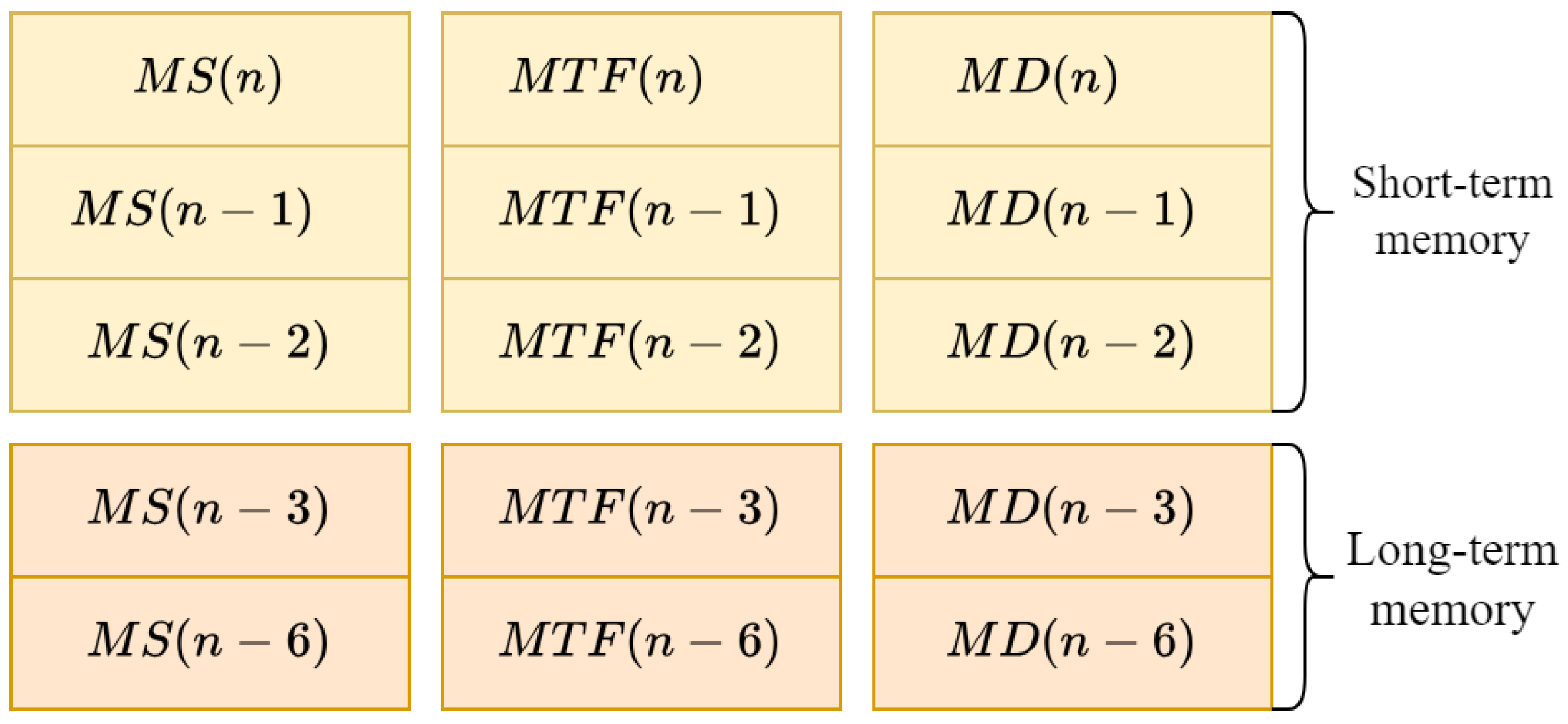
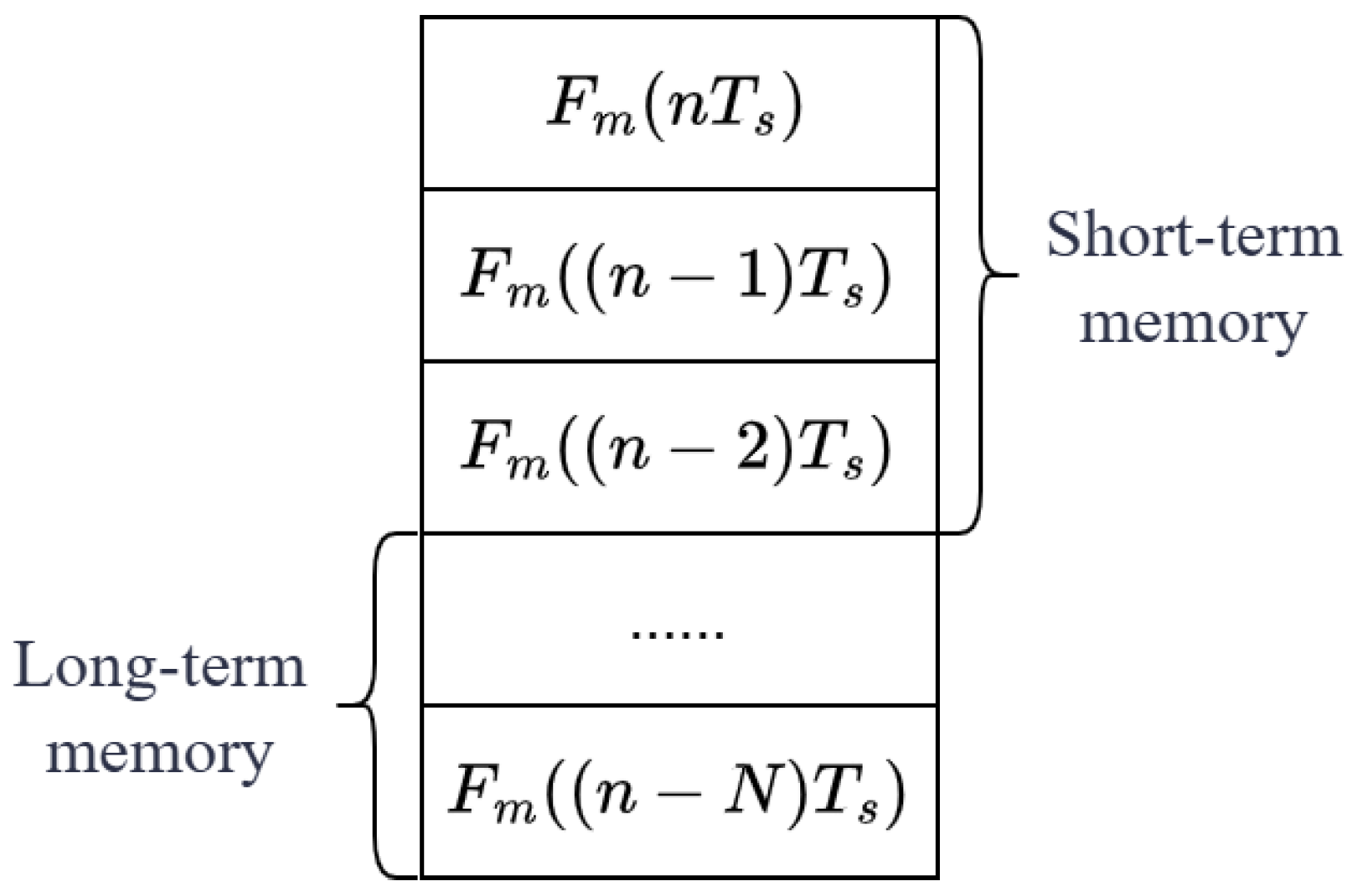
The tensor composed of several adjacent temporal features relative to the current time step is defined as short-term memory, while features from earlier time steps are referred to as long-term memory. Target characteristics in short-term memory typically exhibit minimal variation, whereas those in long-term memory may undergo more significant changes. The schematic illustration of temporal feature classification is presented in Figure 9.
The raw array-domain data of active sonar time-series echoes undergo preprocessing steps including frequency diversity, filtering, and effective echo extraction. Using the feature extraction method described in Section 2.1, the temporal feature data of the target in the spatial, time–frequency, and Doppler domains are extracted, denoted as D3SF(nTs), EPWVD(nTs), and DFSD(nTs), respectively. The single-burst memory representations of these time-series features for the three domains are formulated in Equations (15)–(17).
M S ( n ) = F N e t 1 ( D 3 S F ( n T s ) )
M T F ( n ) = F N e t 2 ( E P W V D ( n T s ) )
M D ( n ) = F N e t 3 ( D F S D ( n T s ) )
The short-term memory is constructed by selecting the two most recent bursts preceding the current burst, while the long-term memory incorporates the fourth and sixth bursts prior to the current burst. This configuration forms the multi-domain temporal echo features of underwater targets, as illustrated in Figure 10.
By integrating the short-term and long-term memory of multi-domain temporal features, the fused representation of target scattering echoes is derived. This approach has the potential to mitigate the instability of echo characteristics induced by underwater acoustic channel fluctuations and variations in target aspect angles, thereby enhancing the accuracy of target recognition.

2.3. Network Construction

2.3.1. Multi-Domain Feature Extractor

HasNet-5, TFasNet-7, and DasNet-9, shown in Figure 1, are specifically designed according to the image characteristics of feature spectra in the spatial, time–frequency, and Doppler domains [18], with their corresponding network architectures detailed in Table 1.
HasNet-5 comprises two components: the feature extractor ϕ H a s N e t - 5 F and the classifier ϕ H a s N e t - 5 C . The spatial domain feature D 3 S F n ( θ , ψ ) R H × W is converted into a tensor, which is denoted as Ts.
T s = T e n s o r ( D 3 S F n ) R H × W
The tensor Ts is processed by ϕ H a s N e t - 5 F , yielding the high-order spatial domain feature vector Fs.
F s = ϕ H a s N e t - 5 F ( T s , Θ s F )
where Θ s F denotes the network parameters of the feature extractor, which can be expressed as
Θ s F = W ( 1 ) , b ( 1 ) , W ( 1 ) , b ( 1 ) , , W ( L ) , b ( L )
where, L represents the length of the network parameters. Then, HasNet-5 can be expressed as
ϕ H a s N e t - 5 ( T s ) = ϕ H a s N e t - 5 C ( ϕ H a s N e t - 5 F ( T s , Θ s F ) , Θ s C ) = ϕ H a s N e t - 5 C ( F s , Θ s C )
where Θ s C denotes the network parameters of the classifier.
The tensors associated with the time–frequency domain feature E P W V D ( t , f ) R H × W and the Doppler domain feature D F S D ( τ , f d ) R H × W are denoted as Ttf and Td, respectively. Consequently, TFasNet-7 and DasNet-9 can be formulated as Equations (22) and (23).
ϕ T F a s N e t - 7 ( T t f ) = ϕ T F a s N e t - 7 C ( ϕ T F a s N e t - 7 F ( T t f , Θ t f F ) , Θ t f C ) = ϕ T F a s N e t - 7 C ( F t f , Θ t f C )
ϕ D a s N e t - 9 ( T d ) = ϕ D a s N e t - 9 C ( ϕ D a s N e t - 9 F ( T d , Θ d F ) , Θ d C ) = ϕ D a s N e t - 9 C ( F d , Θ d C )
The components ϕ T F a s N e t - 7 F and ϕ T F a s N e t - 7 C denote the feature extractor and classifier of TFasNet-7, with network parameters Θ t f F and Θ t f C , respectively. Similarly, ϕ D a s N e t - 9 F and ϕ D a s N e t - 9 C represent the corresponding modules in DasNet-9, parameterized by Θ d F and Θ d C . The resulting high-order feature vectors Ftf and Fd correspond to the time–frequency domain and Doppler domain, respectively. HasNet-5, TFasNet-7, and DasNet-9 were independently trained on the training sets corresponding to the spatial, time–frequency, and Doppler domains, respectively, resulting in three feature extractors— ϕ H a s N e t - 5 F , ϕ T F a s N e t - 7 F , and ϕ D a s N e t - 9 F —with learned parameter sets Θ s F 0 , Θ t f F 0 , and Θ d F 0 .

2.3.2. Internal Memory Module

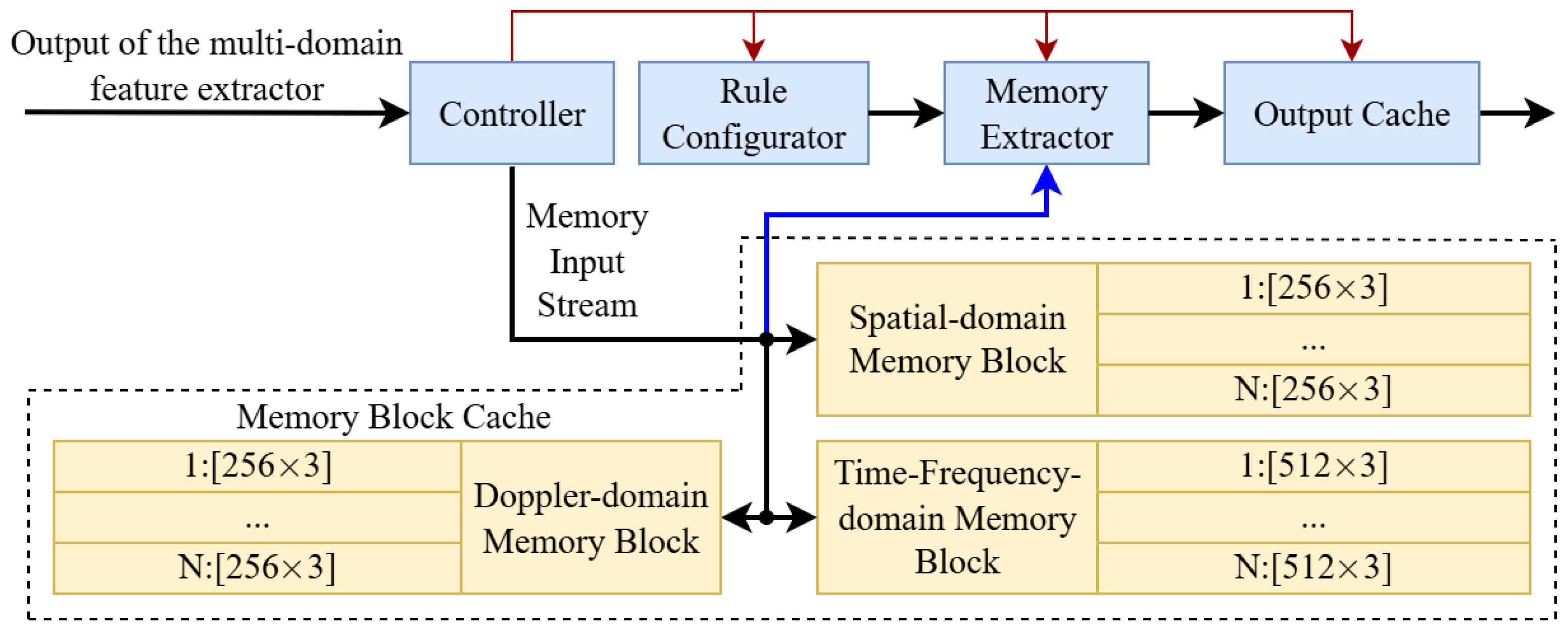
This paper employs a feature vector-level multi-domain temporal feature fusion network in which the feature vectors generated by the multi-domain feature extractor from time-series echoes form the feature memory. The internal memory module manages the stored memory and serves as an intermediary component by providing input to the multi-domain temporal feature fusion classifier, thereby fulfilling a bridging role within the overall architecture [28]. As illustrated in Figure 11, the internal memory module comprises five key components: a controller, a memory block cache, a rule configurator, a memory extractor, and an output cache.
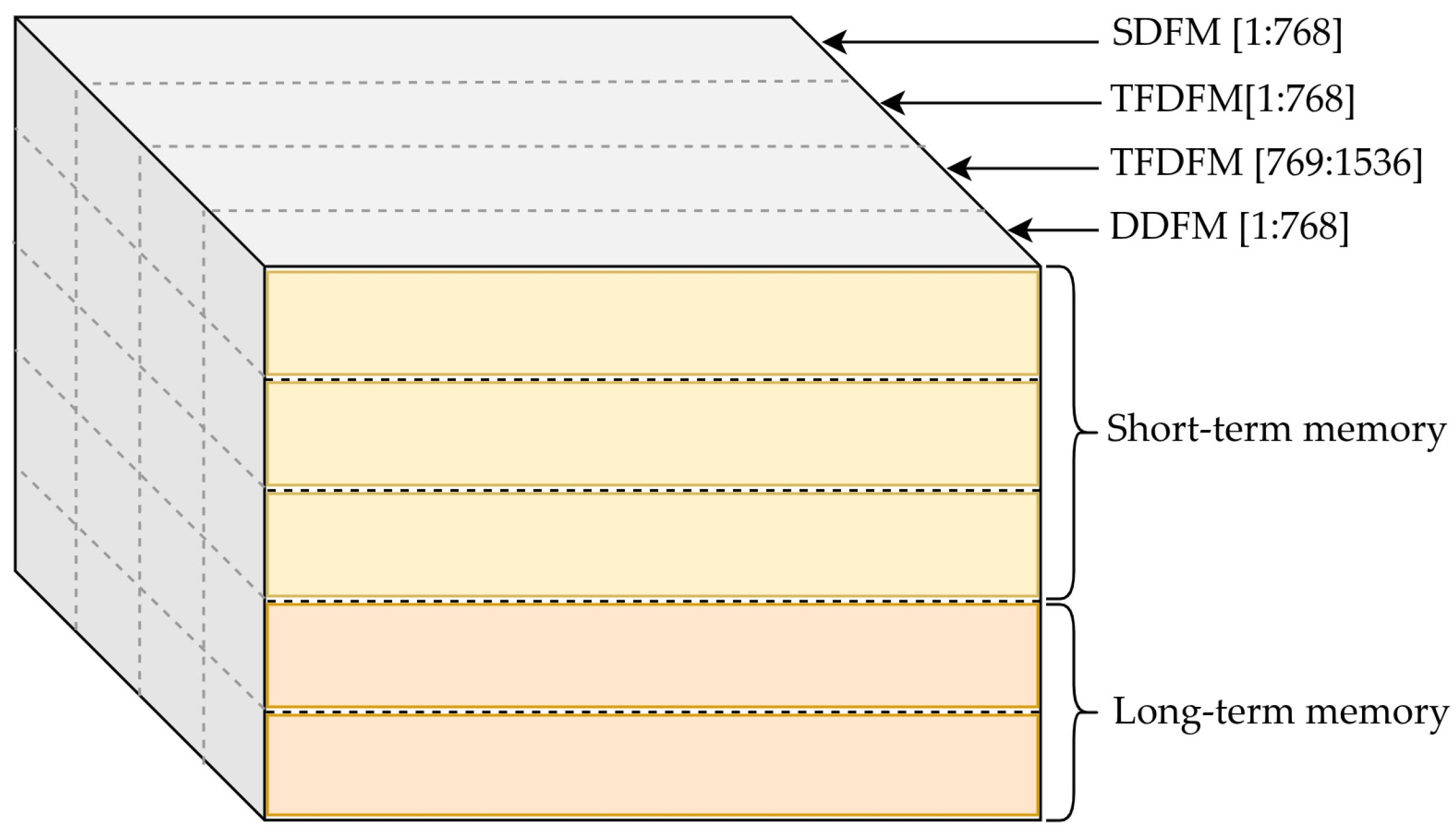
The controller receives the feature vectors output by the multi-domain feature extractor, classifies them into designated categories, and stores them in the memory block cache, while coordinating the operations of other modules. The rule configurator specifies the memory selection policy; for instance, as illustrated in Figure 10, the predefined priority rule is [n, n − 1, n − 2, n − 3, n − 6]. According to this rule, the memory extractor retrieves selected entries from the memory block cache and organizes them into a memory tensor, which is then stored in the output cache. The resulting output memory tensor, derived based on the configuration in Figure 10, is depicted in Figure 12.
In Figure 12, SDFM denotes the spatial domain feature map, TFDFM the time–frequency domain feature map, and DDFM the Doppler domain feature map. The memory tensor contains temporal feature data from three domains—spatial, time–frequency, and Doppler—spanning five bursts. The feature vector length per burst is 768 for the spatial domain, 1562 for the time–frequency domain multi-resolution features, and 768 for the Doppler domain. The time–frequency multi-resolution feature vector is uniformly partitioned into two equal groups. As a result, the high-dimensional temporal features are compressed into an internal memory tensor of size 5 × 4 × 768. By adjusting the rule definition according to specific application needs, different configurations of multi-domain temporal feature vector memories can be generated.

2.3.3. Multi-Domain Temporal Feature Fusion Classifier

The Multi-domain Temporal Feature Fusion Classifier (MT-FFC) integrates feature vectors from multi-domain temporal features and extracts high-dimensional statistical characteristics to enable target classification. The classifier comprises a 3D convolutional layer (Conv3D1) and a fully connected linear layer (Linear1), with its computational procedure defined in Equation (24).
ϕ M T - F F C ( F m s ) = ϕ L i n e a r 1 C ( ϕ C o n v 3 D 1 F ( F m s , Θ C o n v 3 D 1 F ) , Θ L i n e a r 1 C ) = ϕ L i n e a r 1 C ( F m , Θ L i n e a r 1 C )
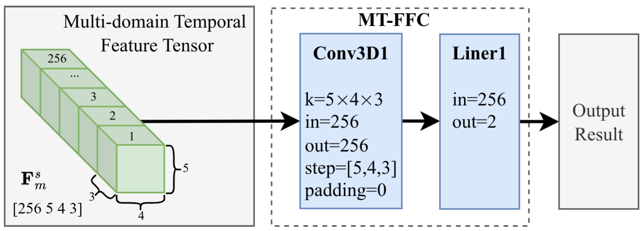
The network architecture of MT-FFC under the memory selection rule [0, 1, 2, 3, 5] is illustrated in Figure 13.
In Figure 13, the input to Conv3D1 is a four-dimensional feature tensor of size [256, 5, 4, 3], and the layer outputs a 256-dimensional vector. The convolutional kernel size is [5, 4, 3], with a stride of [5, 4, 3] and no padding applied. The convolution operation is implemented using Conv3D. The first fully connected linear layer (Linear1) takes the 256-neuron one-dimensional output vector from Conv3D1 as input. The second fully connected layer consists of two neurons, and applies the softmax function to produce the probabilities for the two target classes.

2.3.4. Multi-Domain Temporal Feature Fusion Recognition Network

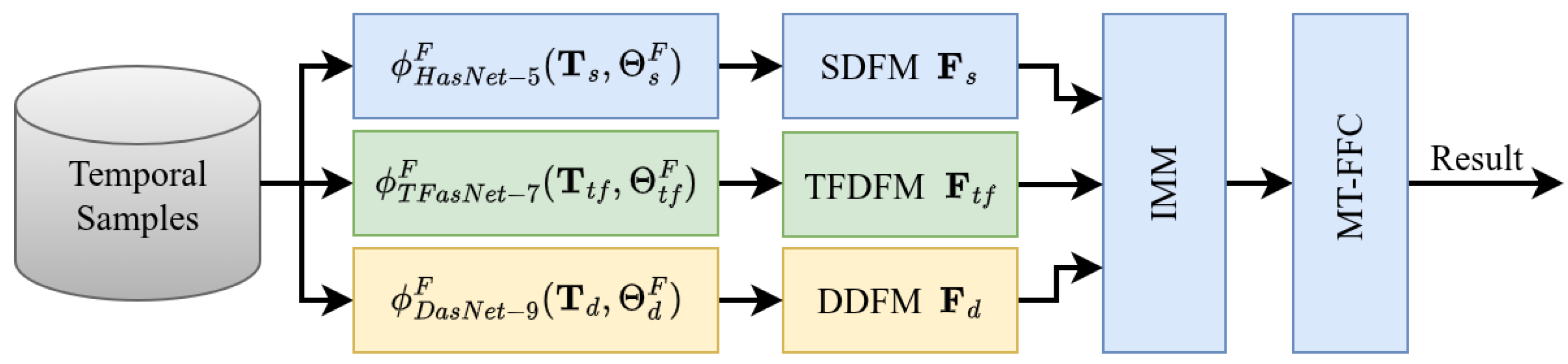
The fusion of multi-burst feature information across the spatial, time–frequency, and Doppler domains enables statistical characterization of target features in both the feature and temporal dimensions, thereby mitigating information bias and effectively addressing the instability of target scattering characteristics. The internal memory module stores the multi-burst feature vector outputs from the multi-domain feature extractor, which are subsequently classified by MT-FFC. This integration leads to the construction of the Multi-domain Temporal Feature Fusion Recognition Network (MTFF-RNet), whose overall architecture is illustrated in Figure 14.
In Figure 14, time-series samples from the training library are sequentially fed into the multi-domain feature extractor in chronological order. The extracted feature vectors from the spatial, time–frequency, and Doppler domains are transmitted to the internal memory module, which generates a multi-domain temporal feature tensor (256 × 5 × 4 × 3) at each time step. These tensors serve as input to the MT-FFC for target classification. The parameters of the multi-domain feature extractor are kept fixed during training, while the MT-FFC is fully trained on the accumulated feature sequences, resulting in a well-structured inference network for multi-domain temporal feature fusion target recognition.

3. Results and Discussion

3.1. Dataset

The dataset employed in this study comprises three components: a training set, a validation set, and a test set. Underwater vehicles (volume target) are designated as true targets, while multi-source interferences are treated as false targets. From the experimental data, effective continuous multi-burst sequences are selected, including 22 groups of interference time series samples and 10 groups of underwater vehicle time series samples. Of these, 8 groups are allocated to the training set, 10 to the validation set, and the remaining 15 to the test set, with each group containing 12 to 20 individual samples. To ensure independence and avoid data leakage, the training set is constructed using data from different experimental runs than those used for the validation and test sets.
Due to the limited availability of experimental data, simulated echo signals are generated based on acoustic principles to augment the dataset. The simulation process employs highlight models of typical underwater vehicles and four types of multi-source interferences [18,29] to synthesize sonar array-domain data. The active sonar system consists of a 25-element array configured as [1, 3, 5, 5, 3, 1], transmitting both CW and LFM waveforms with a pulse duration of 65 ms. Simulations are conducted under a representative tail-following target scenario. Initial conditions for signal generation include an azimuth angle θ ranging from 15° to 90° (in 5° increments, yielding 16 values), a pitch angle of −1°, an initial target range of 525 m, target speeds between 15 and 25 knots, sonar platform speeds from 25 to 30 knots, and lead angles varying from 2° to 8°. Data generation terminates when the target range decreases below 210 m. The SNR ranges from −9 dB to 9 dB. Reverberation is either absent, or the signal-to-reverberation ratio (SRR) ranges from −3 dB to 3 dB. This process yields 160 groups of time series data across five target classes. From these, 40 groups are assigned to the training set, 18 to the validation set, and 17 to the test set, with each group consisting of 12 to 20 samples. During the data generation process, it is essential to ensure that parameters such as the trajectories and initial azimuth angles of the validation and test data differ from those of the training data. Additionally, adjustments should be made to parameters including the number of highlights, their intensity, and the speed of the target model.
The final multi-domain feature datasets—MFTD (training), MFVD (validation), and MFRD (test)—are formed by combining the above 107 time series sample groups, comprising 32 experimentally acquired and 75 simulated samples. The detailed composition of the multi-domain feature sample sets is summarized in Table 2.
From the 107 groups of time series samples, multi-domain temporal feature samples are extracted to construct the training set MFTsTD, validation set MFTsVD, and test set MFTsRD. The extraction protocol begins at the sixth cycle of a given voyage sequence, from which five consecutive cycles of multi-domain features are collected to form a single training instance. The selected cycles include the first, second, third, fifth, and sixth cycles. Each time series multi-domain feature sample is represented as a four-dimensional tensor, denoted by T m s , as defined in Equation (25).
T m s = { T m n , T m n 1 , T m n 2 , T m n 3 , T m n 5 }
where T m n is a three-dimensional tensor formed by feature vectors from the spatial, time–frequency, and Doppler domains, as defined in Equation (26).
T m n = { T s n , T t f n , T d n }
Then, sequential extraction proceeds from the seventh cycle to the final cycle Nlast of the voyage, yielding a total of (NLast − 5) samples for this voyage. The sample composition of the multi-domain temporal feature set is presented in Table 3.

3.2. Evaluation Metrics

During the network training process, classification accuracy is used as the evaluation metric, as defined in Equation (27) [30].
A c c u r a c y = T P + T N T P + T N + F P + F N
Here, TP denotes true positive cases, TN denotes true negative cases, FP represents false positive cases, and FN represents false negative cases. During the inference stage, the network performance is evaluated using precision, recall, and the F1-score, as defined in Equations (28)–(30) [30]. Furthermore, to provide a threshold-invariant and class-imbalance-robust evaluation—particularly critical for skewed datasets—we compute the area under the precision–recall curve (AUC-PR) and its 95% confidence interval (CI), estimated using bootstrap resampling with 1000 independent replicates [31].
p r e c i s i o n = T P T P + F P
r e c a l l = T P T P + F N
F 1 = 2 × P r e c i s i o n × R e c a l l P r e c i s i o n + R e c a l l

3.3. Validation

3.3.1. Overview of the Validation Process

First, based on the multi-domain feature extraction network constructed in Section 2.3.1, spatial, time–frequency, and Doppler domain feature extractors are independently trained on the training set MFTD described in Section 3.1 and validated using the validation set MFVD. Second, on the training set MFTsTD, the multi-domain temporal feature fusion classifier MT-FFC—developed in Section 2.3.3—is trained within the MTFF-RNet framework introduced in Section 2.3.4 and validated on MFTsVD. Subsequently, the trained feature extractors and MT-FFC are integrated to form the MTFF-RNet inference network, which is evaluated and analyzed on the temporal test set MFTsRD. Finally, the proposed multi-domain temporal fusion-based target recognition method is further assessed through comparative experiments with the multi-domain feature fusion network and four lightweight models.

3.3.2. Multi-Domain Feature Extractor Training

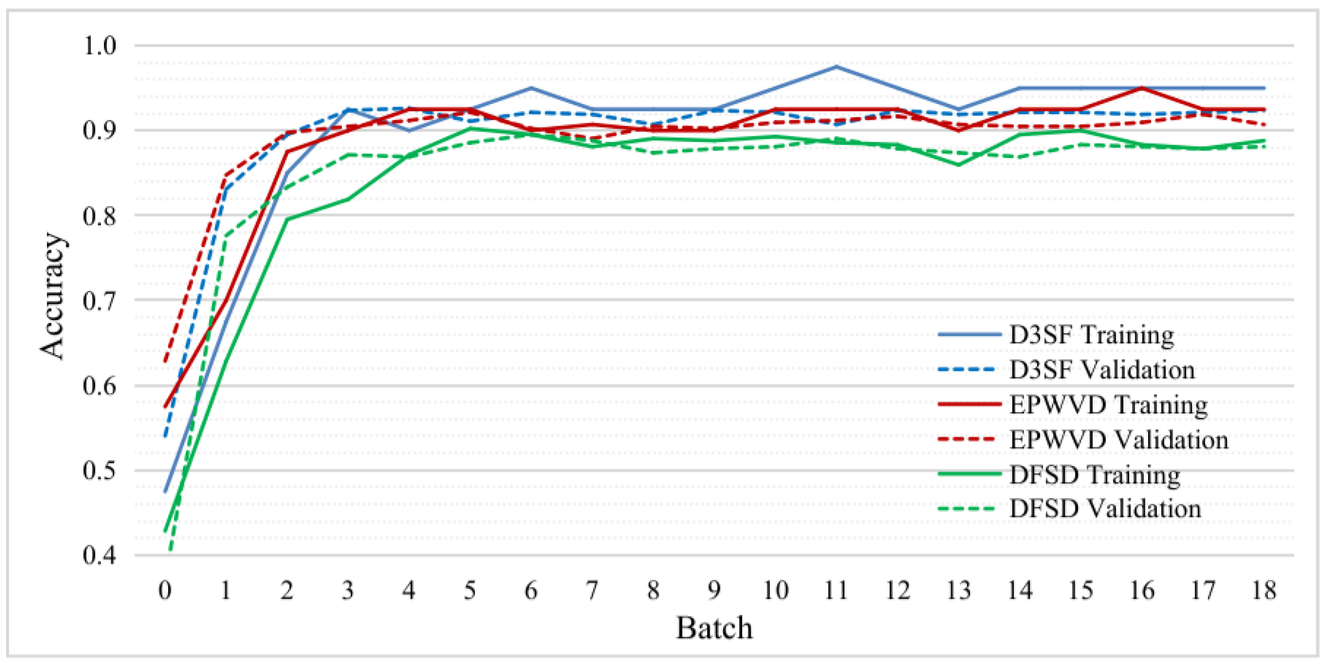
The meta-knowledge (MK_S, MK_TF, and MK_D) [18] obtained from the pre-training of meta-learning is used to initialize the network parameters of the feature extractors of HasNet-5, TFasNet-7, and DasNet-9, in order to reduce the sample requirement and improve the training efficiency. The three networks are independently trained using the spatial domain, time–frequency domain, and Doppler domain samples of the training set MFTD (with a learning rate of 0.005), and the validation set MFVD samples are used for evaluation during the training process. The training curves and validation curves are shown in Figure 15.
In Figure 15, each training batch on the horizontal axis corresponds to 40 samples. As shown in the validation curves, after two training batches using meta-knowledge, the validation accuracy of the individual feature recognition networks for spatial, time–frequency, and Doppler domains reaches 89.52%, 89.76%, and 83.3%, respectively. Upon completion of one full training epoch, the models achieve convergence, with the validation accuracy stabilizing at 92.38%, 90.71%, and 88.10%, respectively. After training, inference testing is performed on the test set, yielding test accuracy rates of 91.87%, 90.42%, and 87.50% for the spatial, time–frequency, and Doppler features, respectively. The D3SF feature in the spatial domain exhibits minimal variation in classification accuracy across different azimuth angles. In contrast, the EPWVD feature in the time–frequency domain suffers from degraded performance near an azimuth angle of 90° due to insufficient time–frequency resolution. Similarly, the DFSD feature in the Doppler domain shows reduced classification accuracy when the azimuth angle is below 30°.

3.3.3. MT-FFC Training

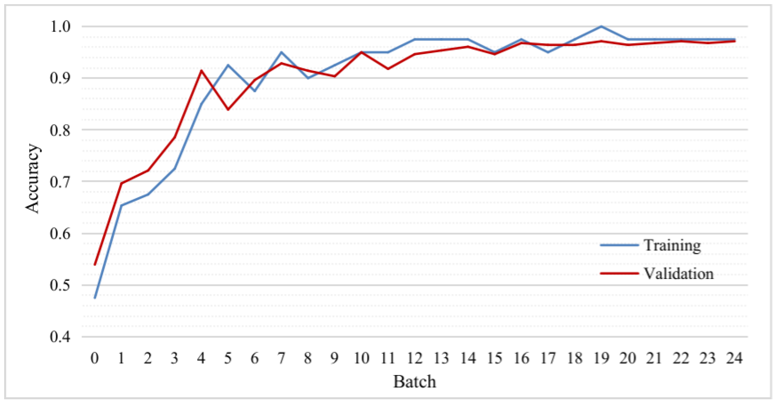
Network training was conducted on the time-series feature training set MFTsTD using a learning rate of 0.001. During training, only the parameters of MT-FFC were updated, while the parameters of the multi-domain feature extractor were fixed to preserve pre-trained domain-specific features. The validation set was employed to assess the training performance. The resulting training and validation curves are presented in Figure 16.
After seven training batches (each batch comprising 40 samples), the validation accuracy surpassed 90%, and the MT-FFC network began to converge. The entire training process encompassed two complete training epochs, with each epoch consisting of 12 batches. As evidenced by the validation curve, the fusion of multi-domain temporal features enabled the model to achieve the desired target classification performance, ultimately attaining a classification accuracy of 97.14% upon completion of the two training epochs.

3.3.4. MTFF-RNet Testing

Following the completion of MT-FFC training, the inference-capable MTFF-RNet network was developed based on the architecture illustrated in Figure 14. The model was evaluated on the test set MFTsRD to assess its inference performance, and the results are summarized in Table 4.
As shown in Table 4, the simulation samples achieved an accuracy of 96.47%, with a precision of 87.5%, recall of 93.33%, and F1-score of 90.32%. These samples consisted of 30 true target instances and 140 false target instances. Four false targets were misclassified as true targets; further analysis revealed that two of these cases exhibited interface reverberation. For the experimental samples, the model achieved an accuracy of 96.00%, precision of 93.55%, recall of 96.67%, and F1-score of 95.08%. The experimental samples included 60 true target samples and 90 false target samples. Among the classification errors, two true targets were incorrectly classified as false (due to large distance and interface reverberation), and four false targets were misclassified as true. Notably, two of the erroneous classifications involved samples with interface reverberation. Across all test samples, including both simulation and experimental datasets, the overall performance achieved an accuracy of 96.25%, a precision of 91.49%, a recall of 95.56%, and an F1-score of 93.48%. The consistent improvement across all four evaluation metrics indicates that the fusion of multi-domain temporal features effectively mitigates the adverse impact of unstable echo signals on recognition performance.

3.4. Discussion

3.4.1. Ablation Studies

In Section 3.3, the temporal feature extraction employs memory rule MR4: [n, n − 1, n − 2, n − 3, n − 5]. To systematically assess the influence of temporal context length on recognition performance, this section introduces three ablated variants—MR3: [n, n − 1, n − 2, n − 3], MR2: [n, n − 1, n − 2] and MR1: [n, n − 1]. For each rule, the depth dimension of MT-FFC’s 3D convolutional kernel is explicitly adapted to match the number of input frames, ensuring architectural consistency. All models are trained and evaluated under identical experimental protocols. Comparative inference results across MR1, MR2, MR3, and MR4 are summarized in Table 5.
The ablation study on memory rules reveals a clear trade-off: increasing the temporal context length enhances the robustness of target recognition at the cost of higher computational complexity and increased inference latency. Consequently, the optimal memory rule must be selected based on application-specific constraints—such as real-time processing requirements, hardware resource limitations, and operational tolerance for performance degradation.

3.4.2. Stratified Evaluation Metrics

Given the pronounced degradation in spatial resolution of the D3SF feature spectrum below an SNR of 3 dB—contrasting with the comparatively stable resolution performance of both EPWVD and DFSD feature spectra—the test samples are stratified into two groups: one comprising all samples with SNR ≥ 3 dB and the other comprising those with SNR < 3 dB. Separate evaluations are performed on each group, and the corresponding results are summarized in Table 6.
As shown in Table 6, the target recognition performance of MTFF-RNet degrades with decreasing SNR, confirming that misclassifications predominantly occur among low-SNR samples. This degradation is primarily attributable to the pronounced deterioration of D3SF feature discriminability under low-SNR conditions—particularly for targets located at longer ranges and with azimuth angles near 90°, where resolution limitations impede reliable separation. Nevertheless, the model achieves strong overall performance, as evidenced by an accuracy of 95.71%, precision of 88.57%, recall of 93.94%, F1-score of 91.18%, and AUC-PR of 93.88%, all of which collectively indicate robust and practically viable recognition capability.
Given the pronounced resolution degradation observed in both the D3SF and EPWVD feature spectra below a SRR of 3 dB—contrasting with the comparatively stable resolution behavior of the DFSD feature spectrum—the test samples are stratified into two groups: one comprising all samples with SRR ≥ 3 dB, and the other comprising those with SRR < 3 dB. Separate evaluations are conducted on each group, and the corresponding results are summarized in Table 7.
As shown in Table 7, MTFF-RNet exhibits a pronounced decline in target recognition performance under low SRR conditions—confirming that SRR is a critical factor governing recognition robustness in underwater environments, a challenge widely acknowledged in the literature. This observed degradation primarily stems from the diminished discriminability of weak highlight features used to distinguish volume targets from multi-source interference. Addressing this limitation constitutes a key focus of our ongoing work. Nevertheless, the model achieves consistently strong performance across multiple metrics: accuracy of 94.44%, precision of 84.00%, recall of 91.30%, F1-score of 87.50%, and AUC-PR of 91.04%—collectively demonstrating operationally viable recognition capability even under challenging SRR conditions.

3.4.3. Performance Comparison

To further evaluate the target classification capability of MTFF-RNet, comparative experiments were conducted against five lightweight networks: ResNet18, MobileNetV2, ShuffleNetV2x1, EfficientNetB0, and MFasNetV1 [15,18,32,33,34,35]. Among these, ResNet18 and the other three lightweight architectures employ feature level fusion for classification, whereas MFasNetV1 adopts multi-domain feature fusion at the feature vector level. All five models were trained on the MFTD training set under consistent conditions. During inference comparison, a key distinction arises: MTFF-RNet processes multi-domain time-series feature samples, while the competing networks operate on multi-domain single-burst feature inputs. To ensure a fair evaluation, the test set for the baseline networks was constructed by excluding the first five sequential samples from both the experimental and simulation voyage sequences used in MTFF-RNet’s temporal modeling, resulting in a final test set comprising 150 experimental and 170 simulated samples. The complete inference results on the MFTsRD test set are summarized in Table 8.
As shown in Table 5, MTFF-RNet consistently outperforms ResNet18, MobileNetV2, EfficientNetB0, and ShuffleNetV2x1 across all evaluation metrics. MTFF-RNet shares an identical feature extractor and pre-training reference with MFasNetV1; the key distinction lies in the fusion strategy—MFasNetV1 integrates multi-domain features from a single time step, whereas MTFF-RNet incorporates multi-domain temporal features over sequential time steps. Compared to MFasNetV1, MTFF-RNet achieves improvements of 3.12% in accuracy, 6.07% in precision, 4.45% in recall, 5.31% in F1-score, and 0.84% in AUC-PR. The comparative experimental results demonstrate that the multi-domain temporal feature fusion network TMFF-RNet, based on feature vector-level fusion, significantly enhances the recognition accuracy under water acoustic channel fluctuations and dynamic variations in target perspectives, thereby achieving superior performance in addressing the target recognition problem in this study. Although the total number of parameters and FLOPs in MTFF-RNet are lower than those in ResNet-18, its overall parameter count exceeds that of lightweight networks such as MobileNetV2, ShuffleNetV2x1, and EfficientNet-B0. However, the three feature extractors in MTFF-RNet are trained independently, with each subnetwork having a parameter scale comparable to that of MobileNetV2 or ShuffleNetV2x1. Furthermore, parameter initialization leverages meta-knowledge acquired through meta-learning [17], granting MTFF-RNet a distinct advantage in few-shot scenarios.
Compared to MobileNetV2 and EfficientNetB0, TMFF-RNet does not exhibit significant advantages in parameter count or overall computational complexity. Nevertheless, its multi-stream feature extraction architecture combined with a modular training strategy offers distinct benefits in scenarios characterized by limited and imbalanced data. Furthermore, the structural design of the multi-domain feature extractor facilitates distributed deployment across multiple AI accelerators, enabling enhanced real-time processing capabilities. The proposed feature-vector-level fusion approach for multi-domain temporal feature recognition effectively integrates target information across both domain-specific features and temporal dynamics, thereby improving the adaptability of recognition models under low-data conditions. This framework presents a novel perspective on information fusion for identifying targets with dynamically evolving characteristics in complex and non-stationary environments—such as those subject to environmental fluctuations and interference-induced data instability. Additionally, the internal memory mechanism supports flexible rule configurations, allowing adaptation to scenarios with varying rates of change. Different configuration strategies yield diverse high-dimensional statistical representations, which can serve as valuable references for future designs of multi-stream temporal fusion systems.

4. Conclusions

This paper addresses the challenge of performance instability in active sonar target recognition under limited sample conditions, caused by fluctuations in underwater acoustic channels and variations in target aspect angles. To overcome the limitations of conventional methods relying on a single feature or single-ping echoes, we propose a multi-domain temporal feature fusion approach. First, complementary features—namely D3SF, EPWVD, and DFSD—were extracted from the spatial, time–frequency, and Doppler domains, respectively. Second, a deep learning framework was developed for the feature vector-level fusion of multi-domain temporal echo characteristics. Building on this foundation, an efficient internal memory module and a multi-domain temporal feature fusion classifier were designed, resulting in the proposed MTFF-RNet, which is capable of capturing high-dimensional statistical patterns. The network was trained and evaluated using a hybrid dataset combining real experimental measurements with simulation-augmented samples. The experimental results showed an inference accuracy of 96.25% and an F1-score of 93.48%. To assess the contribution of memory utilization and evaluate the model’s robustness across diverse acoustic environments, we conducted ablation studies, SNR-stratified experiments, and SRR-stratified experiments. Performance comparisons with MFasNetV1 and four feature-level fusion networks demonstrated that the proposed multi-domain temporal fusion method effectively mitigates the performance degradation caused by channel instability and aspect-angle variability. By jointly leveraging multi-domain representations and temporal dynamics, the proposed method integrates target information more comprehensively, offering a novel solution to improve the environmental adaptability of recognition algorithms in data-scarce scenarios. Moreover, the fusion rules for multi-domain temporal integration are highly flexible, allowing different configurations to yield distinct performance trade-offs. Based on this framework, future work will explore two key directions: (i) adaptive memory regulation mechanisms and (ii) systematic multi-dimensional feature fusion for improved cross-domain temporal modeling.

Author Contributions

Conceptualization, X.L. and Y.Y.; methodology, X.L.; software, C.W. and X.L.; validation, X.L., Y.Y., Y.H., X.Y. and J.L.; formal analysis, C.W. and Y.H.; investigation, X.L., X.Y. and Y.H.; resources, X.Y. and C.W.; data curation, C.W. and X.Y.; writing—original draft preparation, X.L.; writing—review and editing, X.L., Y.Y., Y.H. and J.L.; visualization, X.L. and C.W.; Supervision, Y.Y. All authors have read and agreed to the published version of the manuscript.

Funding

This research received no external funding.

Institutional Review Board Statement

Not applicable.

Informed Consent Statement

Not applicable.

Data Availability Statement

Data are contained within the article.

Acknowledgments

The authors appreciate the linguistic assistance from Xiaojia Jiao during the revision of this paper.

Conflicts of Interest

The authors declare no conflicts of interest.

Abbreviations

The following abbreviations are used in this manuscript:
ASTRActive Sonar Target Recognition
CNNConvolutional Neural Network
CWTContinuous Wavelet Transform
D3SFThree-dimensional Spatial Feature
DFSDDoppler Frequency Shift Distribution
FFCFeature Fusion Classifier
IMMInternal Memory Module
MFCCMel-Frequency Cepstral Coefficients
MSIMulti-Source Interference
MUSICMultiple Signal Classification
PWVDPseudo Wigner–Ville Distribution
SPWVDSmoothed Pseudo Wigner–Ville Distribution
WVDWigner–Ville Distribution Spectrum

References

  1. Aubard, M.; Madureira, A.; Teixeira, L.; Pinto, J. Sonar-Based Deep Learning in Underwater Robotics: Overview, Robustness, and Challenges. IEEE J. Ocean. Eng. 2025, 50, 1866–1884. [Google Scholar] [CrossRef]
  2. Feng, S.; Ma, S.; Zhu, X.; Yan, M. Artificial Intelligence-Based Underwater Acoustic Target Recognition: A Survey. Remote Sens. 2024, 16, 3333. [Google Scholar] [CrossRef]
  3. Yang, H.; Byun, S.H.; Lee, K.; Choo, Y.; Kim, K. Underwater acoustic research trends with machine learning: Active SONAR applications. J. Ocean Eng. Technol. 2020, 34, 277–284. [Google Scholar] [CrossRef]
  4. Luo, X.; Chen, L.; Zhou, H.; Cao, H. A Survey of Underwater Acoustic Target Recognition Methods Based on Machine Learning. J. Mar. Sci. Eng. 2023, 11, 384. [Google Scholar] [CrossRef]
  5. Darmon, M.; Dorval, V.; Baqué, F. Acoustic Scattering Models from Rough Surfaces: A Brief Review and Recent Advances. Appl. Sci. 2020, 10, 8305. [Google Scholar] [CrossRef]
  6. Abraham, D.A. Underwater Acoustics Signal Processing Modeling, Detection, and Estimation; Springer: Cham, Switzerland, 2019; pp. 95–196. [Google Scholar] [CrossRef]
  7. Zhao, S.; Li, L.; Zhang, X.; Zhang, D.; Li, M. Simulation of backscatter signal of submarine target based on spatial distribution characteristics of target intensity. In Proceedings of the 2021 OES China Ocean Acoustics, Harbin, China, 14–17 July 2021; pp. 234–239. [Google Scholar] [CrossRef]
  8. Chen, Y.; Guo, Y. Optimal Combination Strategy for Two Swim-Out Acoustic Decoys to Countermeasure Acoustic Homing Torpedo. In Proceedings of the 2017 4th International Conference on Information Science and Control Engineering (ICISCE), Changsha, China, 21–23 July 2017; pp. 1061–1065. [Google Scholar] [CrossRef]
  9. Wang, Z.; Wu, J.; Wang, H.; Hao, Y.; Wang, H. A Torpedo Target Recognition Method Based on the Correlation between Echo Broadening and Apparent Angle. Appl. Sci. 2022, 12, 12345. [Google Scholar] [CrossRef]
  10. Malarkodi, A.; Manamalli, D.; Kavitha, G.; Latha, G. Acoustic Scattering of Underwater Targets. In Proceedings of the 2013 Ocean Electronics (SYMPOL), Kochi, India, 23–25 October 2013; pp. 127–132. [Google Scholar] [CrossRef]
  11. Stinco, P.; Tesei, A.; LePage, K.D. Unsupervised Active Sonar Contact Classification through Anomaly Detection. EURASIP J. Adv. Signal Process. 2023, 2023, 59. [Google Scholar] [CrossRef]
  12. Wang, Q.; Du, S.; Wang, F.; Chen, Y. Underwater target recognition method based on multi-domain active sonar echo images. In Proceedings of the 2021 IEEE International Conference on Signal Processing, Communications and Computing (ICSPCC), Xi’an, China, 17–19 August 2021; pp. 1–5. [Google Scholar] [CrossRef]
  13. Wang, Q.; DU, S.; Zhang, W.; Wang, F. Active sonar target recognition method based on multi-domain transformations and attention-based fusion network. IET Radar Sonar Navig. 2024, 18, 1814–1828. [Google Scholar] [CrossRef]
  14. Chen, Y.; Liang, H.; Dai, Z. Differentiable Architecture Search with Multi-Domain Time-Frequency Features for Underwater Target Recognition. In Proceedings of the OCEANS 2025 Brest, Brest, France, 16–19 June 2025; pp. 1–4. [Google Scholar] [CrossRef]
  15. Chen, Y.; Liang, H.; Li, H.; Song, S. A Lightweight Time–Frequency–Space Dual-Stream Network for Active Sonar-Based Underwater Target Recognition. IEEE Sens. J. 2025, 25, 11416–11427. [Google Scholar] [CrossRef]
  16. Dai, Z.; Liang, H.; Duan, T.; Yue, L.; Gou, W.; Zhu, W. Active Sonar Target Recognition Based on Sub-Beam Filling and Time-Frequency Fusion Tensor. Appl. Acoust. 2025, 239, 110864. [Google Scholar] [CrossRef]
  17. Chen, Y.; Liang, H.; Li, H.; Gou, W.; Zhu, L. PBGMR: A Physics-Informed Bayesian Graph Neural Network for Robust Multimodal Underwater Target Recognition. IEEE Trans. Instrum. Meas. 2025, 74, 6508312. [Google Scholar] [CrossRef]
  18. Liu, X.; Yang, Y.; Hu, Y.; Yang, X.; Liu, L.; Shi, L.; Liu, J. A Meta-Learning-Based Recognition Method for Multidimensional Feature Extraction and Fusion of Underwater Targets. Appl. Sci. 2025, 15, 5744. [Google Scholar] [CrossRef]
  19. Dai, Z.; Liang, H.; Chen, Y. An underwater moving target recognition method based on inter-frame motion feature cyclic reconstruction. In Proceedings of the OCEANS 2024—Halifax, Halifax, NS, Canada, 23–26 September 2024; pp. 1–5. [Google Scholar] [CrossRef]
  20. Xiang, W.; Song, Z.; Gao, Z.; Zhang, B.; Fu, W.; Zhang, C.; Zhang, Y. Underwater target classification based on the combination of dolphin click trains and convolutional neural networks. J. Acoust. Soc. Am. 2025, 157, 647–658. [Google Scholar] [CrossRef] [PubMed]
  21. Zaharis, Z.D.; Gravas, I.P.; Lazaridis, P.I.; Yioultsis, T.V.; Antonopoulos, C.S.; Xenos, T.D. An Effective Modification of Conventional Beamforming Methods Suitable for Realistic Linear Antenna Arrays. IEEE Trans. Antennas Propag. 2020, 68, 5269–5279. [Google Scholar] [CrossRef]
  22. Liu, X.; Yang, Y.; Hu, Y.; Wang, C.; Li, Y. Research on the Extraction and Recognition of Space-Time-Frequency Features for Underwater Moving Targets. J. Unmanned Undersea Syst. 2025, 34, 85–93. [Google Scholar] [CrossRef]
  23. Mulinde, R.; Attygalle, M.; Aziz, S.M. Pre-Processing-Based Performance Enhancement of DOA Estimation for Wideband LFM Signals. In Proceedings of the 2023 IEEE International Radar Conference (RADAR), Sydney, Australia, 6–10 November 2023; pp. 1–6. [Google Scholar] [CrossRef]
  24. Liu, Y.; Wu, P.; Black, A.W.; Anumanchipalli, G.K. A Fast and Accurate Pitch Estimation Algorithm Based on the Pseudo Wigner-Ville Distribution. In Proceedings of the ICASSP 2023—2023 IEEE International Conference on Acoustics, Speech and Signal Processing (ICASSP), Rhodes Island, Greece, 4–10 June 2023; pp. 1–5. [Google Scholar] [CrossRef]
  25. Zou, Y.; Li, X.; Yu, G. Adaptive WVD Cross-Term Removal Method Based on Multidimensional Property Differences. J. Mar. Sci. Appl. 2024, 24, 774–788. [Google Scholar] [CrossRef]
  26. Hague, D.A.; Buck, J.R. The Generalized Sinusoidal Frequency-Modulated Waveform for Active Sonar. IEEE J. Ocean. Eng. 2017, 42, 109–123. [Google Scholar] [CrossRef]
  27. Jiang, W.; Liu, Y.; Wei, Q.; Wang, W.; Ren, Y.; Wang, C. A High-Resolution Radar Automatic Target Recognition Method for Small UAVs Based on Multi-Feature Fusion. In Proceedings of the 2022 IEEE 25th International Conference on Computer Supported Cooperative Work in Design (CSCWD), Hangzhou, China, 4–6 May 2022; pp. 775–779. [Google Scholar] [CrossRef]
  28. Graves, A.; Wayne, G.; Reynolds, M.; Harley, T.; Danihelka, I.; Grabska-Barwińska, A.; Colmenarejo, S.G.; Grefenstette, E.; Ramalho, T.; Agapiou, J.; et al. Hybrid Computing Using a Neural Network with Dynamic External Memory. Nature 2016, 538, 471–476. [Google Scholar] [CrossRef]
  29. Liu, X.; Yang, Y.; Hu, Y.; Yang, X.; Li, Y.; Xiao, L. Data Augmentation Based on Highlight Image Models of Underwater Maneuvering Target. Xibei Gongye Daxue Xuebao/J. Northwestern Polytech. Univ. 2024, 42, 417–425. [Google Scholar] [CrossRef]
  30. Dong, W.; Fu, J.; Zou, N.; Zhao, C.; Miao, Y.; Shen, Z. CAF-ViT: A Cross-Attention Based Transformer Network for Underwater Acoustic Target Recognition. Ocean. Eng. 2025, 318, 120049. [Google Scholar] [CrossRef]
  31. Saito, T.; Rehmsmeier, M. The Precision-Recall Plot Is More Informative than the ROC Plot When Evaluating Binary Classifiers on Imbalanced Datasets. PLoS ONE 2015, 10, e0118432. [Google Scholar] [CrossRef]
  32. Veit, A.; Wilber, M.; Belongie, S. Residual networks behave like ensembles of relatively shallow networks. In Advances in Neural Information Processing Systems 29 (NIPS 2016); Curran Associates: San Jose, CA, USA, 2016; pp. 550–558. [Google Scholar]
  33. Sandler, M.; Howard, A.; Zhu, M.; Zhmoginov, A.; Chen, L. MobileNetV2: Inverted residuals and linear bottlenecks. In Proceedings of the IEEE Conference on Computer Vision and Pattern Recognition (CVPR), Salt Lake City, UT, USA, 18–23 June 2018; pp. 4510–4520. [Google Scholar] [CrossRef]
  34. Ma, N.; Zhang, X.; Zheng, H.; Sun, J. ShuffleNet V2: Practical guidelines for efficient CNN architecture design. In Proceedings of the European Conference on Computer Vision (ECCV); Springer: Cham, Switzerland, 2018; pp. 122–138. [Google Scholar] [CrossRef]
  35. Tan, M.; Le, Q. EfficientNet: Rethinking model scaling for convolutional neural networks. In Proceedings of the 36th International Conference on Machine Learning (ICML), Long Beach, CA, USA, 9–15 June 2019; pp. 6105–6114. Available online: https://proceedings.mlr.press/v97/tan19a.html (accessed on 25 November 2025).
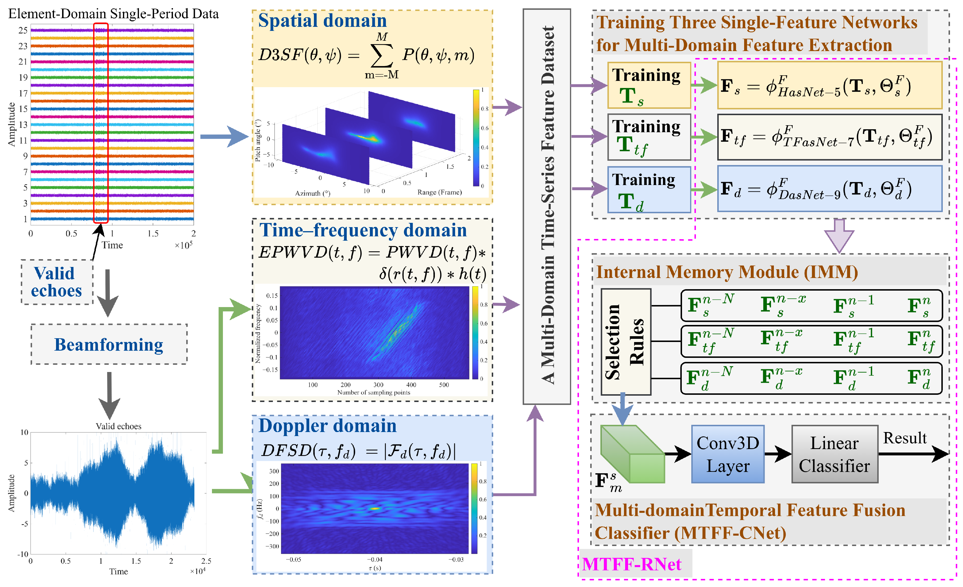
Figure 1. Schematic diagram of target recognition via multi-domain temporal features.
Acoustics 08 00022 g001
Figure 2. D3SF spatial spectrum of MSI and volume targets. The x- and y-axes are labeled in degrees, and the z-axis denotes frame index. (ac) illustrate the D3SF spectra of MSI at an SNR of 12 dB for azimuth angles of 5°, 45°, and 85°, respectively. (df) present the corresponding MSI results at a reduced SNR of 3 dB under identical azimuth configurations. Similarly, (gi) display the D3SF spectra of volume targets at 12 dB SNR with the same set of azimuth angles, while (jl) show the analogous results for volume targets at 3 dB SNR.
Acoustics 08 00022 g002
Figure 3. EPWVD spectra of MSI and volume targets. The x-axis denotes the number of sampling points, and the y-axis denotes the normalized frequency. (ac) illustrate the EPWVD spectra of MSI at an SNR of 0 dB for azimuth angles of 5°, 40°, and 75°, respectively. (df) present the corresponding MSI results under degraded conditions at an SNR of −9 dB with the same azimuth configurations. Similarly, (gi) display the EPWVD spectra of volume targets at 0 dB SNR, while (jl) show the analogous results for volume targets at −9 dB SNR, both spanning the same set of azimuth angles (5°, 40°, and 75°).
Acoustics 08 00022 g003
Figure 4. DFSD spectra of MSI and volume targets. The x-axis is in seconds, and the y-axis is in Hertz. (ac) illustrate the DFSD spectra of MSI at an SNR of 6 dB for azimuth angles of 15°, 50°, and 85°, respectively. (df) present the corresponding MSI results at a lower SNR of 0 dB under the same azimuth configurations. Similarly, (gi) display the DFSD spectra of volume targets at 6 dB SNR with identical azimuth angles, while (jl) show the analogous results for volume targets at 0 dB SNR.
Acoustics 08 00022 g004
Figure 5. Structure diagram of the fusion network in Mode 1.
Acoustics 08 00022 g005
Figure 6. Structure diagram of the fusion network in Mode 2.
Acoustics 08 00022 g006
Figure 7. Structure diagram of the fusion network in Mode 3.
Acoustics 08 00022 g007
Figure 8. Structure diagram of the fusion network in Mode 4.
Acoustics 08 00022 g008
Figure 9. Temporal feature memory classification.
Acoustics 08 00022 g009
Figure 10. Multi-domain temporal feature memory.
Acoustics 08 00022 g010
Figure 11. Composition of the internal memory module.
Acoustics 08 00022 g011
Figure 12. The structure of output memory tensors.
Acoustics 08 00022 g012
Figure 13. Architecture of the multi-domain temporal feature fusion classifier.
Acoustics 08 00022 g013
Figure 14. Architecture of the multi-domain temporal feature fusion recognition network.
Acoustics 08 00022 g014
Figure 15. Training and validation curves of the multi-domain feature extractor.
Acoustics 08 00022 g015
Figure 16. The training curve and validation curve of MT-FFC.
Acoustics 08 00022 g016
Table 1. Network structures of HasNet-5, TFasNet-7 and DasNet-9.
HasNet-5TFasNet-7DasNet-9
Input: [3 32 96]Input: [1 224 672]Input: [1 224 672]
Conv2d1: in = 3, out = 8, k = 3 × 3, s = 2, p = 1, relu and bnConv2d1: in = 1, out = 8, k = 3 × 3, s = 2, p = 1, relu and bnConv2d1: in = 1, out = 32, k = 7 × 7, s = 2, p = 3, relu and bn
Conv2d2: in = 16, out = 32, k = 1 × 1,
s = 2, p = 0, bn
Conv2d2: in = 8, out = 16, k = 3 × 3, s = 1, p = 1, relu and bnMaxpool2d: k = 2 × 2, s = 2
Conv2d3: in = 32, out = 64, k = 3 × 3,
s = 1, p = 1, relu and bn
Maxpool2d: k = 2 × 2, s = 2Conv2d2: in = 32, out = 32, k = 3 × 3,
s = 1, p = 1, relu and bn
Maxpool2d: k = 2 × 2, s = 2Conv2d3: in = 16, out = 32, k = 3 × 3,
s = 1, p = 1, relu and bn
Conv2d3: in = 32, out = 64, k = 1 × 1,
s = 2, p = 0, bn
Conv2d4: in = 64, out = 256, k = 8 × 8,
s = 8, p = 0
MRConv2d1: in = 32, out = 64, k = 3 × 3, s = 1, p = 1, relu and bnConv2d4: in = 64, out = 64, k = 3 × 3,
s = 1, p = 1, relu and bn
FlattenMRConv2d2: in = 128, out = 256, k = 3 × 3, s = 1, p = 1, relu and bnConv2d5: in = 64, out = 128, k = 1 × 1,
s = 2, p = 0, bn
Liner: in = 768, out = n_wayMaxpool2d: k = 2 × 2, s = 2Conv2d6: in = 128, out = 128, k = 3 × 3,
s = 1, p = 1, relu and bn
Conv2d4: in = 512, out = 512, k = 7 × 7,
s = 7, p = 0
Conv2d7: in = 128, out = 256, k = 1 × 1,
s = 2, p = 0, bn
FlattenConv2d8: in = 256, out = 256, k = 3 × 3,
s = 1, p = 1, relu and bn
Liner1: in = 1536, out = n_wayAvg_pool2d: k = 7 × 7, s = 7, p = 0
Flatten
Liner1: in = 768, out = n_way
Here, indenotes the number of input channels, out the number of output channels, k the size of the convolution kernel, s the convolution stride, and p the padding length. Additionally, h and w represent the height and width of the input feature map, respectively, while x denotes the input to the function. The operator MRConv2d is defined as the concatenation of MaxPool2d(x, kernel_size=2, stride=2) and CutCenter(x, h/2, w/2). The term n_way refers to the number of classification categories. Furthermore, relu denotes the rectified linear unit activation function, and bn denotes batch normalization.
Table 2. Composition of the multi-domain feature sample set.
Sample TypeMFTDMFVDMFRD
Simulated samples600270255
Experimental samples140150225
Total sample size740420480
Table 3. Composition of the multi-domain temporal feature sample set.
Sample TypeMFTsTDMFTsVDMFTsRD
Simulated samples400180170
Experimental samples80100150
Total sample size480280320
Table 4. Inference results of the MTFF-RNet network.
Sample TypeSample SizeAccuracyPrecisionRecallF1-ScoreAUC-PR (95% CI)
Simulated samples1700.96470.87500.93330.90320.9641 (0.9130–0.9945)
Experimental samples1500.96000.93550.96670.95080.9808 (0.9560–0.9981)
All samples3200.96250.91490.95560.93480.9765 (0.9538–0.9928)
Table 5. Experimental results under different memory rules.
Memory RuleSample SizeAccuracyPrecisionRecallF1-ScoreAUC-PR (95% CI)
MR13200.94690.88420.93330.90810.9658 (0.9385–0.9871)
MR23200.95000.89360.93330.91300.9703 (0.9442–0.9897)
MR33200.95940.91400.94440.92900.9732 (0.9479–0.9909)
MR43200.96250.91490.95560.93480.9765 (0.9538–0.9928)
Table 6. Inference results across SNR levels.
Sample TypeSample SizeAccuracyPrecisionRecallF1-ScoreAUC-PR (95% CI)
SNR ≥ 3 dB1800.96670.93220.96490.94830.9916 (0.9766–1.0000)
SNR < 3 dB1400.95710.88570.93940.91180.9388 (0.8655–0.9842)
Table 7. Inference results across SRR levels.
Sample TypeSample SizeAccuracyPrecisionRecallF1-ScoreAUC-PR (95% CI)
SRR ≥ 3 dB2120.97170.94200.97010.95590.9918 (0.9770–1.0000)
SRR < 3 dB1080.94440.84000.91300.87500.9205 (0.8130–0.9834)
Table 8. The parameters and test results of the six networks.
ModuleParameters
(M)
FLOPs
(M)
Accuracy
(%)
Precision
(%)
Recall
(%)
F1-Score
(%)
AUC-PR (95% CI)
(%)
ResNet-1811.681824.090.9482.1186.6784.3292.97 (88.80–96.15)
MobileNetV23.51327.689.6980.0084.4482.1692.82 (88.68–96.31)
EfficientNetB05.29412.890.6381.9185.5683.7093.57 (89.23–96.66)
ShuffleNetV2x11.26146.088.4477.3283.3380.2189.88 (84.36–94.02)
MFasNetV1HasNet-51.0611.193.1385.4291.1188.1795.86 (92.62–98.22)
TFasNet-73.56324.5
DasNet-90.84428.4
FFC0.390.4
Total5.85764.4
MTFF_RNetHasNet-51.0611.196.2591.4995.5693.4897.65 (95.38–99.28)
TFasNet-73.56324.5
DasNet-90.84428.4
MT_FFC3.156.3
Total8.61770.3
Disclaimer/Publisher’s Note: The statements, opinions and data contained in all publications are solely those of the individual author(s) and contributor(s) and not of MDPI and/or the editor(s). MDPI and/or the editor(s) disclaim responsibility for any injury to people or property resulting from any ideas, methods, instructions or products referred to in the content.