Article

Prediction of Degradation of Concrete Surface Layer Using Neural Networks Applied to Ultrasound Propagation Signals

by
Evgenia Kirillova
1,*,
Alexey Tatarinov
2,
Savva Kovalenko
3 and
Genadijs Shahmenko
4
1
Faculty of Architecture and Civil Engineering, RheinMain University of Applied Sciences, 65197 Wiesbaden, Germany
2
Institute of Electronics and Computer Sciences, LV-1006 Riga, Latvia
3
Faculty of Computer Technologies and Applied Mathematics, Kuban State University, 350040 Krasnodar, Russia
4
Institute of Sustainable Building Materials and Engineering Systems, Riga Technical University, LV-1048 Riga, Latvia
*
Author to whom correspondence should be addressed.
Acoustics 2025, 7(2), 19; https://doi.org/10.3390/acoustics7020019
Submission received: 24 February 2025 / Revised: 3 April 2025 / Accepted: 9 April 2025 / Published: 14 April 2025

Abstract

:
The aim of this article is the development of a new artificial intelligence (AI) system for the condition assessment of concrete structures. To study the process of concrete degradation, the so-called spatiotemporal waveform profiles were obtained, which are sets of ultrasonic signals acquired by stepwise surface profiling of the concrete surface. The recorded signals at three frequencies, 50, 100 and 200 kHz, were analyzed and informative areas of the signals were identified. The type of the created neural network is a multilayer perceptron. Stochastic gradient descent was chosen as the learning algorithm. Measurement datasets (test, training and validation) were created to determine two factors of interest—the degree of material degradation (three gradations of material weakening) and the thickness (depth) of the degraded layer varied gradually from 3 to 40 mm from the surface. This article proves that the training datasets were sufficient to obtain acceptable results. The built networks correctly predicted the degree of degradation for all elements of the test dataset. The relative error in prediction of a thickness of degraded layer did not exceed 3% in the case of a thickness of 25 mm. It is shown that the results for the Fourier amplitude spectra are significantly worse than the results of neural networks built based on information about the measured signals themselves.

1. Introduction

Concrete is the most used building material in the world, initially designed for long-term operation for at least 50 years and for infrastructure objects for at least 100 years. Concrete infrastructure, buildings and industrial objects made of concrete are aging and deteriorating, causing the need for remedial measures to reinstate their safety and serviceability [1]. In case of the premature degradation of concrete, there is a need for its timely repair, restoration and, in the worst case, the replacement of structures.
The effects of environmental factors, such as moisture, freeze–thaw cycles, water ingress, chemical attack and carbonation and internal factors, such as forces and alkali-aggregate reactions, are the main sources of the material degradation and cracking [2]. Progressive deterioration of concrete occurs at the surfaces of many structures susceptible to environmental factors. There are several types of concrete degradation, where the deterioration process begins from the surface layer and gradually extends to depths from the concrete surface. Progressing to deeper depths, the deterioration of the surface leads to the exposure of coarse aggregate and, ultimately, reinforcing steel. Examples of concrete surface deterioration presented in Figure 1 illustrate the hazard for infrastructural objects in regions, where multiple alternations of frost and warmth during a year are combined with the high humidity of the air. Another case of such exposures is concrete hydraulic structures like dams, bridges, spillways, sluices and weirs, where the damage in fresh water is similar in appearance to the salt scaling of concrete due to the leaching of the concrete surface [3]. The problem of frost resistance is associated with the alternating freezing and thawing of the surface layer of concrete in a saturated state. Most studies show that during cyclic freezing of concrete saturation with salt solutions, gradient stress occurs near the surface, resulting in the phenomenon of delamination and scaling [4].
The phenomenon of explosive spalling and the delamination of surface layers is also observed under extreme exposure to high temperatures in case of fire. Diagnosing the degree of the surface deterioration process is also necessary when assessing the technical condition of high-temperature facilities made of refractory concretes [5]. A special impregnating coating is proposed [6] to protect the refractory concrete surface from the aggressive effects of combustion products at high temperatures. For this case, a non-destructive method is necessary to determine the penetration depth of the impregnating material.
To evaluate the degree of concrete deterioration as a volumetric process initiated at the surface and progressing into the depth, the adequate assessment of the properties of the surface layer in terms of depth is important. A range of non-destructive testing methods are exploited in the civil and structural engineering industry, infrastructure monitoring services and materials research for assessing the quality of concrete [7,8]. These include surface hardness testers using the Schmidt rebound hammer, penetration resistance methods, radiographic testing, resonant frequency methods and ultrasonic testing. Ultrasonic testing is the most widely used non-destructive technique for evaluating the mechanical condition of concrete in situ by measuring the ultrasound pulse velocity using through or surface transmission in the area of concrete between the emitting and receiving transducers [9,10,11]. The basis for predicting the mechanical status of concrete is empirically obtained correlations between the ultrasound pulse velocity, dynamic modulus of elasticity and compressive strength of concrete [12]. This method is most effective when comparing highly differing conditions in relatively homogeneous concrete structures, for example, during the hardening of concrete or the evaluation of used cement grades. However, being limited to simple solutions for complex problems such as cracks in deep concrete structures, approaches with embedded sensors and advanced processing have been proposed, in particular window-based cross-correlation and continuous wavelet transform extracting information about features of interest (cracks, damages) from raw ultrasonic signals [13]. Ultrasonic surface waves at different frequencies have been proposed to assess the condition of the surface layer of concrete by depth, recognizing the dependence of the penetration depth of Rayleigh waves on its wavelength [14]. The potential effectiveness of ultrasonic surface waves in assessing the thickness of damaged concrete to be removed in bridge structures was demonstrated in [15]. The method of surface acoustic wave spectroscopy for the assessment of the layered concrete used the dispersion of the phase velocity of surface waves [16].
However, traditional approaches based on the measurement of single parameters such as ultrasound pulse velocity in ultrasonic testing do not allow separating the complex influences of acting factors contributing to the quality of the surface layer. The use of combined NDT methods, in particular ultrasound velocity with rebound hammer (SonReb method [17]), can improve the prediction of the strength properties of concrete in general, although this does not solve the problem of assessing the change in properties by depth. For the comprehensive characterization of the surface layer of concrete, knowledge of both the strength of the material affected by the degree of its degradation and the depth of the degraded layer is necessary. This prompts the development of new diagnostic approaches and the use of more sophisticated data processing, in particular using artificial intelligence methods. The method of using so-called spatiotemporal waveform profiles or sets of ultrasonic signals collected stepwise along a distance on the concrete surface and the further application of the pattern recognition method was proposed to estimate the depth of material degradation [18]. Although the method demonstrated viability, the statistical evaluation criteria applied did not provide the required accuracy in all test cases. Therefore, it was decided to apply neural network analysis in the present study as an alternative data processing method.
Solutions to automatize the diagnostic process or at least to provide assistance are currently under active research as a consequence of the digitization of manufacturing processes [19,20]. A deep learning architecture [21] consists of a chain of mathematical operations established between inputs and outputs: the so-called layers. That is, the layers perform transformation on inputs in order to extract the most meaningful features to perform the final tasks (e.g., regression, classification, etc.). In the most common deep learning architecture, the output of one layer is fed to the next layer neuron through a linear combination of weights and biases. These linear operations are subject to an element-by-element nonlinear transformation through the use so-called activation functions (or layers) aimed at handling nonlinear behavior in mapping two successive layers. The most common activation functions are the sigmoid and the rectified linear unit (ReLU). The use of a specific activation function depends on the task associated with the layer to which it is attached. From a general point of view, the connections between two layers identify the architecture type, e.g., fully connected neural network, multilayer perceptron, convolutional neural network, long short-term memory, recurrent neural network, etc., to name just the most prominent ones [22,23,24,25].
For the effective use of neural networks, it is important to use only data sensitive to defects or changes in the properties of the studied structures for their training. For this purpose, many works resort to preliminary analysis of the data obtained: principal component analysis [26], factor analysis [27], statistical techniques [28], Fourier transform [29], wavelet transform [30] or empirical mode decomposition (EMD) [31].
The application of artificial neural networks (ANNs) in problems of the reconstruction of the damaged state of structural elements has been described in numerous publications [32,33,34,35,36,37,38,39,40,41], including the use of various architectures and ANN algorithms [42,43,44]. Parameters of a defect were investigated based on the reaction of the layered structure to the sudden pulses [41]. The reconstruction of the defect radius was based on a combination of the calculation of the unsteady oscillations of the plate and the use of ANN. A finite element model of the layered elastic structure was created taking into account the energy dissipation with the help of the ANSYS 11 package, and calculations were performed for various radius values of the defect. Neural networks were built using MATLAB 2008 R2. The article proved that the volume of data used was sufficient to successfully train the created ANN model and to identify a hidden defect in the structure.
The idea of using pattern recognition and machine learning methods in the problem of assessing the state of concrete building structures has been actively developed during recent years [42]. Analysis of concrete defects using the genetic algorithm—a back propagation GA-BP neural network applied to ultrasonic signals processed by wavelet transform—was aimed to detect macroscopic defects (holes with a diameter of 5 mm or larger) [43]. The automatic detection of concrete damage applied a convolutional neural network to images of concrete objects to identify macroscopic defects on their surfaces, such as cracks [44]. A method for crack detection and measurement was presented [45], which uses deep learning and image processing to classify, segment and measure cracks. It allows measuring cracks not in pixels but in more practical units of measurement—millimeters. A method for assessing a parameter of interest related to material properties using the digital Fourier transform (DFT) and multilayer perceptron (MLP) was intended for the identification of the carburization level in industrial high-pressure pipes [46].
Until now, AI methods such as ANN and machine deep learning applied to ultrasonic testing for assessing the quality of concrete have been aimed at obtaining more accurate integral strength values in the bulk of the material. Thus, a number of recent works have been devoted to the improvement of the accuracy of acoustic methods based on ultrasound pulse velocity [47] and the SonReb method [48] in the prediction of the compressive strength of drilled concrete specimens by the introduction of ANN. The machine learning model that included the P-, S-, and R-wave velocities demonstrated a higher accuracy than the model including only the P-wave velocity [49]. The deep learning-assisted NDT technique based on ultrasonic guided waves and measuring the time-domain signals at several locations at downstream distances from the source transducer was used for locating and sizing coating delamination defects [50].
The present study was aimed at clarifying the question of whether it is possible to determine differentially the degree of degradation and the depth (thickness) of the degraded surface layer of concrete using a set of broadband ultrasonic signals in the surface transmission and neural network algorithms applied to them. At this stage, it was assumed that the degraded surface layer was homogeneous in volume without any single defects such as cracks, voids or delamination. Degradation was modeled by changing the mixture composition, leading to a deterioration in mechanical properties. Along with the presentation of the application of ANN, this work has a broader purpose—to demonstrate the possibilities of diagnosing the state of a complex material with a gradient of changes in properties by depth using the development of an AI system. With help of the proposed ultrasound method, so-called spatiotemporal waveform profiles were obtained and used in the construction of neural networks.

2. Methods and Materials

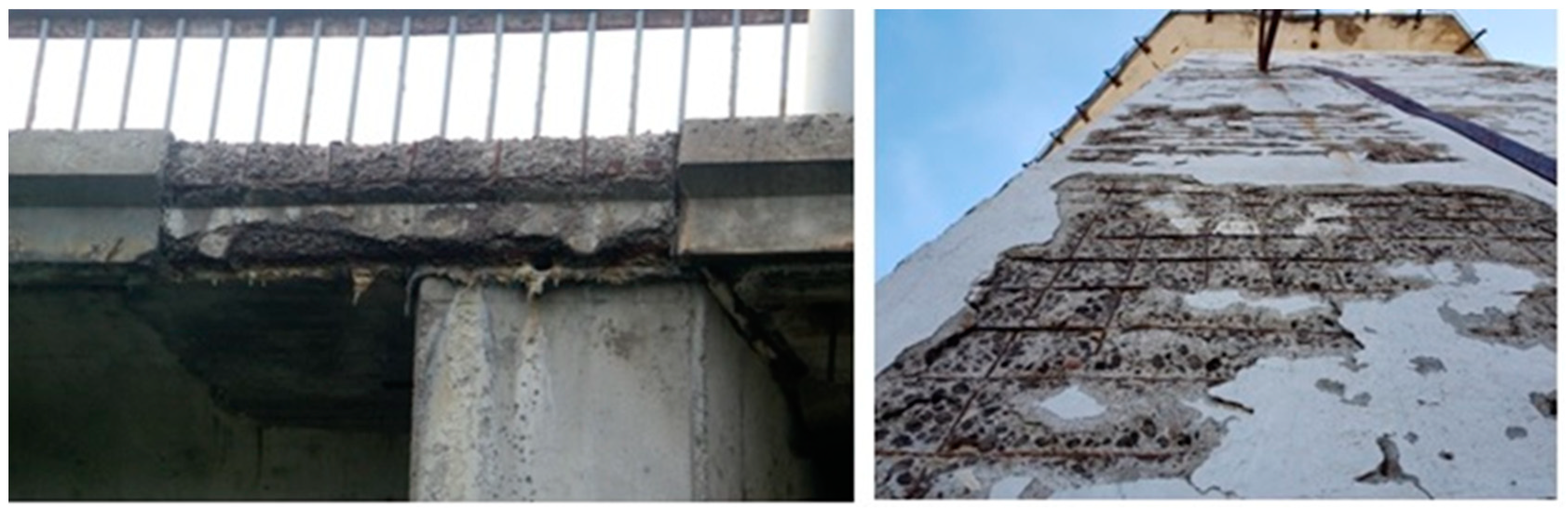
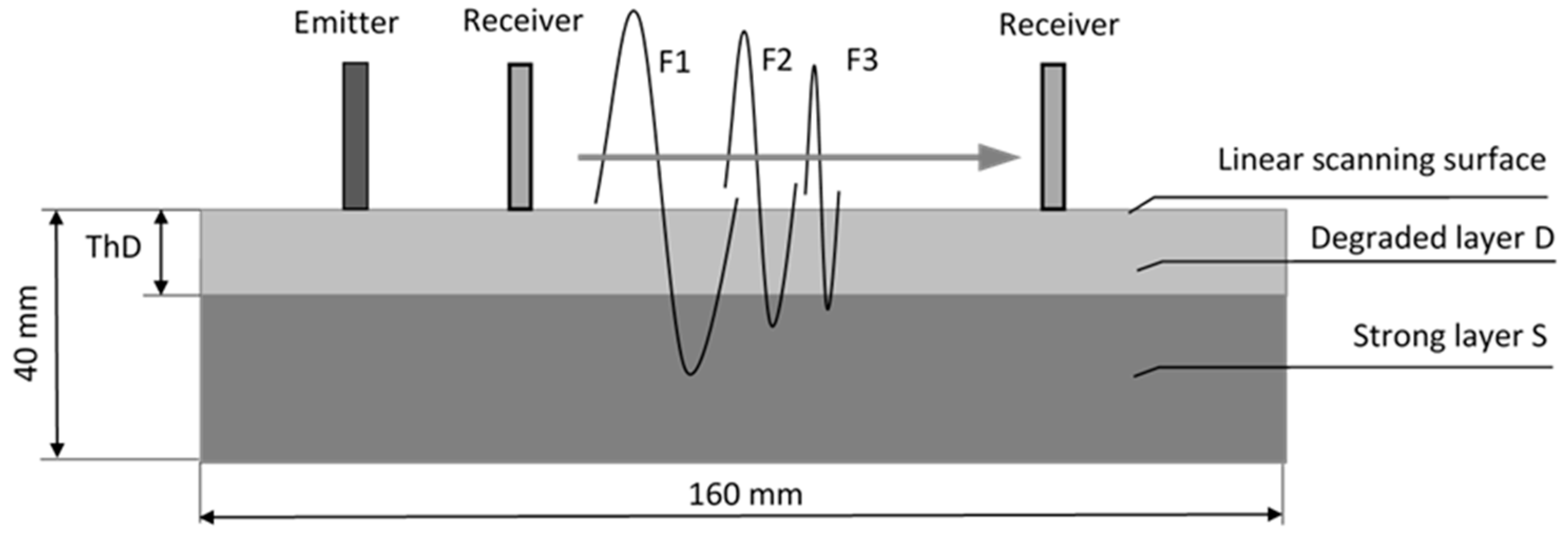
2.1. Concrete Specimens Modeling Degradation of Surface Layer

The specimens’ design corresponded to the purpose of this study—to explore the possibility of predicting two factors of interest describing the process of the deterioration of the concrete surface layer—the degree of the material degradation (D) and the depth or thickness of the degraded layer (ThD—Thickness of Degradation). Both of these factors were modeled in this simulation study. Two-layered concrete specimens with gradually varied D and ThD were intended for ultrasonic surface scanning at three ultrasonic frequencies (Figure 2). Conventionally “weak” and “strong” concretes simulated the upper degraded layer and the intact base layers, correspondingly, where the state of the concrete material was determined by changing the cement-to-sand ratio. The set of specimens created a two-dimensional data grid for constructing a mathematical model to recognize the two factors of interest, D and ThD.
Three stages of the conditionally “weak” surface layer, D1, D2 and D3, were selected, where the cement-to-sand ratios were 1:4 for D1, 1:7 for D2, and 1:12 for D3. The cement-to-sand ratio in the “strong” base layer S was 1:3. To select and indirectly estimate the strength of concrete mixtures for the solid and deteriorated layers, the ultrasound pulse velocity or the longitudinal wave velocity was preliminarily measured in homogeneous specimens with different cement-to-sand ratios using flat transducers at 100 kHz applied to the specimens’ facets. The measured values of the ultrasonic pulse velocity varied from 4400 m/s in the S layer to 2150 m/s in the D3 layer. Based on the empirical dependence of the velocity on the compressive strength taken from the available literature [51], the strength of the layers was approximately evaluated as 36 MPa for S, 25 MPa for D1, 14 MPa for D2, and 8 MPa for D3. The specimens were two-layer rectangular prisms of 160 × 40 × 40 mm with the degraded surface layer D and the base solid layer S. The thickness of the D layer ThD had 9 gradations, 0, 3, 5, 12, 20, 25, 30, 35 and 40 mm, where the specimens with ThD = 0 and ThD = 40 mm completely consisted of solid layer S and degraded layer D, respectively. To make the layers in the two-layer specimens adherent, the freshly prepared cement masses were poured sequentially—the top layer onto the bottom. To ensure proper adhesion, the top layer was lightly compacted. To avoid the effects of coarse aggregates on the result, a fine-grained filler was used with the largest fraction size not exceeding 3 mm. This is smaller than the thickness of the thinnest layer and the length of the ultrasonic wave at any frequency. Thus, the total number of specimens in the experiment was 27 (9 ThD grades and 3 D grades).

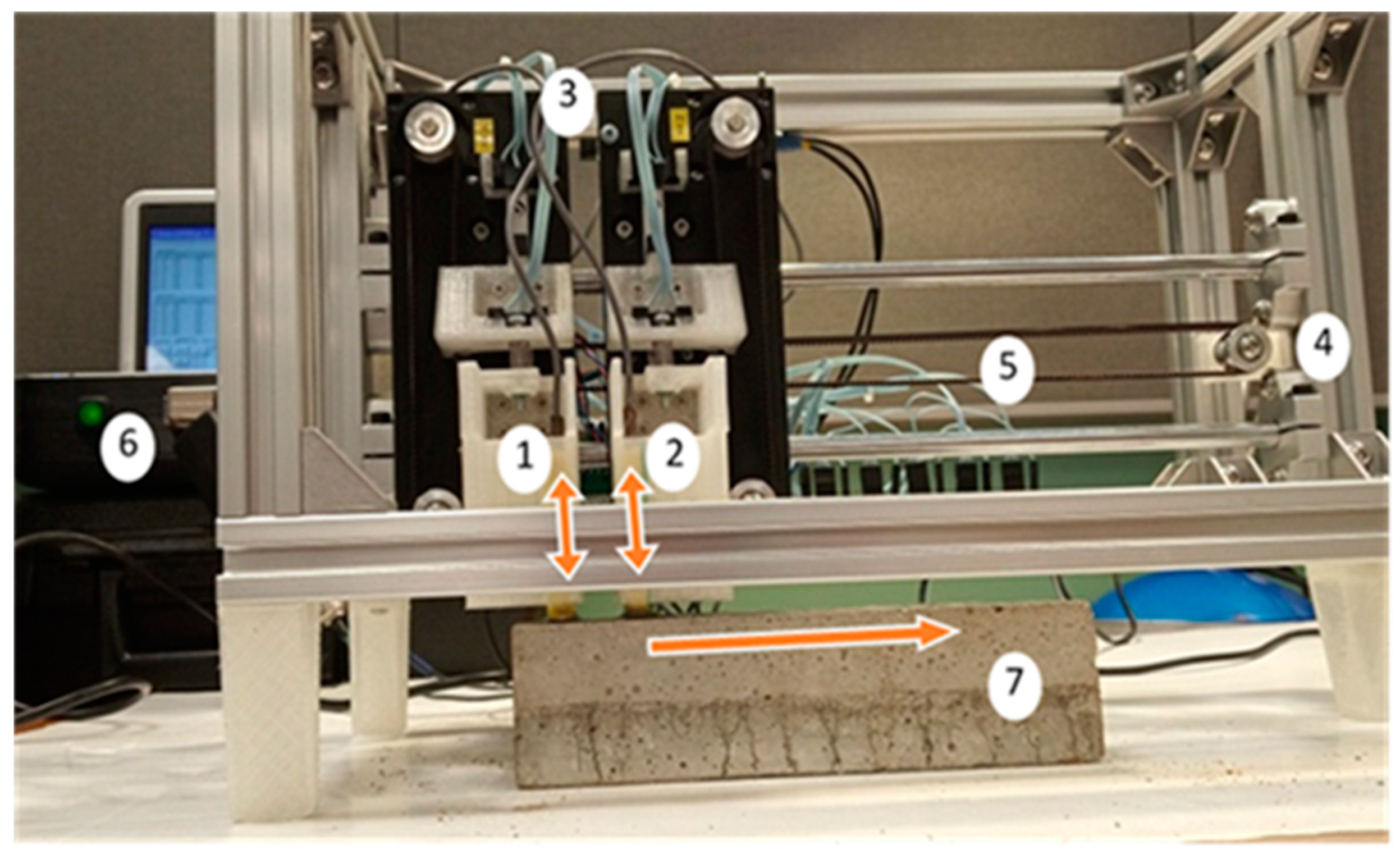
2.2. Ultrasonic Data Acquisition

To ensure rapid automated data collection and ultrasonic signal acquisition through stepwise surface profiling, a special scanning setup was developed, which included both a mechatronic scanning device and an electronic unit for ultrasonic data collection, synchronized in operation.
The main purpose of the scanning device (Figure 3) was the computer-aided positioning of piezoelectric transducers on a concrete specimen, which could have an inclined and uneven surface. The scanner had one horizontal axis for linear scanning and two parallel vertical axes for lifting and placing the transducers, each driven by stepper motors. The specimen was positioned under a fixed emitting transducer, and the motor drive moved the receiving transducer in a straight line on the specimen’s surface, changing the distance or acoustic base between the transducers in the range from 0 to 150 mm with an accuracy of 0.1 mm. The distance was read by the motor control program after preliminary calibration. Motor-driven vertical displacement of both the emitting and receiving transducers allowed them to be vertically positioned and pressed against the specimen’s surface with a dosed contact force set by preloading the spring. The scanner was designed as a frame made of aluminum profiles with all components mounted inside it. The mechatronic system consisted of a linear rod and rail movement system with a belt drive and NEMA series hybrid stepper motors NEMA11 and NEMA14 (MS Technology Co, Nanjing, China). The custom parts were manufactured from PLA plastic filament using an FDM 3D printer da Vinci Mini W+ (XYZPrinting, Taiwan). Repeatable positioning was provided by optical limit switches on each vertical axis, which defined the “home” position of the device. In addition, optical contact switches on the vertical axes indicated the contact of the transducers with the specimen’s surface. Motion control was performed by a single-board GRBL open source controller, which is a CNC Controller MKS DLC V2.1 (Guangzhou Makerbase Industry Co., Guangzhou, China) receiving G-code commands from a PC via USB. The pre-scan option was intended to obtain data on the specimen’s relief and take it into account during the main test. With a speed of movement of the sensors over the object of 2 points per second, taking into account the time for adaptive contact, the total scanning time of the specimen was about 12 s.
The purpose of ultrasonic acquisition was to collect a representable number of signals forming a so-called 2D spatiotemporal waveform profile or a digital 3D matrix composed of ultrasonic signals in the amplitude–time domain versus the step of scanning in the distance scale. A pair of identical emitter–receiver transducers was applied for signal acquisition in the pitch–catch mode in the surface transmission. The active elements of the transducers were piezoelectric plates of L × W × T = 20 × 4 × 1 mm, and the ultrasonic frequencies used corresponded to its flexural resonances. The plane of the sensors was parallel to the surface of the sample, and their long side was perpendicular to the direction of sounding. Thus, the size of the transducer in the direction of propagation of the ultrasonic wave was significantly smaller than the wavelength, which allowed the emitter to be considered quasi-pointing in this direction. A silicone-based acoustic gel was used as a coupling medium. To obtain ultrasonic responses containing wave modes with different wavelengths and the related different penetration depths, a set of three ultrasonic frequencies was applied: 50, 100 and 200 kHz. The choice of frequencies accounted for the intrinsic spectral characteristics of the transducers and the band of ultrasound propagation in concrete that is limited by a low kilohertz range. To enhance the dominance of the selected ultrasonic frequency, the excitation signal was tone-burst at this carrier frequency. The acquisition parameters are listed in Table 1.
The acquisition was controlled by custom-made circuitry (Figure 4) based on a field-programmable gate array (FPGA) chip Altera Cyclone IV EP4CE22E22C8 interacting with the exchange of commands and data with a computer through a USB 3.0 to FIFO interface bridge chip FT600Q. FPGA managed the output amplifier—a HV pulsar HV7360 microchip that provided emitting of ultrasonic tone-busts with output voltage up to 200 V peak-to-peak. Received ultrasonic signals were passed through a voltage gain amplifier (VGA) AD8367ARUZ of Analogue Devices with a voltage gain of up to 45 dB and digitized by ADC LTC2250, that is, a 10-bit 125 Msps/105 Msps low-noise analog-to digital converter of Linear Technology designed for digitizing high-frequency and wide-dynamic-range signals. High and low voltages in the circuitry were provided by a LT8331 DC/DC converter of Analogue Devices.
The processing core of FPGA managed the streams of transmitting and receiving data in FIFO buffering memory registers and additional buffers for digitized received signals and transmitted waveforms. State machine controllers provided synchronization between input and output signals. The ultrasonic data acquisition software developed in Microsoft Visual Studio using C++ processed the received data at a rate of 120 MB/s in real time and simultaneously performed data packaging, averaging and sorting. It had a complex multi-threaded scheme with 32 independent input threads in Pipeline mode, reading 1 MB of data packets and rewriting them into a common intermediate FIFO buffer. A separate thread averaged the data and placed them in the buffer memory for visualization and storage.

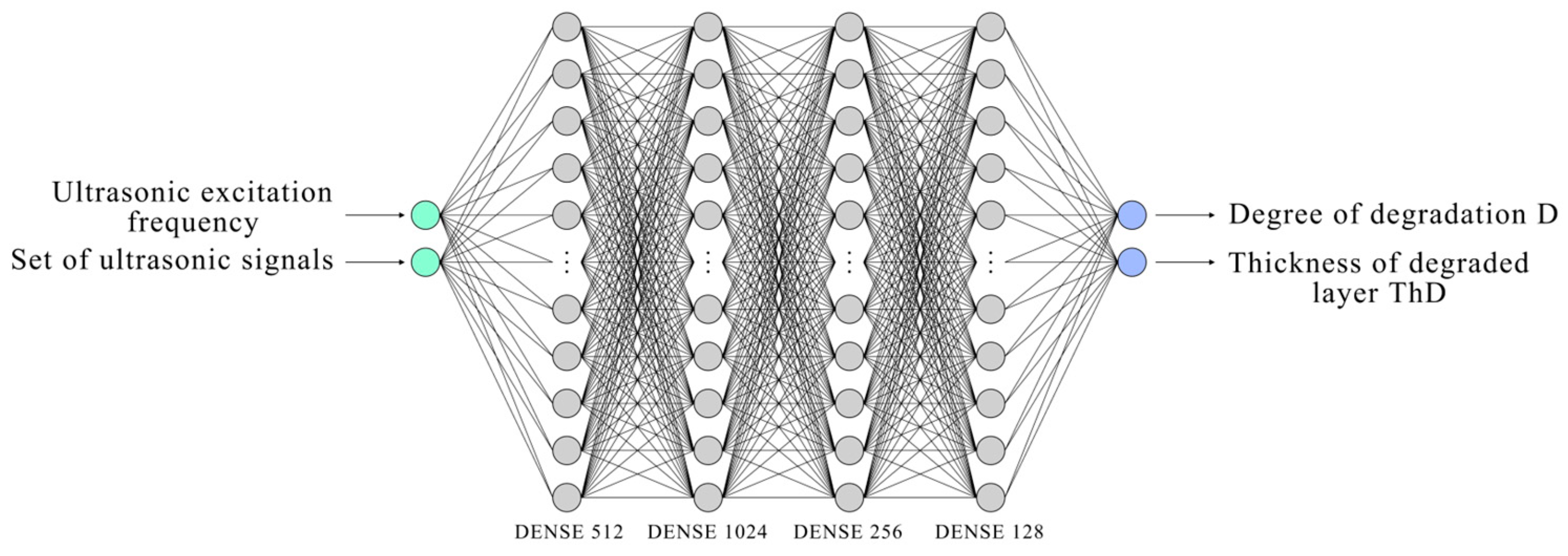
2.3. Building Neural Networks Based on Signals Obtained During Ultrasonic Measurements on the Surfaces of Concrete Specimens

Based on the results of ultrasound scanning, several neural networks were built to determine the degradation class {D1, D2, D3} and the depth of degradation of the concrete specimen ThD. The type of the created neural networks was a multilayer perceptron. Stochastic gradient descent was chosen as the learning algorithm. The architecture of the neural network is shown in Figure 5. It contains 4 hidden fully connected layers with the activation functions “ReLU” and “SoftMax” with 512, 1024, 256 and 128 elements, respectively. In addition to the hidden layers, the networks contain one input and one output layer. The input layer consists the elements with two components—a frequency in kilohertz and an array consisting of a set of measurements on the surface of each specific sample at 21 points. For each point, the measurement array contains 32,768 values, i.e., 688,128 values for 21 points. The output layer also contains two elements: the degree of degradation (D1, D2, D3) and the thickness of the upper weak layer ThD in millimeters. The neural network was trained on 100 epochs with validation. To achieve the best recognition rate, the weight characteristics of the hidden layers were normalized.
As described in paragraph 2.1, 27 concrete specimens were produced. The diagram describing the structure of the specimens is shown in Figure 6. The specimens differed in the thickness of the upper layer ThD (0, 3, 5, 12, 20, 25, 30, 35, 40 mm) and had 3 degrees of properties degradation: D1, D2 and D3. In each specimen, measurements were carried out at 3 frequencies. Thus, the dataset for building neural networks consisted of 81 elements. The dataset was divided into test, training and validation. The test dataset consisted of 18 elements (3 frequencies, 3 degrees of degradation D, 2 ThDs: 3 and 25 mm). The specimens used to create the test group, with ThDs of 3 and 25 mm and three degrees of degradation D, were located inside the range of the training group and marked in Figure 6 with white circles. The remaining dataset consisted of 63 elements. To prevent possible errors or dependencies related to the order of the data, the specimens were randomly shuffled and then divided into two parts: one for training, the other for validation. The training dataset consisted of 57 elements, and the validation dataset consisted of 6 elements. To evaluate the performance of the created neural networks, the following parameters were used: categorical cross-entropy was chosen as the loss function for the classification output, and mean squared error was used for the calculated parameter.

3. Results

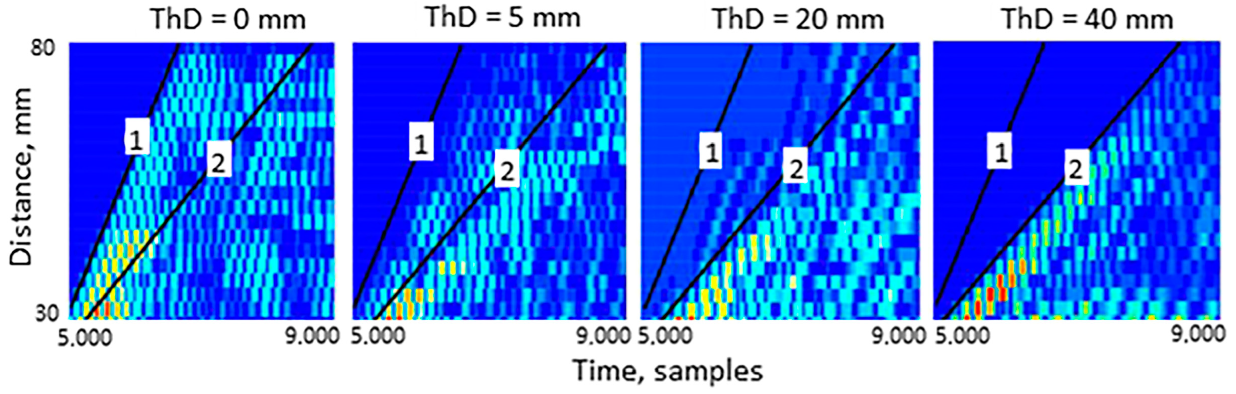
3.1. Spatiotemporal Waveform Profiles

Spatiotemporal waveform profiles were acquired by step-by-step scanning of specimens by a line in the middle of its upper surface. The distance between the transmitter and receiver was 20 mm at the starting point and then increased stepwise in 5 mm increments up to 120 mm. Thus, ultrasonic signals in 21 points of scanning of the 100 mm plot formed a set of ultrasonic signals or a spatiotemporal waveform profile to present it as a pattern of propagating ultrasonic waves. The spatiotemporal waveform profiles were consequently obtained at three excitation frequencies, 50, 100 and 200 kHz, where the excitation waveform was a two-period sine of the carrier frequency under a half-period sine envelope. Examples of typical recorded ultrasonic signals at three excitation frequencies and spatiotemporal waveform profiles, where the signals are presented as lines in the scanning steps consequence in the grey-scale brightness mode, are shown in Figure 7. For ease of presentation and mathematical processing of data, the time scale was presented as data points or time samples, where at a sampling rate of 30 MHz, the division value of one sample was equal to 0.033 microseconds.
The profiles presented complicated acoustic patterns with the interference of waves of various types, both direct propagation and reflected from the edges and facets of the specimen. In direct propagation, the following wave types can be distinguished by their prominent propagation patterns: fast propagating longitudinal or so-called “head” waves with the fastest arrival and slow-type waves of larger amplitude similar to surface Rayleigh waves. In monolithic specimens consisting of one layer, where ThD was zero (strong layer S) or maximum 40 mm (degraded layer D), the Rayleigh wave propagation graphs at its peak were linear at all three frequencies. This made it possible to measure the wave velocities as the distance-to-time ratio in the linearly approximated time-distance traces of first peaks in spatiotemporal waveform profiles (Figure 7). The obtained wave velocities (Table 2) confirmed a gradual decrease in the quality of the material from stage S to stage D3 in the projected sequence. However, knowledge of only the surface wave velocity is insufficient for the differential assessment of two factors of interest—the degree of degradation D and the layer thickness ThD. In addition, in the other specimens of the two-layer structure, the patterns of the spatiotemporal waveform profiles (Figure 8) were more complicated, which made it difficult to calculate wave velocities using peak traces. That is why, since the profiles contain information about the influence of both factors, neural network algorithms were used for their extraction.
However, in two-layered specimens, the wave pattern became more sophisticated due to splitting and interference of waves, propagating in the layers with different amplitudes. An example of the transformation of a spatiotemporal waveform profile at an ultrasonic frequency of 100 kHz with the increase in the thickness of the degraded layer ThD for case D3 is shown in Figure 8.
The following effect is observed: In the strong layer S (ThD = 0), the energy of the ultrasonic wave is concentrated near the wave front (line 1 in Figure 8), corresponding to propagation in this layer. In the monolithic specimen with degraded properties D3 (ThD = 40 mm), the energy of the ultrasonic wave is also concentrated near the wave front (line 2) but with a delay corresponding to a significantly lower wave velocity in the degraded material (see Table 2). Intermediate states with the presence of the upper degrading layer D and a lower strong layer S are characterized by a successive decrease in signal intensity between lines 1 and 2 with an increase in ThD, i.e., the depth of material degradation.
On one hand, these effects, demonstrating the dependence of successive changes in profiles on the ratio of the elastic properties of layers S and D and the thickness of layer D, suggest the possibility of using them for diagnostics. On the other hand, the complexity of the wave pattern, the presence of different acoustic modes and the interference of direct propagation signals with multiple reflections make it difficult to accurately predict the factors of interest analytically using any derived quantitative parameters. The use of neural networks made it possible to solve the task.

3.2. Application of NN

3.2.1. Classification Results for Ultrasonic Signals

To create the first neural network called “NN”, the entire array of available measurements was used, i.e., the values of the signal amplitude proportional to the surface stress and displacement for the entire time range in which ultrasound scanning was performed, i.e., from 1 to 32,768 time samples. Thus, the total length of the considered plot was equal to about 1 millisecond of real time at a 30 MHz sampling rate.
During the training of the neural network models, appropriate loss functions [52] were employed to minimize the error between the predicted and actual values. For regression tasks, such as predicting the thickness of the degraded layer (ThD), the mean squared error was used as the loss function.
M S E = 1 N i = 1 N y i y i 2
where y i is the actual value, y i is the predicted value, and N is the number of samples. This function penalizes larger deviations between the predicted and actual values, ensuring that the model learns to make accurate predictions.
For classification tasks, such as determining the degradation index (D1, D2, D3), the categorical cross-entropy loss function was used:
C C E = 1 N i = 1 N j = 1 C y i j log y i j
where y i j is a binary indicator (1 if the class label j is the correct class for sample i , 0 otherwise), y i j is the predicted probability for class j , and C is the total number of classes. This function ensures that the model maximizes the likelihood of assigning the correct class to each input sample.
The total loss function T o t a l   L o s s = α M S E + β C C E in the model combines the losses from the regression and classification tasks to ensure that both objectives are optimized simultaneously. This approach balances the contributions of each task during training. α and β are weighting coefficients that control the relative importance of the regression and classification tasks, respectively.
Table 3 (column 4, 5) shows the results of the neural network “NN” for the test dataset. After training, the total loss was 0.1165, the classification loss was 0.0799, and the loss for thickness estimation was 0.3654. As can be seen in Table 3 (columns 4 and 5), the degree of degradation was determined incorrectly only for 2 of 18 elements. The maximum relative error in determining the thickness was sufficiently large only in the case of a thin layer D with a thickness of 3 mm (Figure 9a). For the layer D, which is 25 mm thick, the thickness ThD is determined quite well—the relative error does not exceed 10% (Figure 9b).
To improve the prediction quality of the neural network, it was decided to take only the informative part of the ultrasonic signal, cutting off the initial area when the surface wave had not yet been formed, and the later part, which was formed mainly by the interference of reflected waves. To create the “NN3000“ network, different time ranges were selected for each frequency based on the constructed spatiotemporal waveform profiles (Figure 8): from 5000 to 10,000 samples for a frequency of 50 kHz, from 5000 to 9000 samples for a frequency of 100 kHz, and from 5000 to 8000 samples for a frequency of 200 kHz.
The type of neural network, architecture and learning process were not changed in relation to the already-created neural network “NN”. After training, the total loss was 0.1235, the loss for classification was 0.055 and the loss for thickness determination was 0.192. Classification statistics are shown in Table 3 (columns 6 and 7). After changing the input data, the network correctly predicted the degree of degradation D for all 18 elements of the test dataset, and the errors in determining the thickness of the upper layer ThD decreased (Figure 9). Thus, in the case of an upper layer with a thickness of 25 mm, the relative error did not exceed 4% (Figure 9b). This proves that in order to build a network, it is necessary to adjust the measurement range to the most informative one.
Since the result of network training improves with the increase in the training dataset, it was decided to take a wider range of signal propagation times (from 4000 to 14,000 samples) and the same for all the frequencies considered. Thus, 10,000 measured values were taken into account for each of the 21 points at which measurements were carried out. The neural network built on the basis of these data was named “NN10000”. The types of neural network, architecture and learning process were the same. After training, the total loss was 0.115, the loss for classification was 0.0535 and the loss for thickness determination was 0.0615. The classification statistics are given in Table 3 (columns 8 and 9).
Table 3 shows that the “NN10000” network also correctly predicted the degree of degradation D for all 18 elements of the test dataset, while the errors in determining the thickness ThD decreased slightly (Figure 9). In the case of the thickness ThD 25 mm, the relative error now did not exceed 3% (Figure 9b). In general, the quality of the results of the “NN3000” and “NN10000” networks differs insignificantly, indicating that the number of training data was quite sufficient to obtain acceptable results.

3.2.2. Classification Results for Ultrasonic Signals in Frequency Domain After FFT

Fourier amplitude spectra were constructed for the signals obtained during measurements on the surfaces of concrete specimens. In signal processing, the Fourier transform is the most popular tool for signal conversion from the time domain to the frequency domain [53]. The types of neural networks, architecture and learning process were not changed in relation to the already-created neural networks. Similarly to the “NN”, “NN3000” and “NN10000” networks, the “NNFT”, “NNFT3000” and “NNFT10000” networks were constructed. The frequency and array of amplitude spectrum values were taken as input data for the new networks instead of signals for similar time ranges. For the NNFT network, after training, the total loss was 0.287, the loss for classification was 0.174 and the loss for thickness determination was 0.113. The classification statistics are given in Table 4 (columns 4 and 5).
For “NNFT10000”, after training, the total loss was 0.245, the loss for classification was 0.0913 and the loss for thickness determination was 0.1537. The classification statistics are given in Table 4 (columns 6 and 7). For “NNFT3000”, after training, the total loss was 0.2763, the loss for classification was 0.0874 and the loss for thickness determination was 0.1889. The classification statistics are given in Table 4 (columns 8 and 9).
As the results collected in Table 4 show, neural networks that use Fourier amplitude spectra rather than the signals themselves do not determine the factors of interest so well. Errors occur when determining the degree of degradation, in some cases up to two gradations of D. Errors in determining the thickness ThD become significantly higher (Figure 10).
The Fourier amplitude spectrum does not contain information about the signal change in the time scale. It indicates which frequencies are reproduced, but the time points at which these frequencies appear are not recognized. Abrupt changes and local fluctuations in the signal, as well as the beginnings and ends of such bursts, are not detected by the Fourier transform. As is shown in Figure 8, the spatiotemporal waveform profiles obtained over the surface of concrete specimens in the time domain depend on the thickness ThD. After applying the Fourier transform, information about this time dependence is partially lost and the quality of neural network predictions deteriorates. It would be possible to try to apply a processing tool like the wavelet transform that gives a time-frequency description of the signal. However, since neural networks built on the basis of raw signals themselves allow determining the thickness of the degraded layer ThD with sufficient accuracy and accurately determining the degree of degradation D, there is no need to modify them additionally.
As is evident from the comparison of detection errors at three excitation frequencies and for different time ranges of signals presented in Table 3 and Table 4 and Figure 9 and Figure 10, the smallest total number of errors in determining the degree of degradation D and the best accuracy in determining the thickness ThD were obtained for excitation at a frequency of 200 kHz in the NN10000 range. This may seem to contradict the idea that at a frequency of 50 kHz, where the wavelength and, accordingly, the depth of penetration of the ultrasound surface wave into the specimen are 4 times greater, the prediction accuracy should be higher, especially for large values of ThD. This can be explained by the dependence of the penetration depth of the Rayleigh surface wave into the material on the wavelength and, consequently, on the frequency [14]. The lower the frequency, the greater the wavelength and the wave’s penetration depth. Thus, for the recognition of ThD at large ThD values, a low frequency (in our case 50 kHz) would be preferable. However, when comparing the actual spectra of ultrasonic signals at three excitation frequencies, examples of which are shown in Figure 11, it turned out that at 200 kHz, the signals also contain a low-frequency component with a frequency of 50 kHz, whereas with excitation of 50 kHz, no harmonics are observed at higher frequencies. Thus, it is possible to establish that the best degree of recognition of factors of interest by the method of neural network analysis can be obtained using signals with a rich spectrum, containing both low-frequency and high-frequency components. When changing ThD in a wide range, a positive recognition effect is achieved using surface waves with a wide range of wavelengths and penetration depths, correspondingly. It is also necessary to choose an optimal informative time range of signals, which would contain, if possible, all acoustic modes of direct propagation, but which at the same time would be free from parasitic components related to multiple reflections and reverberations (case NN10000 in our experiment).

4. Conclusions

This study showed the possibility of creating an artificial intelligence system to predict changes in both parameters of deterioration of the surface layer of concrete—the degree of degradation of the material and the thickness (depth) of the degraded layer. This became possible due to using ultrasonic spatiotemporal waveform profiles or consequences of step-by-step acquired ultrasonic signals for various frequencies obtained by surface profiling. It was proven that the volume of input data used was sufficient to successfully train the created neural network model and to obtain good results in determining the parameters of the degradation of concrete.
The parts of the signals that were most sensitive to changes in the factors of interest were identified. Using only such significant regions of spatiotemporal profiles made it possible to significantly improve the neural networks built on this basis. It was demonstrated that the most accurate prediction was obtained using ultrasonic signals with the widest spectral response, where the main frequency components of the signal were maximally spaced over the frequency scale.
The obtained measurement data were processed with the help of discrete Fourier transform, and amplitude spectra were constructed. The spectra were also analyzed with created artificial neural networks. The obtained results in the frequency domain demonstrated worse prediction accuracy than the results of neural networks built on the basis of raw ultrasonic signals in the time domain. The disadvantage of the Fourier transform is the lack of localization property: if the signal changes in a certain time interval, then the transformed signal (amplitude spectrum) changes everywhere, and it is impossible to determine the time of change in the original signal. In this case, information about the temporal characteristics of signal propagation, which are the propagation velocities of various acoustic modes in the layers, is lost. In contrast, it is the velocity of ultrasonic waves that reflects the quality of the concrete material in terms of its elastic properties and strength.
To improve the accuracy of the method in further studies, the following measure can be proposed: building a mathematical prediction model based on a larger amount of experimental data in the training set with more detailed filling of intermediate conditions; extensive simulations are required to create training, control and test data for different parameters. Therefore, another goal is the creation of simulation models for the rapid calculation of wave propagation in gradient materials.
From the point of view of practical application, further research can be aimed at constructing prediction models in real concrete structures subject to destructive action of the environment, such as concretes under freeze–thaw cycles and refractory concretes.
Deteriorated concrete is characterized by the heterogeneity of properties and can be considered as a gradient material. Gradient materials more and more are being used for many important industries. The gradient can be categorized as either continuous or discontinuous, which exhibits a stepwise gradient [54]. Still, only partial problems are solved in the determination of the stiffness gradients using ultrasonic waves [55]. So far, projection methods for solving inverse problems have been developed only for the two-dimensional case and for selected forms of material property change [56]. Therefore, the development of methods for monitoring the material properties of gradient materials remains a current task. A comprehensive assessment of the condition requires the development of new diagnostic approaches and the use of sophisticated data processing, in particular the use of artificial intelligence methods that can provide smarter and more efficient new approaches for this. In this work, the properties of gradient concrete structures were investigated using artificial intelligence methods.
This work presents an original approach demonstrating the possibilities of assessing simultaneously two factors of interest, describing the process of deterioration of the surface layer of the material by depth—at what degree the material degraded in its physical properties (strength, toughness) and to what depth these changes spread. Such a complex assessment of two factors as applied to the deterioration processes in concrete degradation using surface acoustic waves and ANN has not yet been demonstrated.

Author Contributions

Conceptualization, E.K. and A.T.; methodology, E.K. and A.T.; software, S.K. and G.S.; validation, S.K. and G.S.; formal analysis, A.T. and E.K.; investigation, S.K.; resources, G.S.; data curation, S.K. and A.T.; writing—original draft preparation, E.K., A.T. and G.S.; writing—review and editing, E.K., A.T. and G.S.; visualization, A.T. and S.K.; supervision, E.K. and A.T.; project administration, E.K. and A.T.; funding acquisition, E.K. and A.T. All authors have read and agreed to the published version of the manuscript.

Funding

This research was funded by the grant 40170133 of the RheinMain University of Applied Sciences, Wiesbaden, Germany, as part of a study on artificial neural networks and by the grant lzp-2020/2-0033 of the Latvian Council of Science as part of a ultrasonic data acquisition project.

Data Availability Statement

The original contributions presented in this study are included in the article. Further inquiries can be directed to the corresponding author.

Conflicts of Interest

The authors declare no conflicts of interest.

References

  1. Breugel, K. Societal burden and engineering challenges of ageing infrastructure. Procedia Eng. 2017, 171, 53–63. [Google Scholar] [CrossRef]
  2. Hobbs, D.W. Concrete deterioration: Causes, diagnosis, and minimising risk. Int. Mater. Rev. 2001, 46, 117–144. [Google Scholar] [CrossRef]
  3. Rosenqvist, M.; Pham, L.-W.; Terzic, A.; Fridh, K.; Hassanzadeh, M. Effects of interactions between leaching, frost action and abrasion on the surface deterioration of concrete. Constr. Build. Mater. 2017, 149, 849–860. [Google Scholar] [CrossRef]
  4. Bahafid, S.; Hendriks, M.; Jacobsen, S.; Geiker, M. Revisiting concrete frost salt scaling: On the role of the frozen salt solution micro-structure. Cem. Concr. Res. 2022, 157, 106803. [Google Scholar] [CrossRef]
  5. ElKhatib, L.W.; Khatib, J.; Assaad, J.J.; Elkordi, A.; Ghanem, H. Refractory Concrete Properties—A Review. Infrastructures 2024, 9, 137. [Google Scholar] [CrossRef]
  6. Malaiškienė, J.; Antonovič, V.; Boris, R.; Kudžma, A.; Stonys, R. Analysis of the Structure and Durability of Refractory Castables Impregnated with Sodium Silicate Glass. Ceramics 2023, 6, 2320–2332. [Google Scholar] [CrossRef]
  7. Schabowicz, K. Non-destructive testing of materials in civil engineering. Materials 2019, 12, 3237. [Google Scholar] [CrossRef]
  8. Khan, A.A. Guidebook on Non-Destructive Testing of Concrete Structures; Training Courses Series; IAEC (International Atomic Energy Agency): Vienna, Austria, 2002; Volume 17. [Google Scholar]
  9. Kundu, T. (Ed.) Ultrasonic Non-Destructive Evaluation Engineering Biological Material Characterization; CRC Press: Boca Raton, FL, USA, 2003; 848p. [Google Scholar]
  10. Komlos, K.; Popovics, S.; Niirnbergeroh, T.; Babd, B.; Popovics, J.S. Ultrasonic pulse velocity test of concrete properties as specified in various standards. Cem. Concr. Compos. 1996, 18, 357–364. [Google Scholar] [CrossRef]
  11. Lencis, U.; Udris, A.; Kara De Maeijer, P.; Korjakins, A. Methodology for determining the correct ultrasonic pulse velocity in concrete. Buildings 2024, 14, 720. [Google Scholar] [CrossRef]
  12. Irrigaray, M.A.P.; Pinto, R.; Padaratz, I.J. A new approach to estimate compressive strength of concrete by the UPV method. Rev. IBRACON De Estrut. E Mater. 2016, 9, 395–402. [Google Scholar] [CrossRef]
  13. Chakraborty, J.; Wang, X.; Stolinski, M. Analysis of sensitivity of distance between embedded ultrasonic sensors and signal processing on damage detectability in concrete structures. Acoustics 2022, 4, 89–110. [Google Scholar] [CrossRef]
  14. Victorov, I.A. Rayleigh and Lamb Waves. Physical Theory and Applications; Plenum Press: New York, NY, USA, 1967. [Google Scholar]
  15. Li, M.; Anderson, N.; Sneed, L.; Maerz, N. Application of ultrasonic surface wave techniques for concrete bridge deck condition assessment. J. Appl. Geophys. 2016, 126, 148–157. [Google Scholar] [CrossRef]
  16. Cho, Y.S. Non-destructive testing of high strength concrete using spectral analysis of surface waves. NDTE Int. 2003, 36, 229–235. [Google Scholar] [CrossRef]
  17. RILEM NDT 4, Recommendation for In Situ Concrete Strength Determination by Combined Non-Destructive Methods, Compendium of RILEM Technical Recommendations; E&FN Spon: London, UK, 1993.
  18. Tatarinov, A.; Sisojevs, A.; Chaplinska, A.; Shahmenko, G.; Kurtenoks, V. An approach for assessment of concrete deterioration by surface waves. Procedia Struct. Integr. 2022, 37, 453–461. [Google Scholar] [CrossRef]
  19. Li, M.; Salucci, M. Applications of Deep Learning in Electromagnetics: Teaching Maxwell’s Equations to Machines; IET Digital Library: Stevenage, UK, 2022; 480p. [Google Scholar] [CrossRef]
  20. Bowler, A.L.; Pound, M.P.; Watson, N.J. A review of ultrasonic sensing and machine learning methods to monitor industrial processes. Ultrasonics 2022, 124, 106776. [Google Scholar] [CrossRef]
  21. Goodfellow, I.; Bengio, Y.; Courville, A. Deep Learning; MIT Press Massachusetts Institute of Technology: Cambridge, MA, USA, 2016; ISBN 9780262035613. [Google Scholar]
  22. Chan, K.Y.; Abu-Salih, B.; Qaddoura, R.; Al-Zoubi, A.M.; Palade, V.; Pham, D.S.; Del Ser, J.; Muhammad, K. Deep neural networks in the cloud: Review, applications, challenges and research directions. Neurocomputing 2023, 545, 126327. [Google Scholar] [CrossRef]
  23. Hind, T.; Mas, J.-F. Multilayer Perceptron (MLP); In Geomatic Approaches for Modeling Land Change Scenarios; Springer: Cham, Switzerland, 2018. [Google Scholar] [CrossRef]
  24. Khotanzad, A.; Chung, C. Application of multi-layer perceptron neural networks to vision problems. Neural Comput. Applic. 1988, 7, 249–259. [Google Scholar] [CrossRef]
  25. Haykin, S. Neural Networks: A Comprehensive Foundation, 2nd ed.; Prentice Hall: Englewood Cliffs, NJ, USA, 1998; 842p, ISBN 978-0-13-273350-2. [Google Scholar]
  26. Abdi, H.; Williams, L.J. Principal component analysis. Wiley Interdiscip. Rev. Comput. Stat. 2010, 2, 433–459. [Google Scholar] [CrossRef]
  27. Salas-Gonzalez, D.; Górriz, J.M.; Ramírez, J.; Illán, I.A.; López, M.; Segovia, F.; Chaves, R.; Padilla, P.; Puntonet, C.G.; Alzheimer’s Disease Neuroimage Initiative. Feature selection using factor analysis for Alzheimer’s diagnosis using 18F-FDG PET images. Med. Phys. 2010, 37, 6084–6095. [Google Scholar] [CrossRef]
  28. Zhang, K.; Lv, G.; Guo, S.; Chen, D.; Liu, Y.; Feng, W. Evaluation of subsurface defects in metallic structures using laser ultrasonic technique and genetic algorithm-back propagation neural network. NDT E Int. 2020, 116, 102339. [Google Scholar] [CrossRef]
  29. Liu, J.; Xu, G.; Ren, L.; Qian, Z.; Ren, L. Defect intelligent identification in resistance spot welding ultrasonic detection based on wavelet packet and neural network. Int. J. Adv. Manuf. Technol. 2017, 90, 2581–2588. [Google Scholar] [CrossRef]
  30. Wang, Y. Wavelet transform based feature extraction for ultrasonic flaw signal classification. J. Comput. 2014, 9, 725–732. [Google Scholar] [CrossRef]
  31. Mousavi, M.; Taskhiri, M.S.; Holloway, D.; Olivier, J.; Turner, P. Feature extraction of woodhole defects using empirical mode decomposition of ultrasonic signals. NDT E Int. 2020, 114, 102282. [Google Scholar] [CrossRef]
  32. Waszczyszyn, Z.; Ziemianski, L. Neural networks in mechanics of structures and materials—New results and prospects of applications. Comput. Struct. 2001, 79, 2261–2276. [Google Scholar] [CrossRef]
  33. Liu, S.W.; Huang, J.H.; Sung, J.C.; Lee, C.C. Detection of cracks using neural networks and computational mechanics. Comput. Methods Appl. Mech. Eng. 2002, 191, 2831–2845. [Google Scholar] [CrossRef]
  34. Khandetsky, V.; Antonyuk, I. Signal processing in defect detection using back-propagation neural networks. NDTE Int. 2002, 35, 483–488. [Google Scholar] [CrossRef]
  35. Xu, Y.; Liu, G.; Wu, Z.; Huang, X. Adaptive multilayer perceptron networks for detection of cracks in anisotropic laminated plates. Int. J. Solids Struct. 2001, 38, 5625–5645. [Google Scholar] [CrossRef]
  36. Fang, X.; Luo, H.; Tang, J. Structural damage detection using neural network with learning rate improvement. Comput. Struct. 2005, 83, 2150–2161. [Google Scholar] [CrossRef]
  37. Hernández-Gómez, L.H.; Durodola, J.; Fellows, N.; Urriolagoitia-Calderón, G. Locating defects using dynamic strain analysis and artificial neural networks. Appl. Mech. Mater. 2005, 3–4, 325–330. [Google Scholar] [CrossRef]
  38. Shi, S.; Jin, S.; Zhang, D.; Liao, J.; Fu, D.; Lin, L. Improving Ultrasonic Testing by Using Machine Learning Framework Based on Model Interpretation Strategy. Chin. J. Mech. Eng. 2023, 36, 127. [Google Scholar] [CrossRef]
  39. Lv, G.; Guo, S.; Chen, D.; Feng, H.; Zhang, K.; Liu, Y.; Feng, W. Laser ultrasonics and machine learning for automatic defect detection in metallic components. NDT E Int. 2023, 133, 102752. [Google Scholar] [CrossRef]
  40. Ferreira, G.R.B.; Ribeiro, M.G.d.C.; Kubrusly, A.C.; Ayala, H.V.H. Improved feature extraction of guided wave signals for defect detection in welded thermoplastic composite joints. Measurement 2022, 198, 111372. [Google Scholar] [CrossRef]
  41. Solov’ev, A.N.; Cherpakov, A.V.; Vasil’ev, P.V.; Parinov, I.A.; Kirillova, E.V. Neural network technology for identifying defect sizes in half-plane based on time and positional scanning. Adv. Eng. Res. 2020, 20, 205–215. [Google Scholar] [CrossRef]
  42. Shrestha, A.; Mahmood, A. Review of deep learning algorithms and architectures. IEEE Access 2019, 7, 53040–53065. [Google Scholar] [CrossRef]
  43. Hu, T.; Zhao, J.; Zheng, R.; Wang, P.; Li, X.; Zhang, Q. Ultrasonic based concrete defects identification via wavelet packet transform and GA-BP neural network. PeerJ Comput. Sci. 2021, 7, e635. [Google Scholar] [CrossRef]
  44. Shin, H.K.; Ahn, Y.H.; Lee, S.H.; Kim, H.Y. Automatic concrete damage recognition using multi-level attention convolutional neural network. Materials 2020, 13, 5549. [Google Scholar] [CrossRef]
  45. Nyathi, M.A.; Bai, J.; Wilson, I.D. Deep Learning for Concrete Crack Detection and Measurement. Metrology 2024, 4, 66–81. [Google Scholar] [CrossRef]
  46. Rodrigues, L.F.M.; Cruz, F.C.; Oliveira, M.A.; Filho, E.F.S.; Albuquerque, M.S.C.; da Silva, I.C.; Farias, C.T.T. Identification of carburization level in industrial HP pipes using ultrasonic evaluation and machine learning. Ultrasonics 2018, 94, 145–151. [Google Scholar] [CrossRef]
  47. Almasaeid, H. Ultrasonic pulse velocity and artificial neural network prediction of high-temperature damaged concrete splitting strength. Discov. Appl. Sci. 2024, 6, 4. [Google Scholar] [CrossRef]
  48. Bonagura, M.; Nobile, L. Artificial Neural Network (ANN) Approach for Predicting Concrete Compressive Strength by SonReb. Struct. Durab. Health Monit. 2021, 15, 125–137. [Google Scholar] [CrossRef]
  49. Park, J.Y.; Yoon, Y.G.; Oh, T.K. Prediction of Concrete Strength with P-, S-, R-Wave Velocities by Support Vector Machine (SVM) and Artificial Neural Network (ANN). Appl. Sci. 2019, 9, 4053. [Google Scholar] [CrossRef]
  50. Wang, J.; Schmitz, M.; Jacobs, L.J.; Qu, J. Deep learning-assisted locating and sizing of a coating delamination using ultrasonic guided waves. Ultrasonics 2024, 141, 107351. [Google Scholar] [CrossRef] [PubMed]
  51. Trtnik, G.; Kavcic, F.; Turk, G. Prediction of concrete strength using ultrasonic pulse velocity and artificial neural networks. Ultrasonics 2009, 49, 53–60. [Google Scholar] [CrossRef] [PubMed]
  52. Terven, J.; Cordova-Esparza, D.-M.; Ramirez-Pedraza, A.; Chávez Urbiola, E. Loss Functions and Metrics in Deep Learning. A Review. arXiv 2024. [Google Scholar] [CrossRef]
  53. Stone, J.V. The Fourier Transform: A Tutorial Introduction; Sebtel Press, University of Shefield: Sheffield, UK, 2021; 91p. [Google Scholar]
  54. Li, Y.; Feng, Z.; Hao, L.; Huang, L.; Xin, C.; Wang, Y.; Bilotti, E.; Essa, K.; Zhang, H.; Li, Z.; et al. A Review on Functionally Graded Materials and Structures via Additive Manufacturing: From Multi-Scale Design to Versatile Functional Properties. Adv. Mater. Technol. 2020, 5, 1900981. [Google Scholar] [CrossRef]
  55. Lu, L.; Chekroun, M.; Abraham, O.; Maupin, V.; Villain, G. Mechanical properties estimation of functionally graded materials using surface waves recorded with a laser interferometer. NDT E Int. 2011, 44, 169–177. [Google Scholar] [CrossRef]
  56. Vatulyan, A.O.; Bogachev, I.V. The Projection Method for Identification of the Characteristics of Inhomogeneous Solids. Dokl. Phys. 2018, 63, 82–85. [Google Scholar] [CrossRef]
Figure 1. Examples of deterioration of concrete infrastructure objects progressing from the surface (data from the Latvian Concrete Association).
Acoustics 07 00019 g001
Figure 2. Two-layered concrete specimen with gradually varied thickness of degraded upper layer ThD intended for ultrasonic surface scanning using three frequencies F1–F3.
Acoustics 07 00019 g002
Figure 3. Ultrasonic scanner in action: 1—emitting transducer; 2—receiving transducer; 3—vertical position controls; 4—linear displacement drive; 5—PCB for scanning control; 6—ultrasonic acquisition unit; 7—double-layered concrete specimen. Vertical arrows show the attachment of the transducers; horizontal line shows the direction of the step-by-step linear displacement of the receiving transducer.
Acoustics 07 00019 g003
Figure 4. Principal diagram of ultrasonic acquisition circuitry.
Acoustics 07 00019 g004
Figure 5. NN architecture.
Acoustics 07 00019 g005
Figure 6. Structure of dataset: black circles represent specimens for training and validation, while empty circles represent specimens for testing.
Acoustics 07 00019 g006
Figure 7. Typical ultrasonic signals in a concrete specimen at 50, 100 and 200 kHz (left column) and spatiotemporal waveform profiles formed by step-by-step profiling of the specimen’s surface (right column), where 1 sample is equivalent 0.033 μs.
Acoustics 07 00019 g007
Figure 8. Changes in spatiotemporal waveform profiles at 100 kHz with gradual increase in thickness of degraded layer ThD in specimens from series with degradation degree D3: 1 and 2—wave front lines at ThD = 0 mm and ThD = 40 mm, correspondingly, where 1 sample is equivalent 0.033 μs.
Acoustics 07 00019 g008
Figure 9. Maximal for 3 degrees of deterioration-related relative errors for ThD (ANN for ultrasonic signals) (a) ThD = 3 mm. (b) ThD = 25 mm.
Acoustics 07 00019 g009
Figure 10. Maximal for 3 degrees of deterioration-related relative errors for ThD (for ultrasonic signals in frequency domain after FFT). (a) ThD = 3 mm. (b) ThD = 25 mm.
Acoustics 07 00019 g010
Figure 11. Spectra of typical ultrasonic signals at carrier excitation frequencies 50 (a), 100 (b), and 200 (c) kHz obtained by FFT: 1—using cut signal length as for “NN10000” analysis; 2—using entire signal length as for “NN” analysis; 3—carrier excitation frequency.
Acoustics 07 00019 g011
Table 1. Parameters of ultrasonic acquisition.
ParameterValue
Applied ultrasonic frequencies50, 100, 200 kHz
Excitation waveform2-period sine tone-burst
Output voltage100 V p-t-p
ADC of received ultrasonic signals10-bit, 30 MHz
Length and step of scanning100 mm, 5 mm
Number of ultrasonic signals in a profile set21
Table 2. Velocities of surface waves in monolithic specimens of S and D layers.
Ultrasonic Frequency, kHzVelocity, m/s
SD1D2D3
502287191616761266
1002300197817841278
2002353202017801318
Table 3. The classification statistics for the applied network for ultrasonic signals.
Ultrasonic Frequency, kHzProjected ValuesPredicted Values with Different Networks
“NN”“NN3000”“NN10000”
D,
Degree
ThD, mmD,
Degree
ThD, mmD,
Degree
ThD, mmD,
Degree
ThD, mm
50D13.0D3 **3.67D12.31D13.69
50D23.0D24.08D23.83D23.09
50D33.0D1 **3.99D32.91D32.44
100D13.0D13.34D12.36D13.50
100D23.0D23.44D22.60D23.56
100D33.0D32.53D33.91D33.06
200D13.0D12.84D13.40D12.80
200D23.0D23.94D23.45D22.84
200D33.0D32.94D33.40D33.60
50D125.0D123.64D125.98D125.65
50D225.0D225.32D224.99D224.63
50D325.0D327.87D325.73D325.76
100D125.0D126.44D124.60D124.84
100D225.0D227.00D225.04D224.27
100D325.0D325.67D325.34D324.50
200D125.0D127.26D125.85D125.19
200D225.0D227.09D225.66D225.42
200D325.0D324.70D324.53D324.29
**—deviation in D by 2 gradations.
Table 4. The classification statistics for the applied network for ultrasonic signals in frequency domain after FFT.
Ultrasonic Frequency,
kHz
Projected ValuesPredicted Values with Different Networks
“NNFT”“NNFT3000”“NNFT10000”
D,
Degree
ThD, mmD,
Degree
ThD, mmD,
Degree
ThD, mmD,
Degree
ThD, mm
50D13.0D2 *0.99D3 **3.92D14.99
50D23.0D23.67D22.83D24.09
50D33.0D1 **5.93D34.55D31.37
100D13.0D11.23D3 **3.36D11.80
100D23.0D3 *0.024D3 *4.34D21.87
100D33.0D31.86D34.92D34.09
200D13.0D13.95D3 **6.65D12.19
200D23.0D25.09D23.97D22.29
200D33.0D2 *5.98D34.87D2*4.37
50D125.0D122.32D128.73D123.66
50D225.0D3 *22.89D227.47D3*25.00
50D325.0D326.10D328.35D326.21
100D125.0D124.91D126.88D123.98
100D225.0D225.66D223.31D224.51
100D325.0D1 **22.69D328.12D1**24.55
200D125.0D126.75D128.20D123.92
200D225.0D223.42D228.55D224.47
200D325.0D326.58D325.34D324.29
*, **—deviation in D by 1 and 2 gradations, correspondingly.
Disclaimer/Publisher’s Note: The statements, opinions and data contained in all publications are solely those of the individual author(s) and contributor(s) and not of MDPI and/or the editor(s). MDPI and/or the editor(s) disclaim responsibility for any injury to people or property resulting from any ideas, methods, instructions or products referred to in the content.

