Impact of Motorway Speed Management on Environmental Noise: Insights from High-Resolution Monitoring

Abstract

This study explores the impact of road transport on the environment, focusing on noise pollution. Using high-resolution, one-minute data from a low-cost environmental sensor, this research examines traffic flow dynamics, meteorological influences, and their relationship to noise along a major transport corridor. The methodology combines cluster analysis and descriptive statistics to evaluate the effects of deploying a Smart Motorway Variable Speed Limit (SMVSL) system over a six-month monitoring period. Results indicate that SMVSL systems not only smooth traffic flow but also significantly reduce noise variability, particularly during peak hours, thus mitigating noise peaks associated with adverse health outcomes. LAeq values were found to differ modestly between day and night, with clustering revealing a reduction in extreme noise events (LAmax > 70 dB(A)) in SMVSL scenarios dominated by heavy goods vehicles. This study further identifies associations between unmanaged speed regimes and elevated noise levels, enriching our understanding of the environmental impacts of unregulated traffic conditions. These findings inform sustainable planning and policy strategies aimed at improving urban environmental quality and enhancing public health outcomes.

1. Introduction

Road transport remains a dominant source of environmental noise, posing significant challenges to public health and affecting the quality of urban living. Noise pollution from traffic is linked to adverse outcomes, such as sleep disturbance, cardiovascular disease, and cognitive impairments, as highlighted in numerous studies [1,2,3,4,5,6,7,8]. The World Health Organization (WHO) identifies environmental noise as a critical public health issue, second only to air pollution among environmental stressors in Europe [9,10]. A 2023 study by the UK Health Security Agency found that 40% of adults in England were exposed to long-term averaged road traffic noise levels exceeding 50 dBA, with variations across different areas [11].

In response to these challenges, the UK has implemented a series of policies aimed at mitigating the adverse effects of environmental noise. The Noise Policy Statement for England (NPSE) establishes a long-term vision to manage noise in a way that promotes good health and quality of life. The NPSE aligns with the Environmental Noise Directive (END) 2002/49/EC, which requires member states to produce noise maps and action plans for major roads, railways, and urban areas where noise levels are known to exceed the directives [12]. However, the integration of noise mitigation strategies with traffic management policies remains underexplored, particularly in the context of Smart Motorway Variable Speed Limit (SMVSL) systems. These systems were initially designed to improve traffic flow and reduce air pollution, and previous studies have evaluated their benefits [13] but without acknowledging their impact on noise.

Therefore, the purpose of the research reported in this paper is to understand how noise changes during the operation of SMVSL by exploring the influence of traffic flow regimes (free flow, busy, unstable, and congested) and meteorology on roadside noise levels. The dynamics of traffic require that noise levels are monitored at a high resolution. Therefore, the global aim of the research undertaken is to investigate the influence of and quantify any change in noise levels as a result of the implementation of SMVSL on a UK motorway. The roadside noise data captured simultaneously with traffic data during COVID-19 provided a unique opportunity to understand the influence of traffic on noise over a wider range of flow levels and the proportion of heavy goods vehicles (HGVs). The main findings from this study suggest that SMVSL systems significantly reduce noise peaks and variability due to the smoothing of traffic dynamics, reducing acceleration–deceleration cycles and minimising extreme noise events. The mean absolute deviation of the median was found to be 6% during the day, with the operation of SMVSL operation across a flow varying from 60 vph to 7560 vph and a proportion of HGV of 34%.

This paper, first in Section 2, presents a literature review to justify the need for this research and describes the case study. The methodological approach to this research is explained in Section 3 before the results are presented in Section 4. The results and limitations of this study are discussed in Section 5 before the limitations and future work are described in Section 6 and conclusions from this research are drawn in Section 7.

2. Literature Review and Case Study

Active Traffic Management (ATM), which combines SMVSL systems with hard shoulder running and ramp metering, has been implemented in several of the most heavily trafficked sections of motorways in the UK, mainly to address the challenges of improving traffic flow, alleviating congestion, and reducing emissions. Previous studies have extensively examined and demonstrated the efficacy of SMVSL systems to increase capacity and reduce air pollution, particularly nitrogen dioxide (NO₂) levels. A study by Grant-Muller et al. [14] examined the impact of ATM, with a focus on SMVSL as a key component, on carbon emissions and congestion management. Their findings highlighted that ATM strategies, including SMVSL, effectively reduced congestion by smoothing traffic flows, minimising stop–start conditions, and increasing road capacity, which, in turn, decreased overall delays by from 5% to 20% and carbon emissions by up to 20%, contributing to improved environmental outcomes [14]. Whilst anticipating that the smoothing of flow reducing variations in noise is beneficial to people living in the vicinity of heavily trafficked highways, the effect of the higher capacity and, therefore, increased traffic flows on noise levels has yet to be quantified.

Bell and Galatioto [15] demonstrated that traffic flow smoothing under SMVSL conditions led to significant reductions in NO₂ during peak hours [15,16]. Similarly, research conducted on the M42 ATM scheme by the Transport Research Laboratory (TRL) used GPS tracking data and modelling to estimate emissions from heavy goods vehicles (HGVs) using GPS tracking data and emissions factors, highlighting the effectiveness of ATM strategies in reducing pollutant emissions [17]. Further, in the same study, Ropkins et al. [18] employed an instrumented car to measure real-world tailpipe emissions as a project of the instrumented City (iC) [19,20], demonstrating the influence of speed regulation and traffic conditions on vehicular emissions. Additionally, Chen et al. [20] used the iC vehicle emissions data and assessed the impact of the flow regimes and speed of traffic on the motorway captured by loop detectors, providing further evidence of the potential benefits of speed management policies. However, whilst these studies underscore the role of SMVSL and ATM systems in smoothing flow, mitigating pollutant emissions, and improving air quality, the specific impact of SMVSL systems on environmental noise remains underexplored. More specifically, there is a lack of research employing high sampling-frequency, one-minute resolved noise monitoring data while simultaneously tracking meteorological conditions and traffic flow. This research gap in the literature is addressed in the present study.

UK national policies, such as the designation of Air Quality Management Areas (AQMAs) and the implementation of Intelligent Transport Systems (ITS), respectively, have led to vulnerable stretches of road being identified and technical solutions provided to address these issues. Notably, the introduction of a 60 mph SMVSL system during peak hours or all day, 07:00 h–19:00 h, on vulnerable sections of motorways to reduce congestion and address traffic-related air pollution emissions [13].

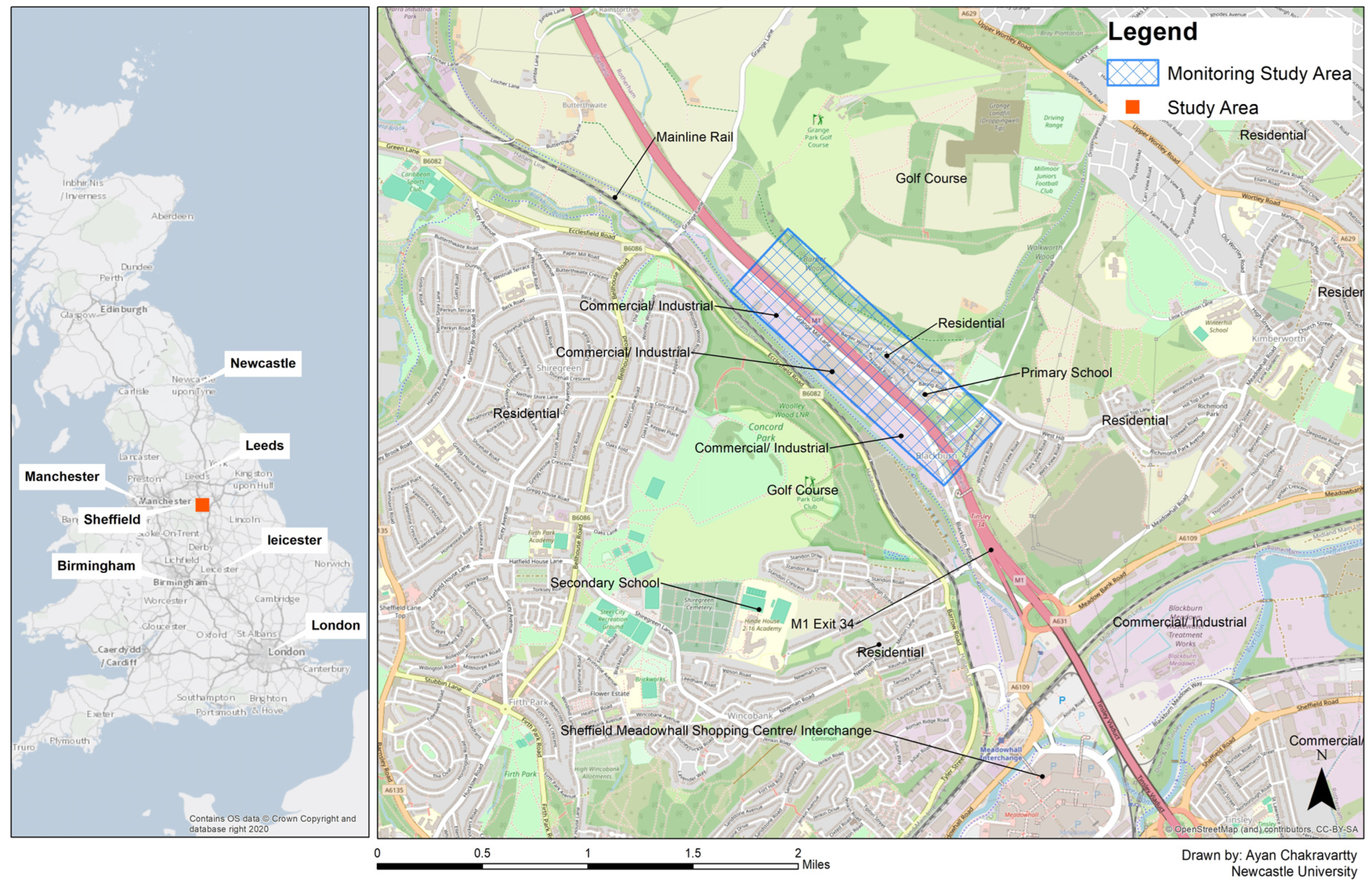
The M1 motorway, a critical transport corridor in the UK serves as ideal case studies for assessing the impacts on noise of these SMVSL interventions. For this research, a specific location in an AQMA on the motorway north–west of Junction 34, the intersection of the A6109 with Sheffield to the south–west and Rotherham to the north–east. The traffic volumes are high on eight lanes, with a significant proportion of HGV. The motorway traverses mixed land use, with sensitive receptors including schools and residential properties in close proximity (see Figure 1). Historically, the area has presented significant environmental challenges, including poor air quality and high noise levels.

Worthy of note is that the sensors were installed in mid-March 2020; so, all of the data were collected remotely during the COVID-19 lockdown period from April to September. Also, this period of monitoring was curtailed because, due to the COVID-19 lockdown rules, the e-Mote could not be serviced (pollution sensor replacement after 6 months), and the backup battery was repleted. However, given the fine resolution of the data, statistical significance of the results was achieved. Also, in the event, the atypical traffic flow characteristics that resulted from the COVID-19 lockdown rules on travel proved invaluable for this research. This was because the restrictions significantly altered traffic patterns, enabling a clearer separation of the impacts of heavy goods vehicles (HGVs) and other vehicles on noise pollution. With non-essential travel halted, the dominance of HGV traffic during this monitoring period provided unique insights into their disproportionate contribution to noise levels. This natural experiment, afforded by the pandemic, allowed this research to evaluate the role of SMVSL in mitigating noise impacts under different traffic scenarios, yielding findings with broader implications for traffic management and environmental policy on other road types.

3. Data Collection, Processing, and Analysis Methods

This study builds on previous research which explored the interaction of traffic dynamics, meteorological conditions, and noise pollution in urban environments [15]. Acoustic measurements were conducted using e-Mote sensors installed at a roadside location. The sensors recorded noise levels in real-time at one-minute intervals and subsequently synchronised with independent measurements of traffic and meteorological data. The noise data were processed and analysed to evaluate variations under different traffic conditions.

Bell and Galatioto highlighted the value of low-cost monitoring technologies for high-resolution environmental noise assessments [15], while Marouf et al. established correction algorithms to enhance the accuracy of measurements using inexpensive microphones for trend analysis [21,22]. These algorithms are incorporated into the low-cost e-Mote technology by the manufacturer Envirowatch, resulting in good quality noise data and providing data to an accuracy of better than 3 dBA. The e-Mote also provides measurement of air quality, including nitrogen dioxide, nitric oxide, and carbon monoxide, as well as temperature and humidity, the analysis of which forms the basis of a separate publication that is in preparation.

Previous research in urban areas [15,21,22] has demonstrated that the e-Motes track the variation of noise influenced by traffic dynamics; therefore, a low-cost sensor system was deployed at the side of the M1 in the vicinity of a set of MIDAS, Motorway Incident Detection and Automatic Signalling, loops, which provided traffic flow and speed data as one-minute averages separately for each of eight lanes (four in each direction), see Figure 2. Given that working on motorways is highly dangerous, bespoke training and certification are required. Therefore, the Envirowatch low-cost e-Mote sensor was installed by Amey Consult Ltd., and data were made available with the kind permission of the National Highways. The location provided unobstructed measurements of noise levels emanating from the traffic streams, which included four lanes of traffic in each direction. Air quality monitoring is not only influenced by the local air flows affecting dispersion but also by the chemistry of the interactions in the atmosphere. On the other hand, environmental roadside noise levels predominantly depend on the degree of attenuation, which is a function of road surface and distance and, therefore, is more directly influenced by traffic flow characteristics and meteorological conditions.

The data needed for the research presented in this paper are from three primary datasets: environmental noise levels, traffic characteristics, and meteorological conditions. Measurements were captured continuously between April 2020 and September 2020, encompassing the periods of SMVSL operation (from 07:00 h to 19:00 h on weekdays) with non-operation outside these times on weekdays and throughout the weekends. Noise levels LAeq at one-minute intervals and LAmax were recorded remotely by Envirowatch Ltd. (South Shields, UK) Traffic data at one-minute averages, including flow, speed, and fleet composition, were obtained from the Motorway Incident Detection and Automatic Signalling (MIDAS) loop detectors [23] installed along all UK motorways. MIDAS loop detectors provide high-resolution data for all eight lanes at the case study site. Meteorological conditions data, including wind speed, direction, temperature, and humidity, were sourced from the nearest weather station, at a 30 min resolution, which is located approximately 15 miles east of the study area, as shown in Figure 2. Wind speed and direction data from the UK National Meteorological Office weather station is ratified and available at 30 min intervals. The Met Office has a weather station network across the whole of the UK, with more than 200 automatic stations. The consistency of measurements in the records across weather stations is ensured by meeting strict criteria. These are aligned with meteorological organisations across the world and include specific standards on the levels of grass cover within the observation area. In addition, they require sufficient clear space for the weather station to be free from the influence of non-meteorological factors on the readings. In this way, the measurements are representative of an area some 40 miles around the station. The wind speed, direction, temperature, and humidity data captured from the Met Office were analysed alongside noise data to assess meteorological influences on noise propagation.

The data from eight traffic lanes, e-Mote, and Met stations were collated, synchronised, and processed for input to the analysis software packages. Noise levels from the e-Mote, traffic data from MIDAS loops, and meteorological data from the nearest weather station were first synchronised to the Greenwich Mean Time, GMT standard clock time, to ensure consistency across datasets. Outliers and missing values in the dataset were identified and addressed using interpolation for periods of ≤3 min or labelled otherwise. The analysis was based on mixed methods and included descriptive and hierarchical cluster analysis. The software packages used were the R and associated libraries described by [24], ensuring the integrity and robustness of the analysis.

The analysis focuses on identifying distinct noise regimes under varying traffic and meteorological conditions, with an emphasis on understanding the role of heavy goods vehicles (HGVs) in creating disproportionate noise impacts.

The initial phase of the analysis focused on investigating trends and the variability in noise levels influenced by traffic and meteorological conditions. Noise metrics, including equivalent continuous sound levels (LAeq) and maximum sound levels (LAmax), were assessed for temporal patterns and the effect of SMVSL operations. Temporal profiles were generated using one-minute resolution noise data collected from the e-Mote sensors, facilitating a granular analysis of diurnal and weekly patterns.

Descriptive statistics, including means, medians, standard deviations, and percentiles, were calculated as noise metrics to quantify variability across different operational conditions. Meteorological influences were explored using wind roses, and pollution roses were generated to visualise the directional dependency of noise levels on wind speed and direction. Additionally, time-series plots revealed dynamic changes during peak and off-peak hours, highlighting how SMVSL systems modulated noise levels.

Hierarchical Cluster Analysis (HCA) was conducted to classify the noise data into distinct categories based on traffic flow, vehicle composition, and meteorological conditions. The clustering process followed the methodology outlined by Kassambara [25]. This included an initial assessment of the clustering tendency using parameters such as the Hopkins statistic, a measure used to assess the tendency of a dataset to form clusters, and Visual Assessment of cluster Tendency (VAT), which is a heatmap image displaying pairwise distances between data points to highlight whether a dataset has potential to form distinct clusters. These methods were used initially to explore whether the dataset exhibited meaningful patterns suitable for clustering.

The optimal number of clusters was determined by employing several validation techniques, including the Elbow method, Silhouette analysis, and Gap statistics. These approaches quantified the quality of clustering results by assessing intra-cluster cohesion and inter-cluster separation. Based on these assessments, the data were segmented into clusters that reflected distinct noise profiles associated with different traffic and environmental conditions.

Agglomerative clustering with Ward’s linkage was used to group observations into clusters by minimising within-cluster variance. This method ensured that the clusters were homogenous and interpretable in terms of noise characteristics, traffic composition, and meteorological influences. For each cluster, descriptive statistics were calculated to identify the unique features of noise levels, such as the dominance of HGVs or the influence of specific meteorological conditions.

Visualisations, including dendrograms and box plots, were generated to summarise the clustering results and highlight the differences in noise profiles across clusters. For instance, certain clusters exhibited higher variability in LAmax values, often associated with higher proportions of HGVs, while others may show a more stable noise profile under smoother traffic flows during SMVSL operation.

This clustering approach not only provides a nuanced understanding of the noise dynamics on the M1 motorway but also demonstrates the value of high-resolution monitoring data for assessing the environmental impact of traffic management systems.

The results are presented in the next section.

4. Results

This section presents the findings from the analysis of the high-resolution monitoring of environmental noise along the M1 motorway, focusing on the impact of SMVSL systems. First, the results of the exploratory statistical analysis of traffic, speed, and noise are presented before all the data are brought together in the HCA.

4.1. Trend in Environmental Noise Level in the Study Area

Due to the lack of long-term measured noise data, traffic flow, speed, and proportion of heavy goods vehicle data from the Department for Transport (DfT) were used to estimate noise levels using the Calculation of Road Traffic Noise (CRTN) methodology [26]. This approach offers an indicative assessment of the potential year-on-year changes in noise levels and offers insights into trends in environmental noise levels within the study area from 2000 to 2022.

The annual average hourly traffic (AAHT) data show that 2000 (excluding 2020, which is atypical due to COVID-19 restrictions) had the lowest, whilst 2022 recorded the highest traffic levels, see

Table 1. Estimated CRTN noise levels at the E-MOTE site (2000–2022).

Year	AAHT	Traffic Volume Change (%)	HGV (%)	L10 (60 mph)	L10 (70 mph)	Noise Difference (dBA)
2000	4082	Base year	13%	80	84	4
2020	3628	−11%	11%	79	83	4
2022	4840	19%	10%	81	84	3
Avg	4506	-	11%	81	84	3

. The proportion of HGVs fluctuated between 9% and 13% over the period. CRTN-based calculations estimated that, at 60 mph, the average L₁₀ noise level was 81 dBA, whereas, at 70 mph, it was 84 dBA, corresponding to a 3 dBA increase. This 3 dBA change is significant, as it doubles the potential impact on human hearing and consequential health, highlighting the importance of managing vehicle speeds to mitigate noise pollution.

The CRTN results in Table 1 highlight that noise levels in 2000 compared to 2022 have remained relatively consistent, with the main fluctuations attributed to changes in traffic volume and HGV proportions. While the COVID-19 lockdown in 2020 led to a temporary reduction in traffic volumes, the associated reduction in noise levels was marginal and undetectable by the human ear at 1 dBA due to the continued operation of HGVs, which are demonstrated to be a dominant source of road traffic noise.

The estimated L10 levels reflect variations in traffic flow, speeds, and prevalence of congestion, with L₁₀ representing the noise level exceeded for 10% of the measurement period. The average 3 dBA difference between 60 mph and 70 mph underlines the critical role of speed in noise generation. Lower speeds not only reduce average noise levels but also lessen the long-term hearing health impacts, as per the IOSH guidelines [27]. Based on established dose–response relationships, an L10 noise level of 81 dBA at 60 mph corresponds to approximately 30% of people experiencing high annoyance. When the speed increases to 70 mph, raising the L₁₀ to 84 dBA, the proportion of people experiencing high annoyance rises to 36%, representing an increase of 6 percentage points in high annoyance. This highlights the significant impact of speed on noise-related disturbances, reinforcing the importance of speed management in mitigating noise pollution and its associated health risks.

Focussing on the study period, MIDAS data for 2019 were compared with the same period (from April to September) in 2020. The analysis revealed that noise levels at the monitoring location during the study period were not statistically significantly different from 2019 levels, despite much lower levels of car traffic and changes in traffic flow patterns due to the COVID-19 lockdown. This suggests that HGVs, which continued operating during lockdown periods, are the dominant source of noise in traffic streams. Reduced traffic volumes, particularly for passenger vehicles, did not significantly alter noise levels for all measures.

This CRTN analysis underscores the importance of speed management and traffic flow regulation, particularly on motorways, where a high proportion of HGV traffic exacerbates noise pollution. These estimates align with the broader policy objectives of the government, such as those outlined in the Noise Policy Statement for England (NPSE) [28], which aims to mitigate the adverse impacts of environmental noise on public health and residential amenities. However, these guidelines fail to reflect the variations in noise within hours at different average traffic levels, which change throughout the day. Variation of noise has been demonstrated to be more irritating than continuous noise levels at a lower average level [29].

Therefore, the data in this study were collated and synchronised at a resolution of one minute to better understand the link between traffic conditions and noise levels and, thus, to quantify the benefits of SMVSL on reducing the variation in noise, not just the levels. The next section presents an analysis of e-Mote data with Exploratory Statistical Analysis.

4.2. Traffic Flow and Speed Characteristics

The impact of SMVSL was evaluated by comparing the distributions of noise for weekdays from 07:00 h to 19:00 h when VSL was switched on, SMVSL-ON, with conditions, from 19:00 h to 07:00 h on weekdays, and for 24 h over the weekends when VSL was switched off, SMVSL-OFF. The summary statistics are presented in

Table 2. Summary statistics for noise, flow, and speed with SMVSL on and off.

Metric	Weekdays SMVSL On	Weekdays SMVSL Off	Weekends No SMVSL
Mean Noise (dBA)	73.93	68.63	70.11
Median Noise (dBA)	76.00	70.00	72.00
Noise Standard Deviation	6.76	6.18	7.31
Noise MAD	4.70	4.89	5.82

. Given that the noise distributions were of different shapes, the arithmetic mean, median, standard deviation, and median absolute difference (MAD) were derived to enhance the interpretation.

The mean noise level during weekdays when SMVSL was operational was 74 dBA, whereas it was 69 dBA when SMVSL was off overnight and 70 dBA during weekends when SMVSL was not operational. The median values followed a similar pattern, being different by 1 dBA or 2 dBA. This difference is within the sensitivity of the human ear to notice a difference and the measurement error of the e-Mote. The standard deviation and median absolute deviation indicate that noise variability was lower during SMVSL operation compared to other periods. The flow and speed characteristics showed that the mean flow was 24 vpm when SMVSL was in operation and 18 vpm when SMVSL was switched off, while the mean speed was reduced from 92 kph to 80 kph when SMVSL was active. Whilst these statistics reveal the impact holistically across the six-month period, the interaction of the speed and flow on noise levels in each minute is not revealed.

The sensor data provided further insights into noise parameters LAeq, LA10, LA90, and LAmax during the SMVSL-ON and SMVSL-OFF periods, as summarised in

Table 3. Summary of E-MOTE observed noise metrics during SMVSL-ON (daytime) and SMVSL-OFF (nighttime) periods.

Noise Descriptor	SMVSL-ON (dBA)	SMVSL-OFF (dBA)	Difference (dBA)
LAeq	79	74	5
LA10	80	78	2
LA90	78	68	10
LAmax	81	80	1

.

Daytime noise levels during SMVSL operation (SMVSL-ON) were lower and less variable compared to nighttime conditions when SMVSL was inactive (SMVSL-OFF). For example, the overall noise level (LAeq) was 79 dBA during SMVSL-ON and 74 dBA during SMVSL-OFF. The background noise level (LA90) showed an even greater difference, dropping by 10 dBA during nighttime conditions. The small 2 dBA difference in LA10 between SMVSL-ON and SMVSL-OFF highlights the consistent dominance of M1 motorway traffic, particularly HGVs, as the primary noise source in the study area. The steady HGV flows throughout the day likely contributed to elevated noise levels even during periods of reduced passenger vehicle traffic during COVID.

Figure 3 illustrates the one-minute noise levels (dBA) recorded by the e-Mote sensor as a function of the one-minute average speeds (kph), and the traffic flow (vpm) averaged over the eight lanes. The graph clearly shows how the noise levels are lower when the flows are low, and speeds vary from 30 kph to 190 kph in May, for example. The highest speeds occur when there is a lack of enforcement, creating peaks in noise, and, when the traffic is congested and stationary, the noise falls towards background levels. Congestion is coupled with unstable flow associated with acceleration and deceleration, which contributes to the variability in noise. As traffic flows increase, the speeds become less variable (due to smoothing of flow as drivers are unable to overtake and reach their desired speeds) and consequentially the noise levels increase, but the variability reduces. In August, however, there were periods of moderate and high flow levels that coincided with much lower noise levels. This is consistent with roadworks, which command a mandatory speed limit of 50 mph (80 kph) for all flow levels, which increases capacity and flows increase at the lower advisory speed. However, the increase in flow offsets, to a greater or lesser extent, the reduction in noise achieved by the lower advisory speed. The significant drop in noise levels is also consistent with the roadworks displacing traffic onto lanes further away from the monitored kerbside, reducing noise due to the attenuation over a longer distance. Against this interpretation, there are periods in the data when the SMVSL is operating and not operating. In order to gain further understanding, the data were disaggregated according to the SMVSL-ON/-OFF and analysed further. The analysis also indicates that the maximum speeds observed in the dataset were correlated with noise peaks, highlighting the importance of speed management in traffic noise mitigation.

Figure 3 illustrates the relationship between traffic speed, flow, and noise levels, demonstrating that reductions in traffic volume do not always correspond to lower noise levels. The increase in vehicle speed can offset the benefits of lower traffic density, leading to sustained or increased noise levels in the range of traffic conditions measured.

Figure 4 presents the noise level distributions under different traffic conditions. Figure 4a shows the noise level distribution for weekdays when SMVSL was operational compared to when it was switched off overnight and at weekends. Noise variability was much less under SMVSL operation, as the distribution, whilst shifted to the higher noise level, has much less spread compared to when SMVSL was switched off, with a wider flatter distribution, indicating greater fluctuations at a lower speed level. Figure 4b compares weekday SMVSL-ON noise levels to weekend noise levels, which exhibit similar trends. Weekend noise levels exhibited a wider range, showing increased variability and reaching higher levels of noise. This is consistent with the higher proportion of car traffic reaching higher speeds and, therefore, higher noise levels. Worthy of note is the lowest noise levels are consistent with traffic travelling at a lower speed during roadworks, which clearly spanned both weekdays and weekends.

Whilst this exploratory analysis provides a descriptive understanding of noise levels and variations influenced by changing traffic characteristics and speed control measures, they do not fully account for the combined effects of meteorological conditions and traffic dynamics on the noise at the measured minute/hour. However, to explore further the credibility of the e-Mote data, the next section compares the CRTN predictions for specific hours and days to further contextualise the findings before transitioning to an advanced statistical clustering approach that identifies distinct noise patterns under varying conditions in Section 4.4.

4.3. eMote Noise Data Analysis

The situation of COVID-19 prevented the co-location of a precision sound level meter for calibration; therefore, the observed noise levels were compared with CRTN-based estimates calculated from traffic data inputs, including total hourly flow, HGV percentages, road surface type, gradient, and speed, as shown in

Table 4. Comparison of CRTN predicted noise levels and E-MOTE observed noise levels during peak and off-peak periods on 8 September 2020.

Time Period	Traffic Flow (veh/h)	HGV (%)	Speed (mph)	CRTN L10 (dBA)	e-Mote L10 (dBA)	Difference (dBA)
07:00–08:00	2475	31%	57	85	80	5
19:00–20:00	1157	24%	66	82	79	3

. On 8 September 2020, during the morning peak (07:00–08:00), CRTN predicted an L₁₀ noise level of 85 dBA, whereas the E-MOTE data recorded 80 dBA, showing a 5 dBA difference. Similarly, during the evening period (19:00–20:00), CRTN predicted 82 dBA, while the E-MOTE observed 79 dBA, reflecting a 3 dBA difference. Whilst the latter is at the limit of the accuracy of the e-Mote (which was found to be 2.2 dBA [21]), the former was statistically significantly different. These differences highlight the role of site-specific conditions and sensor characteristics in noise monitoring. The e-Mote sensor accuracy of 2.2 dBA is within the acceptable limits defined in BS 4142:2014 and ISO 1996-1:2016 for environmental noise assessment.

The observed discrepancies between CRTN predictions and e-Mote measurements in Table 4 can be attributed to several factors. The e-Mote sensor, mounted at a height of approximately 2.5 m, was positioned at a height similar to the roadside barrier, potentially leading to reduced measured noise levels due to edge-of-barrier diffraction. In contrast, CRTN calculations assume a receiver height of 1.5 m, one meter below the e-Mote location. Furthermore, the e-Mote system, designed as a low-cost monitoring tool, has a 1 dBA resolution, 2.2 dBA accuracy, and sensitivity over the range of from 53 dBA to 93 dBA, compared to the broader sensitivity range of Class 1 reference noise monitors. While the CRTN methodology assumes idealised conditions, the e-Mote system has been demonstrated to respond well to changes in noise level and specifically captures real-world variations [21,22], including speed–flow interactions, with different fleet compositions and meteorological influences. Additionally, road surface and gradient assumptions, such as the bitumen surface type and 3% gradient used in CRTN calculations, may not fully reflect the variations in texture and slope that affect noise propagation. Despite these differences, 94% of the hourly e-Mote measurements agreed with CRTN predictions across the data-capture period.

The descriptive analysis underscores the value of SMVSL systems in reducing noise variability and stabilising noise levels, which provides acoustic benefits for nearby communities. However, the dominance of HGVs in overall noise emissions points to the need for targeted noise management strategies, such as promoting quieter technologies or implementing access restrictions during sensitive hours. While the e-Mote system offers a practical and scalable solution for noise monitoring, these findings also emphasise the importance of accounting for site-specific factors and sensor limitations in future studies to enhance the accuracy and applicability of noise assessments.

Whilst the descriptive statistics have shown considerable variation due to the interplay between speed, flow, % HGV, and the distance of the traffic from the e-Mote, the influence of meteorological conditions has not been considered, nor have specific patterns in all four variables with and without SMVSL been explored. Therefore, the next step in this research was to consider a more advanced statistical analysis. HCA was chosen as being the most suitable, however, due to the limitation of the computational power in the available computer, the dataset (traffic 8 × 3 (speed, flow, composition) + wind speed + direction and noise giving 27 variables every minute × 60 min × 24 h × 120 number of days) of 4,665,600 one minute recorded data was averaged to an hour for all variables, the results of which are presented in the following section.

4.4. Application of Cluster Analysis on Environmental Noise

The application of cluster analysis to the e-Mote noise data was used to identify any patterns within the data that influence the noise levels. Cluster analysis groups data based on the shared characteristics of the variables that govern specific noise environments. This section outlines the results of the clustering process, as outlined in Section 2, and demonstrates its appropriateness in analysing noise data.

4.4.1. Clustering Tendency Assessment

The clustering tendency of the dataset was assessed using the Hopkins statistic and Visual Assessment of Tendency (VAT). The Hopkins statistic was calculated using the ‘clustertend’ package in R [30], where the null hypothesis (H₀) assumes a uniformly distributed dataset with no meaningful clusters, and the alternative hypothesis (H₁) assumes the dataset contains meaningful clusters. The Hopkins statistic for the research dataset was 0.19, significantly below the threshold of 0.5 [25], indicating high cluster ability, whereas the random dataset returned a value of 0.53. These results, as shown in

Table 5. Assessment of clustering tendency results.

Dataset	Criteria	Hopkins Statistic
Research data	<0.5	0.19
Random dataset	<0.5	0.53

, demonstrate that the null hypothesis can be rejected, confirming the presence of meaningful clusters in the noise data.

Further, the VAT analysis employed Pearson distance measurements to construct a dissimilarity matrix. The VAT output revealed dark square blocks along the diagonal of the matrix, as shown on the left of Figure 5, indicating clusters of similar noise characteristics in the research dataset, whereas no such structure was observed in the random dataset, as shown on the right of Figure 5. These visual outputs confirm the clustering tendency of the research data and validate their suitability for further clustering analysis.

Having established that the data have a tendency to cluster, the next step was to define the optimal number.

4.4.2. Determining the Optimal Number of Clusters

The optimal number of clusters was identified using three methods: the elbow, silhouette, and gap statistics (see Figure 6). The elbow method suggested 4–6 clusters, silhouette analysis suggested 2–6 clusters, and gap statistics identified 3–6 clusters. To resolve these differences, the ‘NbClust’ library [25] in R was used to apply 23 additional indices. The majority rule from these indices identified four clusters as the most suitable choice.

4.4.3. Selection of Clustering Algorithm

The hierarchical clustering method was chosen for its robustness and suitability for the dataset, as validated by the ‘clValid’ library in R [25]. Hierarchical clustering was deemed more appropriate than k-means due to its lower sensitivity to outliers and its ability to handle the inherent variability in the noise data. The agglomerative approach was used to construct a dendrogram, which displayed the hierarchical relationships between data points and grouped them into four clusters.

In summary, the HCA results provided meaningful groupings of the noise data into four clusters, with each cluster reflecting unique characteristics of a combination of traffic flow, HGV proportions, and meteorological conditions that influenced specific noise environments. Clusters with high HGV proportions exhibited higher noise levels and variability, while clusters dominated by other vehicles, such as cars and vans, showed less variable noise profiles. The hierarchical tree plot (see dendrogram Figure 7) highlighted these distinctions, with fusion heights indicating the similarity or dissimilarity of data points within each cluster. The clusters were validated using internal measures, such as the silhouette coefficient and the Dunn index, to assess their quality and stability. These measures confirmed that the four identified clusters provided meaningful distinctions in noise characteristics/environments and were reliable for further analysis. The next section employs descriptive statistics to explore in more detail how the traffic and meteorological conditions influence the characteristics of the statistically significant differences in the four noise environments identified and establish the role of the SMVSL. In the following section, descriptive analyses have been carried out to allow a more in-depth understanding of the characteristics of the traffic and meteorological conditions that are influencing the noise levels.

4.4.4. Characteristics of the Clusters

The four clusters that emerged from the HCA were identified initially as C1, C2, C3, and C4, each representing unique noise environments.

Table 6. Descriptive statistics for noise level parameters across the four clusters (C1, C2, C3, and C4).

Statistic	C1	C2	C3	C4
Mean Noise (dBA)	69	75	57	71
Median Noise (dBA)	69	75	57	78
Mode Noise (dBA)	69	76	57	79
Standard Deviation	3	3	3	10
Kurtosis	0	0.4	29	−2
Skewness	0.2	−1	6	−0.4
Minimum Noise (dBA)	62	64	57	57
Maximum Noise (dBA)	77	81	74	80
Cluster membership	607	690	196	231

summarises the descriptive statistics derived from arithmetic averages of the hourly noise data for each of the data members of the four clusters in turn. The membership number of each cluster is provided for completeness. The clusters differ in terms of noise levels, traffic flow, and speed, reflecting the interplay between these variables in shaping environmental noise specific to each cluster. The characteristics of the noise are investigated before the role of the influencing variables, speed, traffic, and meteorological conditions, are explored.

Cluster C3 exhibited the lowest arithmetic average hourly noise levels, while Cluster C2 had the highest. Interestingly, Cluster C3 demonstrated high kurtosis and skewness, indicating a more peaked and yet heavy-tailed distribution, whereas C1 and C4 exhibited wider spread distributions with lighter tails.

Clusters C1 and C4 demonstrated more uniform traffic conditions, with lower variability in noise levels. The lowest noise levels in C3 were associated with lower traffic flow and speed, possibly due to the reduced non-HGV traffic during April, as confirmed by cluster-specific temporal analysis. The e-Mote sensors, despite limitations in their sensitivity range (53–93 dBA), successfully captured these nuanced noise profiles.

The shape of the noise distribution was tested for log-normality using the Q-Q and P-P plots. Whilst both Cluster C1 and C2 were found to follow a log-normal distribution, as determined using the Cullen and Frey [31] methodology, Cluster C1 had a short positive tail and C2 a negative tail, as confirmed by the skewness in Table 6 and Figure 8 and Figure 9. Clusters C3 and C4, on the other hand (see Figure 10), show distinctive patterns. In the case of C3’s distribution, except for 1.53% of the events at a level of 73 dBA and 1.02% at 74 dBA, all data are at 57 dBA. Noise levels below 53 dBA were not differentiated due to the limitation of the e-Mote sensor’s measurement range (see Envirowatch technical specifications in Section 2); therefore, this suggests that a background level L90 of 57 dBA prevailed throughout the monitoring period. Cluster C4 displays a bi-modal distribution, indicating two distinct noise level groupings in the lower mode, which are associated with the overnight and during roadwork periods.

How the noise parameters (LAeq, LA10, LA90, and LAmax) for each cluster relate to traffic speed and flow and meteorological conditions are presented in

Table 7. E-MOTE observed noise parameters (L_Aeq, L_A10, L_A90, and L_Amax) for each cluster (C1, C2, C3, and C4).

Noise Parameter	C1	C2	C3	C4
LAeq (dBA)	69	75	55	72
LA10 (dBA)	73	78	57	79
LA90 (dBA)	65	71	57	57
LAmax (dBA)	77	81	74	80
Average Speed (kph)	98	104	101	103
Average Wind Speed (m/s)	7	11	11	12
Average Wind Direction (Degrees)	199 (SSW)	187 (S)	160 (SSE)	217 (SW)

. Clusters C1 and C2 have higher values of LA90, a measure of the background noise, compared to C4, C1, and C2, which have lower LA10 and significantly lower values of the difference between LA10 and LA90 (a measure of variation or irritation to noise). C1, C2, and C4 with LAeq of 69 dBA, 75 dBA, and 72 dBA reflect the differing shapes of the distributions of noise with C1 skewed to the lower and C2 to the higher noise levels and with C2 being bimodal. C3, on the other hand, exhibits significantly lower levels of all noise parameters, with LA10, LAeq, and LA90 all less than 57 dBA, reflecting a much quieter acoustic environment and representing the prevailing background level at this study site. Worthy of note, however, is that the background noise levels are interrupted by the higher levels of noise associated with HGVs, which affect the LAmax levels. Only 2% of the time is likely to be during nighttime, potentially disturbing sleep. This requires further research to understand whether traffic is related or not.

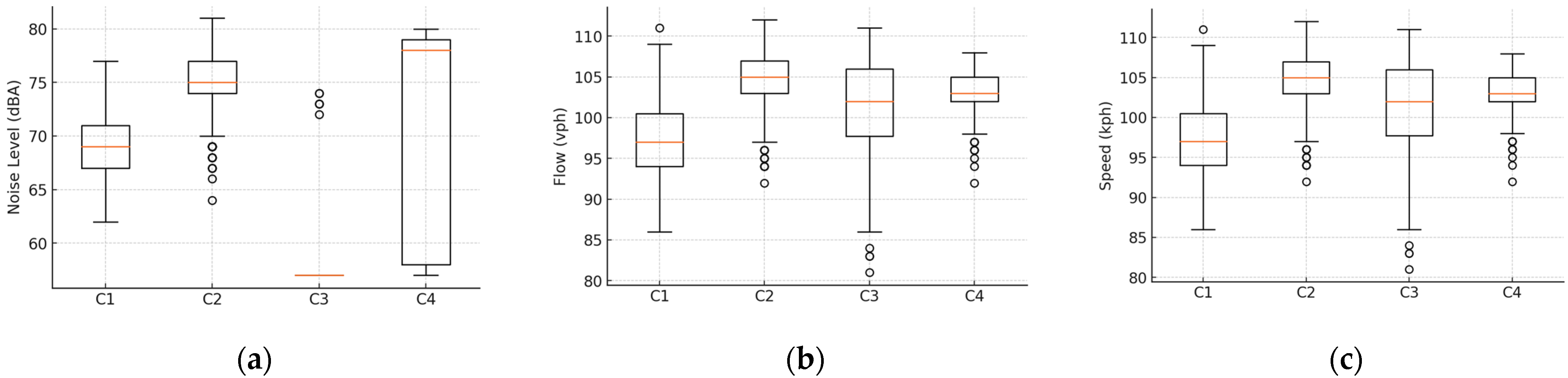
Cluster differences in relation to traffic and meteorological conditions are further explored with reference to Table 7 and Figure 11, where box-and-whisker plots summarise the quartiles and outliers for noise level, LAeq dBA, traffic flow, and speed for all four clusters. The plots show the central tendency, variability, and outliers of noise levels. Cluster C4 exhibited the highest flow level and smallest speed variation, resulting in the largest spread (interquartile range) in noise level. On the other hand, compared to C4, Cluster C2 displayed the highest but statistically similar speeds, and a marginally higher spread in traffic flow but at a statistically significantly lower flow level of 690 v/min. C2 has a statistically similar noise level to C4 but with a much smaller interquartile range. C3, on the other hand, exhibited the lowest noise levels at low traffic flow with a small amount, 2.6%, of noise events over 72 dBA and with the highest spread in speed, which was statistically similar to Cluster C2 and C4. Cluster C1 has a spread in noise level similar to C2 but at a statistically significant 6 dBA lower noise level and with the lowest speeds and traffic flows of all clusters. C2 and C3 exhibit outliers in noise but at low levels in C2 and at high levels in C3. C1 has outlier flows and speeds at high levels. C2, with a longer tail towards the high levels, has periods of low speeds, which may explain the outlier’s low noise levels. C3 is particularly interesting in the sense that it has a long tail without outlier flows but exhibits high noise outliers, yet outlier speeds are low. A similar pattern emerges in C4, with a long tail in traffic flow with outliers whilst outlier speeds are at low levels. Given that high speeds, high flows, and a high %HGV manifest themselves as drivers for high noise levels, there are other variables coming into play. The effect of weather will be explored next.

The relationship between wind conditions and noise levels within clusters was examined using polar plots, as shown in Figure 12. The diagram indicates the direction of the source noise relative to the receptor (centre of the plot) and the strength of the wind. Clusters C1 and C2 showed consistency in noise, over all wind directions, and speeds and were dominated by traffic noise from the M1 motorway. Cluster C3 displayed higher noise levels in the upper northeast quadrant when wind speeds were ~15 mph, suggesting contributions from non-M1 sources. In Cluster C4, higher noise levels were predominantly associated with M1 traffic. Quieter noise levels coincide mainly with strong south-westerly winds in C3 and south and south-easterly winds in C4. These polar plots provide a novel approach to examining the influence of wind direction and speed on noise propagation in traffic-dominated environments. However, the general distribution of wind direction, mainly from the southwest, for the data was similar across all clusters except Cluster C4, where the winds were fairly uniform from all directions. Worthy of note is that the noise received at the monitor is across eight lanes of traffic. Generally, the lanes with the highest traffic flows and highest percentage of heavy goods vehicles are the closest and furthest lanes away from the receptor. Traditionally, the source line of the noise is defined as the centre of the road. The use of a centre-line noise source assumption follows the Calculation of Road Traffic Noise (CRTN) 1988 methodology, which is one of the standard practices for UK motorways and other road source-based noise assessments. This study accounts for noise from both traffic directions using a balanced averaging approach. While lane-specific effects may be explored in future studies, the tested method aligns with established UK environmental noise policies and available traffic data.

In summary, the noise environment of C1 is dominated by both the lowest of flows and speeds and a moderate to high percentage of HGV; C2, with medium flows, high speeds with low variation, and outliers at low noise levels; C3, with all noise parameters, except LAmax at 57 dBA, represents the prevailing background level at moderate speeds; C4, on the other hand, has a significantly wider spread of noise level, with the highest and smoothest of flows and speeds (narrowest spread). On the other hand, the influence of meteorological conditions, whilst similar in all clusters, clearly demonstrated the motorway traffic as the significant local source of noise northeast of the monitoring location.

The descriptive statistics and visualisations reveal distinct noise characteristics within each cluster, driven predominantly by the variations in traffic flow and speed, with meteorological conditions having less influence. The findings demonstrate the effectiveness of cluster analysis in identifying meaningful patterns in environmental noise and influencing factors, providing potential for the guidance of noise mitigation strategies. Whilst this analysis reveals generic differences in the characteristics of each cluster, the next section takes up further discussion to explore the interrelationships between speed, flow, and noise to gain a deeper understanding and to establish the influence of the SMVSL.

5. Discussion

The previous section clearly identified patterns in the interplay between speed and flow as well as the percentage of HGV having a significant influence on noise levels. The LAeq noise level data for each cluster are now discussed further in the context of the dual impact of speed and flow to establish the influence of the SMVSL on noise levels. Figure 13, Figure 14, Figure 15 and Figure 16 present, respectively, for C1, C2, C3 and C4, the influence of speed and flow on noise levels (top left of the figures), heavy goods vehicle proportion (bottom left), day of the week (top right), and whether SMVSL is operating or not (bottom right). Please note that to discuss the features of a specific cluster in context, all other one-hour data are plotted in grey in the background of each graph.

Cluster C1, characterised by high noise levels, low traffic flow, and variable speeds, was dominated by moderate to high HGV volumes (Figure 13 bottom left), which demonstrates the clustering of data points at a low flow that are clearly separated from other clusters, emphasising the impact of HGVs on noise profiles.

These conditions were primarily observed overnight and on weekends (Figure 13 top right), when the SMVSL was switched off, and during off-peak hours with wind directions, particularly at higher speeds, predominantly blowing across the motorway towards the monitor. The dominance (weekdays, Figure 13 top right) of this cluster aligns with the periods of reduced car traffic and highlights the disproportionate contribution of HGVs to environmental noise under non-SMVSL conditions overnight.

Cluster C2, as shown in Figure 14, exhibited higher noise levels than C1, with increased traffic flow and occupancy but lower HGV proportions. The cluster was primarily associated with weekdays and dominated by peak and off-peak traffic under SMVSL operation. The findings suggest that, while SMVSL operation led to reduced speed variability at speeds around 60 mph (97 kph), higher vehicle flows resulted in a marginal increase in noise levels, consistent with the relationship between flow and noise having a smoothing effect on flows. The influence of HGVs was relatively lower than in C1, given that the higher speeds occurred mostly at weekends when the proportion of HGVs was lower. These results suggest that SMVSL systems effectively regulate higher speeds, enabling a greater flow of traffic due to smoothing whilst mitigating peak noise events generally caused by the braking and acceleration of unstable flow. However, the human ear perceives changes in noise levels of 3 dBA and above, suggesting that the observed 2 dBA difference in noise between C1 and C2 would be imperceptible to most individuals. Changes below 3 dBA are generally imperceptible to the human ear, while changes of 3 dBA and above are noticeable but not necessarily significant. Environmental noise assessments typically consider a 5 dBA change as the threshold for a significant impact, as per BS 8233:2014 [32] and ISO 1996-1:2016 [33]. On the other hand, smoothing of flows above about 10 veh/min (Figure 14 bottom right) emphasises the effect of SMVSL operation on noise by regulating speeds and reducing variability in the noise.

Cluster C3, with the smallest cluster number of observations (160), represents the quietest noise environment (LAeq 55 dBA), with low traffic flows at lower speeds (Figure 15 bottom left) during weekdays and higher traffic flows during weekends. The cluster was dominated by HGVs travelling overnight (top right) during SMVSL-OFF conditions during the week (bottom right), while weekend traffic was characterised by non-HGV traffic at higher speeds, consistent with the effects of lockdown periods.

Cluster C4 in Figure 16 shows (top left) that the highest total traffic flow coincides with the high noise level (LAeq up to 72 dBA), which is primarily associated with weekday traffic (top right) during SMVSL-ON conditions (bottom right). Note that the hours with reduced speeds observed in this cluster were consistent with mandatory speed limit operation at 50 mph, enabling maximum lane capacity during roadworks. The clustering of data around traffic speeds of 100 kph–105 kph (60 mph) is due to the SMVSL operation, which facilitates smoother traffic dynamics, albeit at the cost of higher noise levels due to the increase in flow whilst reducing unstable stop–start traffic.

Figure 16 shows how noise increases with speed, particularly at higher speeds, due to aerodynamic effects, but is also affected by traffic flow conditions. Therefore, this study supports the findings that noise does not relate to traffic flow and speed linearly but follows a logarithmic or power function, similar to aircraft noise models.

Worthy of note is that drivers in the UK are aware of the 10% rule, which is a guideline used by some police forces with regard to adhering to traffic speed limits before prosecution and, therefore, take the risk of driving above the speed limit. Figure 16 presents the distribution of C4, emphasising the role of SMVSL in managing high traffic flows while maintaining consistent noise profiles.

In summary, Cluster C4 showed the highest total traffic flow and a high noise level (LAeq up to 72 dBA), which were primarily associated with weekday traffic during SMVSL-ON conditions. The lower speeds across the range of flows mid-week with moderate and high % HGV during SMVSL operation at 50 mph are consistent with a period of roadworks, enabling a higher capacity of over 60 vehicles per minute to be achieved on four lanes instead of eight. Please note that the maximum capacity of a motorway lane is typically 1100–1900 vehicles per hour depending on the number of lanes, whether it is a rural or urban motorway, and what the proportion of heavy goods vehicles is. This analysis of traffic flow characteristics suggests that SMVSL operation facilitated smoother traffic dynamics, albeit at the cost of higher noise levels of about 2 dBA due to the increase in traffic volume facilitated by the operation of traffic at a speed of 60 mph instead of 70 mph. However, comparing the range of noise levels across the four clusters, it is clear that the variability in the noise is reduced with the operation of SMVSL.

An explanation for the reduced noise evident in Cluster C3 and Cluster C4 (Figure 15 and Figure 16) in relation to the meteorological conditions is that these data coincide mainly with the roadworks taking place in August and early September, during which the number of lanes was reduced to the four lanes furthest away from the e-Mote monitor. Despite an increased traffic flow (748 vehicles per hour) and relatively high average speeds (102.2 kph), the increased distance from the monitor contributed to increased noise attenuation, resulting in lower observed noise levels in these clusters. Furthermore, a detailed analysis confirms that 249 instances of noise levels below 60 dBA occurred consecutively in C3 and C4, supporting the claim that these conditions were sustained over a period rather than being isolated events and, therefore, associated with roadworks. These findings highlight how road infrastructure changes can impact noise levels and reinforce the role of traffic management and meteorological conditions in shaping environmental noise profiles.

The results underline the effectiveness of SMVSL systems in reducing noise variability and mitigating extreme noise events during peak traffic periods. Clusters C2 and C4, which predominantly represent SMVSL-ON conditions, demonstrate the benefits of regulated speed in minimising noise peaks while maintaining high traffic flow. However, the findings also highlight the disproportionate contribution of HGVs to overall noise levels, as seen in Clusters C1 and C3, suggesting a need for targeted measures to manage HGV-related noise.

It could also be noted that clusters C2 and C4 demonstrate that noise variability is potentially influenced by acceleration and deceleration cycles. The SMVSL system effectively reduces noise peaks by smoothing traffic flow, minimising abrupt changes in velocity, and mitigating acceleration-related noise spikes. Future research can investigate this in more detail.

Figure 13 and Figure 16 illustrate that the relationship between vehicle speed and noise follows a non-linear trend, consistent with established research that noise increases with velocity in a power-law manner. At higher speeds, aerodynamic noise becomes the dominant factor, particularly for light vehicles and electric vehicles, which rely less on engine noise at cruising speeds.

The use of polar plots (Figure 12) provides further insights into the influence of wind speed and direction on noise dispersion. Clusters C1 and C2 showed homogeneity in the patterns, indicating that noise levels were dominated by a single source, the M1 motorway. In contrast, C3 exhibited occasional higher noise levels, likely associated with non-M1 sources, given they occur for 2% of the data sample and only during northeasterly winds. The lower noise levels in C3 and C4 illustrate periods when the background noise levels prevail. The box plot (Figure 11) confirmed the differences in noise levels across clusters, with C4 showing the highest traffic flow and smallest speed variation, while C3 demonstrated the quietest conditions.

This study acknowledges meteorological influences, such as wind, temperature, and humidity. However, the analysis is limited to the available monitoring period (April–September). The road surface was Hot Rolled Asphalt, HRA, and research by Phillips and Morgan [34] showed that a reduction in air temperature of 25 °C for light vehicles increases the noise by 1.4 dBA and that there is no noticeable difference with change of humidity. This change in noise level is not perceived by the average human ear. Whilst providing an indication of the likely changes in noise levels, further work could repeat the data collection and analysis during the winter months to explore seasonal variations in noise propagation alongside a stretch of the motorway with SMVSL in operation. Worthy of note is that this estimated short-term change for different weather conditions is consistent with the long-term variation of 1 dBA observed by Klami et al. [35].

The analysis indicates that the high noise levels in Cluster C3 do not follow a regular daily pattern but instead appear sporadically. The average number of high noise events per day is 0.4, suggesting that these occurrences are relatively rare. Additionally, there are no consecutive periods where high noise levels persist over multiple days. This suggests that the elevated noise levels in C3 are likely associated with isolated events rather than a sustained trend over weeks or days. These findings indicate that temporary external factors associated with specific activities and weather influences can contribute to the high noise spikes in C3.

The proposed mixed method of analysis (HCA and descriptive) is transferrable to other datasets and case studies. All noise levels measured, even at significantly reduced travel during COVID-19, exceeded the 55 dBA recommended as an acceptable noise limit for human exposure. Therefore, sound barriers, displacement of newly built residential properties at a distance away from the motorway, or appropriate acoustic treatment of windows and walls are essential to protect those living in close proximity to motorways. A sound barrier is located at the study site, placing the nearby residential properties in an acoustic shadow.

6. Limitations and Future Research

The main limitation of the results of this research is the periods of missing data due to the fact that the e-Mote sensor system could not be maintained during COVID-19. Whilst the quality of the captured data was consistent with the e-Mote specifications, there was a loss of data when the backup batteries ran out of charge, and the e-Motes had to rely on the solar panels to charge the rechargeable batteries. COVID-19, on the other hand, provided an opportunity to demonstrate the range of impacts due specifically to the HGV, but the outputs are not representative of the traffic flows of today.

Therefore, future work should consider repeating the data capture, and a comparison with the results presented here will provide added value. The same study, with the cooperation of National Highways, could explore the extension of the SMVSL into the evening in order to smooth flows and operate at speeds that optimise HGV noise. Also, a simultaneous questionnaire survey of people’s perceptions of noise before and after the installation and operation of SMVSL on motorways would endorse the findings of the research presented in this manuscript. As vehicle fleets transition to electric powertrains and, for HGV and buses, to hydrogen, the interplay between speed, flow, and noise necessitates ongoing research and the appropriate modification of SMVSL operation.

The calibration of the noise measurement system was managed on behalf of National Highways by Amey, who installed the e-Mote sensors as part of the deployment process. The contract with Envirowatch, who supplied the e-Mote, involved the replacement of a backup battery when depleted and sensors every six months to ensure good-quality data. The eMote self-corrects the noise measurements within its data processing using the algorithms derived by Marouf et al. [21]. In addition, temperature and humidity within the sensor are measured to calibrate the air pollutants measured. However, the COVID-19 pandemic, imposed restrictions on fieldwork, sensor maintenance, and battery replacement, preventing additional on-site co-location validation with precision monitors. While the e-Mote sensors provided consistent and reliable data, future research could implement additional calibration steps to validate noise measurements under the same meteorological conditions on the same section of the road.

It should also be noted that this study does not differentiate between specific vehicle model types, but it is well established that aerodynamics, the tyre–road interaction, and vehicle design significantly impact noise emissions. Future work could incorporate vehicle model type classification to assess differences in aerodynamic noise contributions between traditional combustion vehicles and electric vehicles. As more electric vehicles replace traditional internal combustion engines, the dominant noise will be the road–tyre interface, particularly at higher speeds.

This study focuses on high-resolution noise variability, while long-term noise measurements at lower resolution provide complementary insights. Future research could integrate long-term monitoring alongside real-time noise fluctuation studies to better understand seasonal trends and the impact of traffic management and infrastructure investment.

Additionally, while the observed difference between L₁₀ and L_eq in this study remains within the expected range of 1.5–4.5 dB, long-term monitoring consistency could not be fully evaluated due to the lack of sensor maintenance during the pandemic. As the e-Mote sensors could not be regularly serviced or recalibrated, potential minor fluctuations in L₁₀ and L_eq differences due to external factors cannot be entirely ruled out. While this did not significantly affect this study’s conclusions, future research should ensure more frequent calibration and maintenance to further improve the long-term reliability of noise monitoring results.

While wind speeds exceeding 5 m/s can influence noise measurements, the eMote has an acoustic cap to shield the microphone and randomise the noise direction before entering the monitor. In addition, the monitoring site was partially shielded from strong winds by a noise barrier and adjacent residential buildings, minimising direct meteorological interference. Therefore, using the meteorological conditions data measured at a distance imposes limitations on this study. According to BS 4142:2014, meteorological effects should be considered in environmental noise assessments, but measurements are not automatically invalidated unless there is a substantial deviation affecting interpretation, which was not found to be the case in this study. Furthermore, noise monitoring was part of a broader research initiative aligned with simultaneous air quality monitoring, where meteorological factors play a critical role in pollutant dispersion. The correlation between traffic flow, meteorology, and environmental impacts will be presented in a subsequent publication. For the purpose of this study, the recorded noise data remain valid and provide crucial insights into real-world traffic noise dynamics under varying conditions. Future research could implement a monitor to capture temperature, humidity, and wind speed and direction data collocated with the eMote to further evaluate noise propagation under extreme meteorological conditions.

This study primarily considers the existing vehicle fleet composition during the monitoring period, where internal combustion engine (ICE) vehicles remain dominant. However, as the adoption of electric vehicles (EVs) increases, their influence on traffic noise emissions will evolve. At low speeds, EVs generate less propulsion noise due to the absence of an internal combustion engine, whereas, at higher speeds, noise is primarily governed by aerodynamic effects and tyre–road interactions, which affect all vehicle types. Future studies could incorporate detailed fleet composition analyses to assess the long-term noise implications of the shift from ICE to EVs, particularly in urban and motorway environments.

While this study primarily examines the impact of the implementation of the SMVSL on noise emissions, we acknowledge that road surface conditions, including asphalt wear and surface degradation, can influence noise propagation. Furthermore, the roadworks during September were associated with the replacement of motorway furniture, not the highway itself. The study location featured a highway-grade surface that was not undergoing resurfacing during the monitoring period, minimising road wear effects. Future studies could incorporate detailed assessments of road surface types, maintenance cycles, and surface texture variations to better understand their contribution to long-term noise emission trends.

The relationship between vehicle speed and noise levels is examined through hierarchical clustering, an unsupervised machine-learning approach that groups noise data into meaningful categories based on traffic and environmental conditions. The maximum speeds observed in the dataset contribute to the clustering framework, allowing for an interpretation of noise variation under different traffic regimes. However, due to computational limitations, clustering was conducted on hourly-averaged data, ensuring robust classification while managing the large dataset size. This averaging smooths out instantaneous speed fluctuations, meaning that extreme speed peaks are not explicitly isolated but are instead represented within broader traffic patterns. While this ensures robust pattern identification, it does not capture second-by-second fluctuations in extreme speed values. The clustering approach was adopted to meet this study’s objectives and provides a structured way to interpret noise variation across different traffic regimes, rather than focusing on individual maximum speed instances. Future research could explore higher-resolution clustering techniques or real-time processing methods to better capture short-term noise spikes due to extreme vehicle speeds. Notwithstanding, the descriptive analysis of the clusters is carried out at a resolution of 1 min, with HGV dominating the peak noise levels.

This study prioritises real-world noise monitoring to capture traffic noise variability under actual traffic conditions. Whilst software tools such as SoundPLAN and CadnA provide valuable capabilities for predicting noise levels under different traffic scenarios, they rely on propagation models and assumptions about vehicle distributions and speeds rather than direct individual vehicle-based measurements at one minute. Therefore, the advantage of real-world measurements is that they capture actual traffic dynamics, meteorological influences, and noise propagation patterns, which simulations often approximate using idealised conditions. However, predictive noise modelling tools, such as SoundPLAN and CadnaA, could complement future research by simulating noise propagation under different traffic scenarios. A hybrid approach could be explored, where empirical sensor data are integrated with traffic noise simulations to enhance model validation and predictive accuracy. This would allow researchers to compare measured vs. simulated noise levels, refine noise propagation models, and assess potential mitigation strategies for a range of different road environments.

7. Conclusions

This analysis set out to explore the role of SMVSL in supporting an improved acoustic environment and revealed four acoustic environments in the vicinity of the motorway, which are as follows:

C1: A high-noise environment with low traffic flow and variable speeds, predominantly influenced by heavy goods vehicles (HGVs). This cluster was largely associated with overnight and weekend traffic when the SMVSL was switched off, highlighting the disproportionate contribution of HGVs to environmental noise under non-SMVSL conditions.

C2: A moderate-noise environment with a higher traffic flow than C1 but lower HGV proportions. This cluster was associated primarily with weekday traffic during SMVSL operation, where regulated speeds and higher vehicle flows result in a more stable traffic pattern, reducing speed variability and mitigating peak noise events caused by acceleration and braking.

C3: The quietest acoustic environment, with the lowest traffic flow and lower speeds, was primarily influenced by overnight HGV movements during SMVSL-OFF conditions and higher-speed non-HGV traffic on weekends. Despite occasional high-noise events, these were isolated occurrences rather than sustained trends. The quieter conditions in C3 coincided with roadworks when lanes were shifted further from the noise monitor, resulting in noise attenuation.

C4: A high-traffic, high-noise environment primarily associated with weekday traffic under SMVSL-ON conditions. The reduced speeds at 50 mph during SMVSL operation facilitated smoother traffic dynamics while enabling maximum lane capacity, particularly during roadworks. However, the increased flow contributed to elevated noise levels, albeit with lower variability due to the stabilising effects of SMVSL.

Overall, the findings emphasise the critical role of SMVSL systems in managing traffic flow and speeds to reduce noise variability. Whilst the regulation of speed under SMVSL operation benefits residential communities by mitigating noise peaks, the dominance of HGVs in noise emissions suggests the need for further interventions, such as promoting quieter vehicle technologies and a mode shift of heavier freight onto rail, potentially considering freight traffic rescheduling away from the middle of the night or operating SMVSL at the optimum quiet speed for HGV. These insights provide a foundation for developing integrated approaches to mitigate the noise impacts of road transport and enhance urban living conditions.

The clustering approach provided a detailed understanding of the noise regimes, identifying patterns influenced by traffic dynamics, meteorological conditions, and SMVSL operations. Also, this research has demonstrated the value and importance of studying noise levels at a finer resolution along with simultaneously measuring traffic fleet composition, flows, speeds and meteorological conditions in order to gain a fundamental understanding of their complex interactions. Furthermore, this research demonstrated the need for finely resolved data to provide comprehensive insights into the role of SMVSL systems in managing environmental noise along a motorway.

The M1 section of the motorway northeast of Sheffield was chosen not only for its strategic importance within the UK’s road network but also because the impacts of the traffic on the environment experienced by communities are typical of those living near major motorways and trunk roads. However, the COVID-19 pandemic, whilst presenting an opportunity to enrich understanding, renders the magnitude of the impacts emerging from this analysis specific to this study. However, the methodological approach using a combination of descriptive statistics and HCA is directly transferrable to other sites along motorways and urban areas provided similar traffic data, available at a 1 min resolution, to other road types.

We conclude that investment in SMVSL systems effectively reduces noise variability by 6% by mitigating extreme noise events, particularly during peak traffic periods. This potentially reduces noise annoyance, with significant improvements in the health of exposed populations. However, by smoothing traffic flow and regulating speeds, SMVSL operations increase traffic volumes, which, in turn, increases LAeq noise by 2 dBA, a difference imperceptible to the human ear. Despite the demonstrated benefits of SMVSL systems in noise management, the results also highlight challenges, including the need for further interventions to enhance noise mitigation, such as promoting quieter vehicle technologies and optimising traffic flows overnight. Additionally, as vehicle fleets transition to electric powertrains and hydrogen, the interplay between noise, flow and speed is expected to be different, necessitating adaptive policies and ongoing research.

The detailed technical descriptions in this paper provide essential context for engineers and scientists to understand noise variability under different traffic conditions. In turn, this will inform decision-making regarding how SMVLS could be used to better manage noise variations overnight to avoid sleep disturbance on stretches of road where residential properties are located close to trunk roads as well as motorways. This foundational analysis will support future work focusing on advanced statistical modelling using AI and predictive analysis of traffic noise.