Influence of the Gain–Bandwidth of the Front-End Amplifier on the Performance of a QEPAS Sensor

Abstract

The quartz tuning fork used as an acoustic sensor in quartz-enhanced photo-acoustic spectroscopy gas detection systems is usually read out by means of a transimpedance preamplifier based on a low-noise operational amplifier closed in a feedback loop. The gain–bandwidth product of the operational amplifier used in the circuit is a key parameter which must be properly chosen to guarantee that the circuit works as expected. Here, we demonstrate that if the value of this parameter is not sufficiently large, the response of the preamplifier exhibits a peak at a frequency which does not coincide with the series resonant frequency of the quartz tuning fork. If this peak frequency is selected for modulating the laser bias current and is also used as the reference frequency of the lock-in amplifier, a penalty results in terms of signal-to-noise ratio at the output of the QEPAS sensor. This worsens the performance of the gas sensing system in terms of ultimate detection limits. We show that this happens when the front-end preamplifier of the quartz tuning fork is based on some amplifier models that are typically used for such application, both when the integration time of the lock-in amplifier filter is long, to boost noise rejection, and when it is short, in order to comply with a relevant measurement rate.

1. Introduction

The quartz-enhanced photo-acoustic spectroscopy (QEPAS) technique is a typical application in which a resonant piezoelectric sensor is used to detect acoustic waves, in this case generated by the interaction between a laser beam and a gas sample. In gas detection systems based on QEPAS, the resonance properties of a quartz tuning fork (QTF) are exploited to enhance the electric signal resulting from the interaction between a modulated laser source and the target gas [1,2,3,4]. As shown in the schematic diagram of Figure 1, the intensity of a laser source of suitable wavelength, chosen according to the absorption line of the molecules to be detected, is modulated at a given frequency f₀. Non-radiative, periodic relaxation processes of the gas molecules, excited by the modulated laser light, generate sound waves that are efficiently transformed into electric signals by means of the QTF, if the laser modulation frequency is tuned to the resonant frequency f_s of the crystal or one its sub-harmonics. A lock-in amplifier (LIA) is used to demodulate the signal generated by the QTF and produces a DC output voltage proportional to its amplitude, which, in turn, is proportional to the concentration of the target gas.

Since the QTF is an acoustic quadrupole resonator, the sound waves produced by sources external to the prongs tend to move them in the same direction, which does not result in an appreciable electric signal, since this kind of deformation of the prongs is not piezoelectrically effective. Only the sound waves generated between the prongs are able to excite a useful signal; thus, an excellent immunity to environmental acoustic noise is achieved [2].

Furthermore, the acoustic waves generated by the interaction between the laser light and the molecules to be detected are very weak, so, usually, an acoustic micro-resonator filled with the same gas is added to increase the effective acoustic interaction length between the sound waves and the QTF. The resonator is composed by two small tubes placed perpendicularly to the plane of the QTF and aligned to the space between the prongs at a suitable distance from them, as shown in Figure 2 [5].

In this arrangement, the QTF probes the acoustic waves generated by the interaction of the laser beam with the gas contained inside the tubes. Concerning the resonance properties of the QTF, its Q factor decreases due to the acoustic coupling between the tubes and the QTF itself, whereas its resonance is slightly shifted towards higher frequencies. A suitable choice of the length of the micro-resonator tubes, their diameter, the gap between the two tubes, and the position of the acoustic resonator along the prongs of the QTF allows an increase in the QEPAS sensitivity by a factor of more than 10 to be achieved [5].

The QEPAS technique has been proven to be very compact, sensitive and reliable, enabling sub-ppm and even sub-ppb minimum detection limits [6,7,8].

Since the Q factor of typical QTFs used in QEPAS sensors is very high, with an order of magnitude of several thousands [9], the frequency of the laser modulation signal and the lock-in reference frequency must be carefully selected in order to fully exploit the resonance properties of the QTF and maximize the signal-to-noise ratio (SNR) of the sensor.

Although voltage-mode front-end preamplifiers for the QTF have been proposed in the literature [10,11,12,13], the most common circuit configuration for interfacing the QTF is still the classic transimpedance preamplifier (TIA), schematically represented in Figure 3 [14,15,16,17].

If the loop gain of the circuit in Figure 3 is large enough, the inverting input terminal of the operational amplifier (OPAMP) can be considered a virtual ground. This makes the current signal I_QTF generated by the QTF independent of parasitic components, such as the input capacitance of the OPAMP C_IN. Furthermore, the current I_F that flows in the feedback resistor R_F is equal to I_QTF; thus, the output signal V_OUT depends only on the characteristics of the piezoelectric sensor and on the value of R_F:

$${\mathrm{V}}_{\mathrm{O}\mathrm{U}\mathrm{T}}=-{\mathrm{R}}_{\mathrm{F}}{\mathrm{I}}_{\mathrm{Q}\mathrm{T}\mathrm{F}}.$$

(1)

The response of the TIA exhibits a sharp peak at the series resonant frequency f_S of the QTF, which as a consequence is the most suitable operating frequency for the QEPAS sensor. The value of this frequency is usually identified using the same TIA by disconnecting from ground the QTF terminal, applying a sinusoidal voltage signal to this terminal, and scanning the frequency around the expected value of f_S, until the peak amplitude of V_OUT is reached [18].

As already pointed out, the ideal behavior of the circuit described above is strictly related to the presence of the virtual ground at the inverting input of the OPAMP, which, in turn, is effective only if the loop gain of the feedback loop is much larger than unity. Usually, in order to guarantee that this condition is fulfilled, it is deemed sufficient to use an OPAMP with a gain–bandwidth product (GBW) much higher than the operating frequency. For instance, in case of a classic QTF with f_S = 32.768 kHz, low-noise OPAMPs with a GBW of a few MHz have often been used [10,11,13,16]. In this work, we demonstrate that, due to the behavior of the QTF around its resonant frequency, much larger values of the GBW are needed to guarantee a good virtual ground for the TIA at these frequencies. In cases in which an amplifier with an insufficient bandwidth is used, some undesirable phenomena occur. First, the peak frequency of the circuit response f_peak is no more located at the intrinsic f_S of the QTF, but is shifted to lower frequencies; thus, the characterization procedure described above is no more able to provide the intrinsic resonance frequency of the piezoelectric sensor. Moreover, some contributions to the total output noise are strongly affected by the missing virtual ground and, as a consequence, the operating frequency at which the maximum SNR is obtained can be different from the frequency f_peak. Thus, in this case, the characterization procedure is no more able to provide the optimal value for the operating frequency of the QEPAS sensor. In any case, it will be shown that the SNR performance obtained is sub-optimal if compared to the case in which it is possible to achieve good performance if an OPAMP with the same noise characteristics but a much larger GBW is used.

2. Materials and Methods

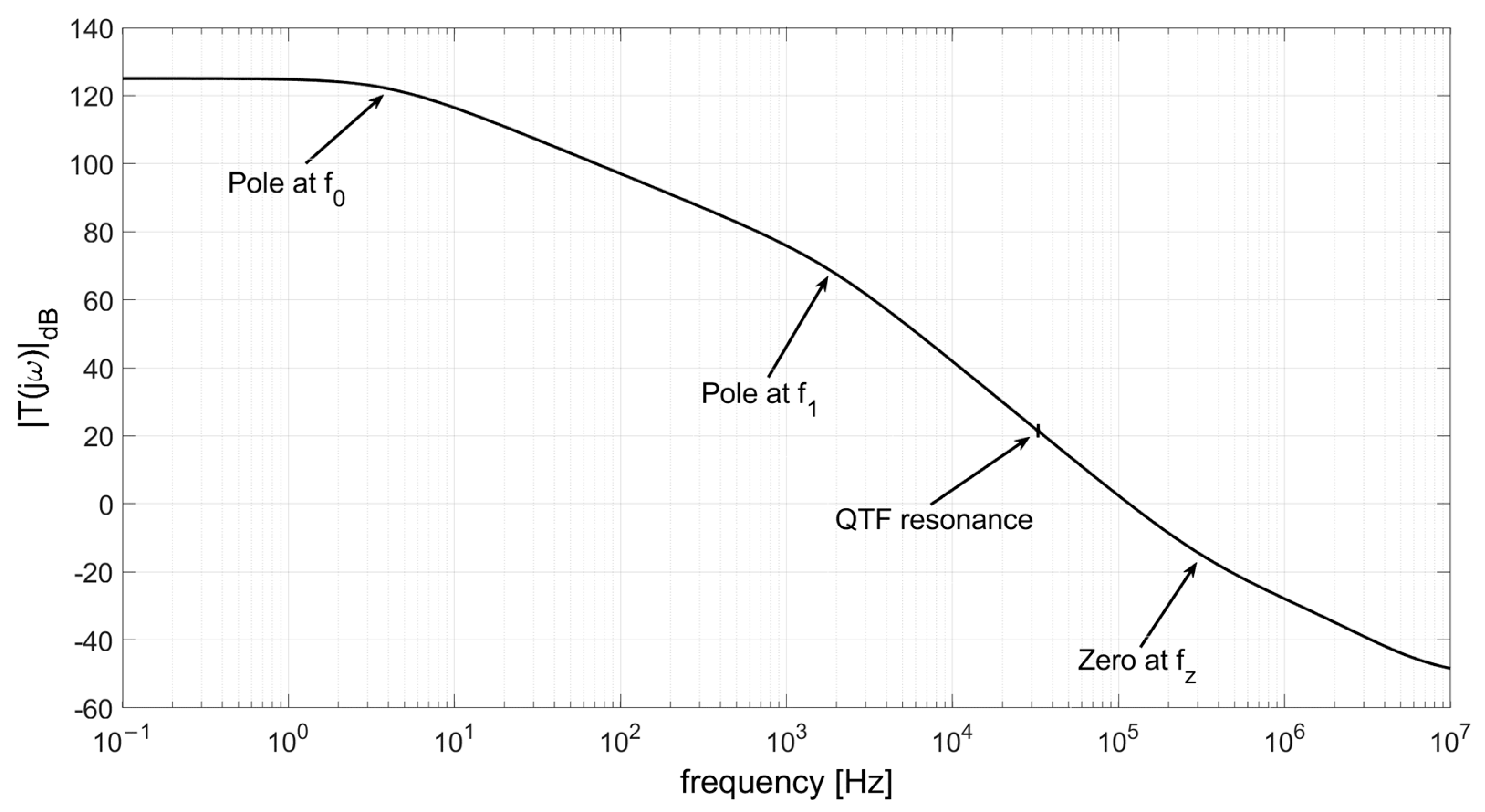
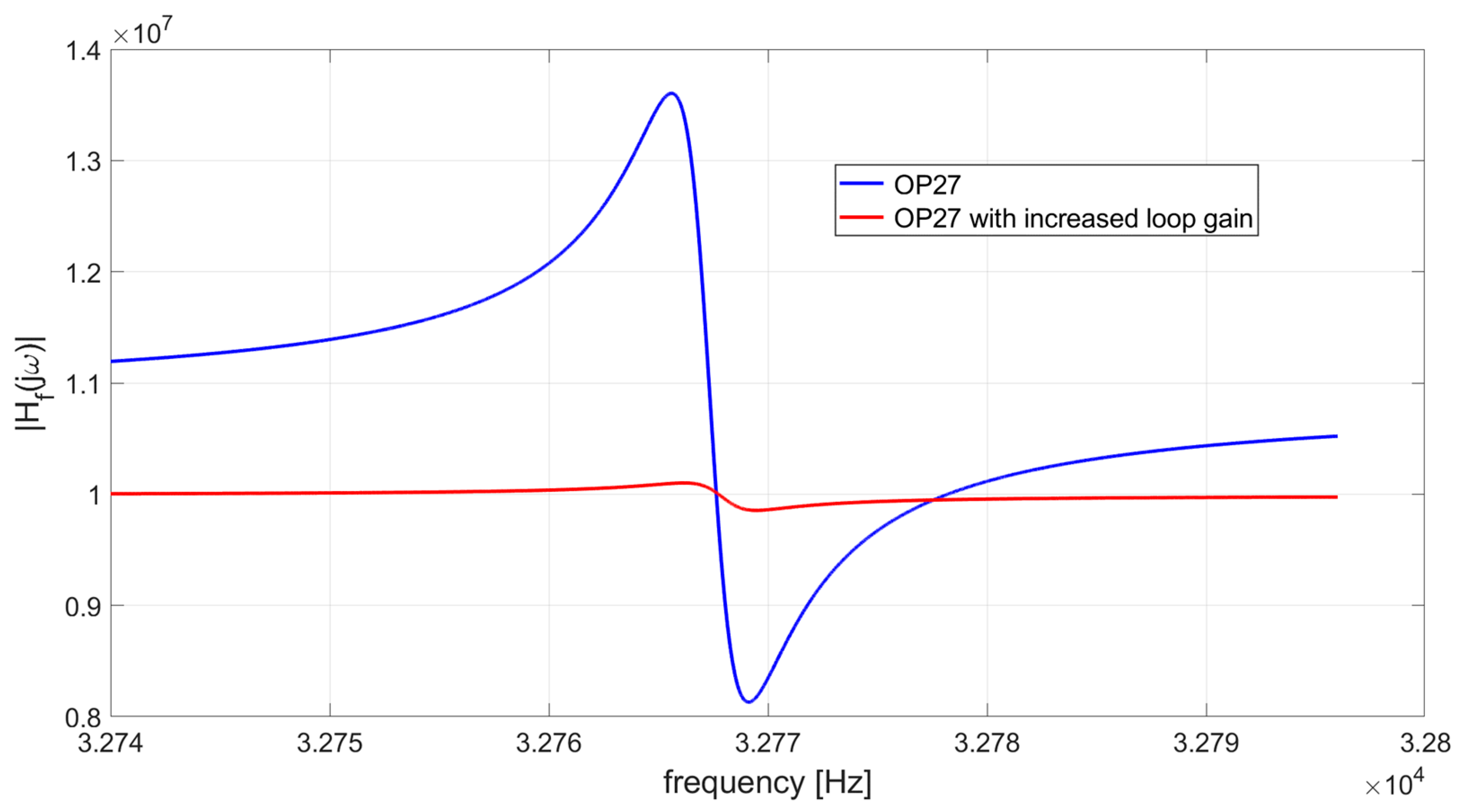
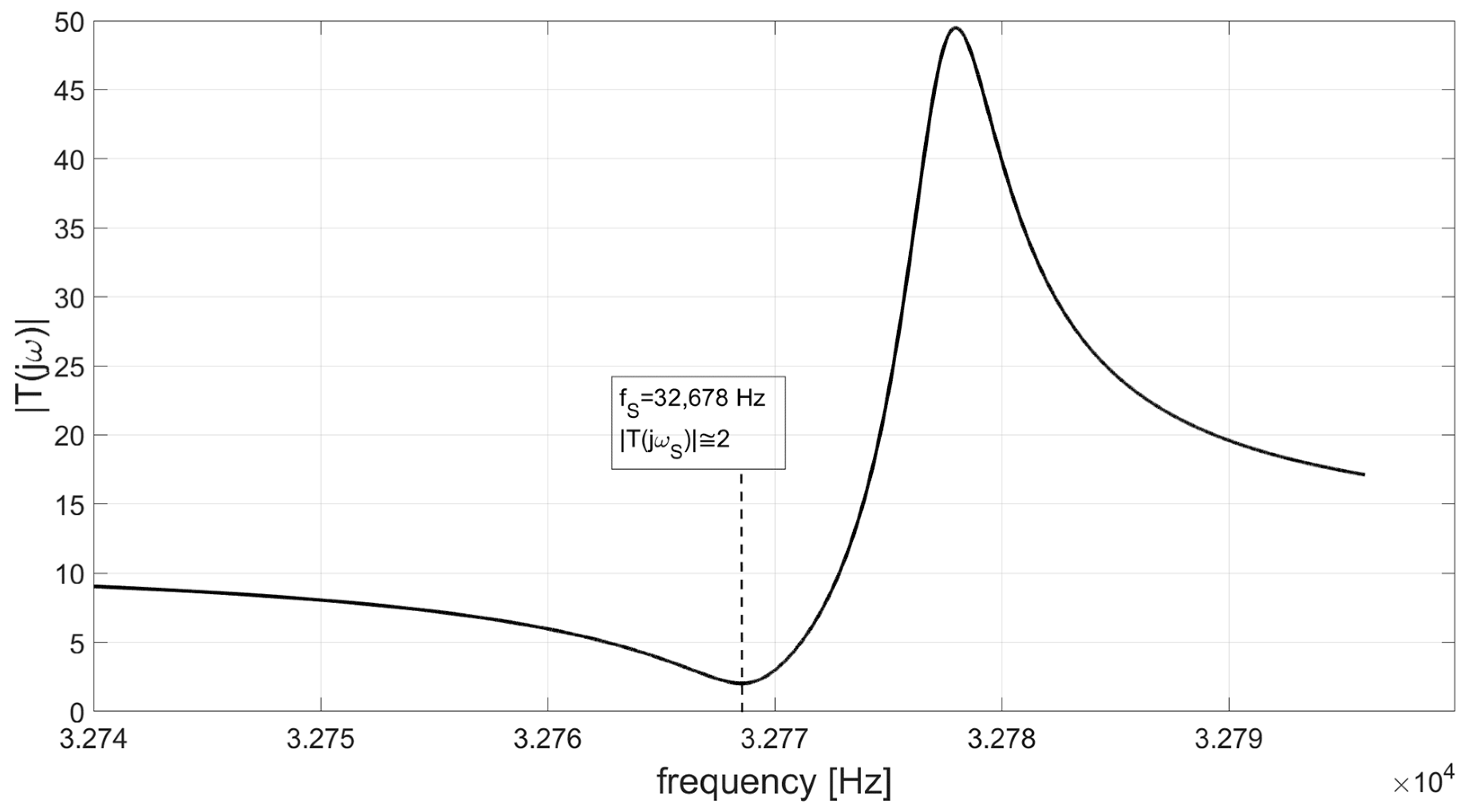
2.1. TIA Loop Gain as a Function of the OPAMP Gain–Bandwidth Product

To study the frequency response of the TIA shown in Figure 3, the QTF can be the described by means of the classic Butterworth–Van Dyke model—with a sinusoidal voltage source V_in inserted in series with the motional arm composed of R_P, C_S and L—as represented in Figure 4. Here, V_in represents the electric signal generated by the QTF when the sensor is excited by an acoustic stimulus, due to the piezoelectric effect. In Figure 4, the QTF model is coupled to the TIA, where the resistor R_F sets the closed loop gain of the circuit, C_F accounts for the parasitic capacitance in parallel to the feedback resistor, and C_IN is the input capacitance of the OPAMP.

A typical set of values for the passive components of the circuit in Figure 4 are reported in

Table 1. Values of the passive components of the circuit in Figure 4.

Parameter	Value
Cp	5 pF
CS	5.2424 fF
L	4.50 kH
Rp	92.65 kΩ
Cin	4 pF
RF	10 MΩ
CF	50 fF

. With these parameters, the series resonant frequency of the QTF ${\mathrm{f}}_{\mathrm{S}}=1/\left(2\mathsf{\pi }\sqrt{\mathrm{L}{\mathrm{C}}_{\mathrm{S}}}\right)$ is 32.768 kHz and its Q factor $1/\left({2\mathsf{\pi }\mathrm{f}}_{\mathrm{s}}{\mathrm{R}}_{\mathrm{p}}{\mathrm{C}}_{\mathrm{s}}\right)$ is about 10⁴. A conservative value of 50fF has been assumed for the parasitic capacitance C_F associated with a surface mount resistor [19]. As is well known, the noise contribution of the feedback resistor decreases for increasing values of R_F; thus, a large value of 10 MΩ has been considered [20,21]. The parameter values in Table 1 will be used for all the simulations except the input capacitance of the OPAMP, which depends on the specific considered device.

If the loop gain of the circuit in Figure 4 is very large (so that the inverting terminal of the OPAMP can be considered a good virtual ground), the total capacitance C_P + C_IN = C_PTOT is short-circuited and does not give any contribution to the transfer function H(jω) = V_OUT/V_IN of the circuit. The modulus squared of this transfer function is expressed as follows [21]:

$${\left|\mathrm{H}\left(\mathrm{j}\mathsf{\omega }\right)\right|}^2=\frac{{\left(\mathsf{\omega }{\mathrm{R}}_{\mathrm{F}}{\mathrm{C}}_{\mathrm{S}}\right)}^2}{{\left(1-\frac{{\mathsf{\omega }}^2}{{{\mathsf{\omega }}_{\mathrm{S}}}^2}\right)}^2+{\left(\mathsf{\omega }{\mathrm{R}}_{\mathrm{P}}{\mathrm{C}}_{\mathrm{S}}\right)}^2},$$

(2)

where ${\mathsf{\omega }}_{\mathrm{S}}=2\mathsf{\pi }{\mathrm{f}}_{\mathrm{S}}$. Because at this frequency the reactances of L and C_S are equal and opposite, they cancel each other, and the function |H(jω)|² exhibits a peak:

$${{\mathrm{H}}_{\mathrm{M}\mathrm{A}\mathrm{X}}}^2={\left|\mathrm{H}\left(\mathrm{j}{\mathsf{\omega }}_{\mathrm{S}}\right)\right|}^2={\left(\frac{{\mathrm{R}}_{\mathrm{F}}}{{\mathrm{R}}_{\mathrm{P}}}\right)}^2.$$

(3)

Note that C_F has been neglected in Equations (2) and (3), since ω_Z = 1/(R_FC_F) is much higher than ${\mathsf{\omega }}_{\mathrm{S}}$. We conclude that the most suitable operation frequency for the QEPAS system is the series resonant frequency of the QTF, where the response of the circuit to an acoustic excitation is maximized.

As already pointed out, Equations (2) and (3) hold true only if the loop gain T of the circuit is much greater than unity. Thus, it is important to evaluate this parameter around the series resonant frequency of the QTF in order to understand the conditions which must be fulfilled to validate the above analysis. The transfer function T(s), can be obtained by cutting the feedback loop at the inverting input of the OPAMP and evaluating the gain experienced by a signal which runs through the whole loop. This is given by the product of the differential gain of the OPAMP A_DM(s) and the voltage divider formed by the impedance of the QTF, Z_QTF as well as the feedback impedance R_F//(1/sC_F):

$$\mathrm{T}\left(\mathrm{s}\right)={\mathrm{A}}_{\mathrm{D}\mathrm{M}}\left(\mathrm{s}\right)\frac{{\mathrm{Z}}_{\mathrm{Q}\mathrm{T}\mathrm{F}}}{{\mathrm{Z}}_{\mathrm{Q}\mathrm{T}\mathrm{F}}+\frac{{\mathrm{R}}_{\mathrm{F}}}{{1+\mathrm{s}\mathrm{R}}_{\mathrm{F}}{\mathrm{C}}_{\mathrm{F}}}}.$$

(4)

To take into account the load effect of the input capacitance of the OPAMP C_in on the impedance of the QTF, the expression of Z_QTF must include the total capacitance C_PTOT and not only C_P. The following expression is obtained, neglecting C_S and C_F with respect to C_PTOT:

$$\mathrm{T}\left(\mathrm{s}\right)\cong {\mathrm{A}}_{\mathrm{D}\mathrm{M}}\left(\mathrm{s}\right)\frac{\left(1+\mathrm{s}{\mathrm{R}}_{\mathrm{F}}{\mathrm{C}}_{\mathrm{F}}\right)\left({\mathrm{s}}^2\mathrm{L}{\mathrm{C}}_{\mathrm{S}}+\mathrm{s}{\mathrm{R}}_{\mathrm{F}}{\mathrm{C}}_{\mathrm{S}}+1\right)}{{\mathrm{s}}^3\mathrm{L}{{\mathrm{R}}_{\mathrm{F}}\mathrm{C}}_{\mathrm{S}}{\mathrm{C}}_{\mathrm{P}\mathrm{T}\mathrm{O}\mathrm{T}}+{\mathrm{s}}^2\left(\mathrm{L}{\mathrm{C}}_{\mathrm{S}}+{{\mathrm{R}}_{\mathrm{P}}\mathrm{R}}_{\mathrm{F}}{\mathrm{C}}_{\mathrm{S}}{\mathrm{C}}_{\mathrm{P}\mathrm{T}\mathrm{O}\mathrm{T}}\right)+\mathrm{s}\left[{{\mathrm{R}}_{\mathrm{P}}\mathrm{C}}_{\mathrm{S}}+{\mathrm{R}}_{\mathrm{F}}{\mathrm{C}}_{\mathrm{P}\mathrm{T}\mathrm{O}\mathrm{T}}\right]+1}.$$

(5)

Typically, A_DM(s) is a single-pole transfer function with a very low cut-off frequency f₀, due to OPAMP internal compensation. For frequencies higher than the cut-off, the differential gain of the OPAMP can be expressed as a function of the frequency, as follows:

$${\mathrm{A}}_{\mathrm{D}\mathrm{M}}\left(\mathrm{j}\mathsf{\omega }\right)\cong \frac{{\mathrm{A}}_0}{\mathrm{j}\frac{\mathsf{\omega }}{{\mathsf{\omega }}_0}}=\frac{\mathrm{G}\mathrm{B}\mathrm{W}}{\mathrm{j}\mathsf{\omega }},$$

(6)

where A₀ is the DC gain of the amplifier and GWB = A₀·ω₀ is its gain–bandwidth product. The transfer function of Equation (5) contains a zero at ω_Z due to the presence of the small capacitance C_F, which makes the phase margin of the circuit acceptable.

If, for instance, we use the OP27 [11], an OPAMP with a gain–bandwidth product of about 8 MHz, the result of a broadband SPICE simulation of the magnitude of the loop gain |T(jω)| as a function of the frequency is shown in Figure 5.

Figure 5 has been generated by simulating 1000 points per decade, and as a consequence, the effects of the QTF resonance—confined in a very narrow band around 32.768 kHz—are barely visible. Instead, the main singularities of T(s) (i.e., the dominant pole of the OPAMP at f₀ ≅ 4 Hz, a low-frequency pole at f₁ ≅ 1/(2πR_FC_PTOT) ≅ 1.8 kHz, and the zero at f_Z = 1/(2πR_FC_F) ≅ 318 kHz) are clearly visible. We can conclude that due to the presence of the low-frequency poles located at f₀ and f₁, the magnitude of the loop gain around f_S is slightly more than 20 dB, despite the GBW of the OPAMP being about two orders of magnitude larger than the QTF resonant frequency.

Let us consider now what happens in the correspondence of the frequency f_S, which should be the optimal operating frequency for the QEPAS sensor. Here, the motional branch of the QTF reaches its minimum impedance and can be replaced by the only resistor R_P. With the typical values of the parameters we are considering, the frequency 1/(2πR_PC_PTOT) ≅ 180 kHz is quite large compared to f_S, so we can neglect the capacitance C_PTOT in parallel with R_P. Thus, the loop gain at f_S is simply evaluated as follows:

$$\mathrm{T}\left(\mathrm{j}{\mathsf{\omega }}_{\mathrm{S}}\right)\cong {\mathrm{A}}_{\mathrm{D}\mathrm{M}}\left(\mathrm{j}{\mathsf{\omega }}_{\mathrm{S}}\right)\frac{{\mathrm{R}}_{\mathrm{P}}}{{\mathrm{R}}_{\mathrm{F}}+{\mathrm{R}}_{\mathrm{P}}}\cong -\mathrm{j}\frac{\mathrm{G}\mathrm{B}\mathrm{W}}{{\mathsf{\omega }}_{\mathrm{S}}}\frac{{\mathrm{R}}_{\mathrm{P}}}{{\mathrm{R}}_{\mathrm{F}}}.$$

(7)

Equation (7) states that the value of |T(jω_S)| is obtained by multiplying the gain of the OPAMP at the resonant frequency of the QTF by the ratio R_P/R_F, which is very small in typical cases, as in ours. For instance, if we use the OP27, |T(jω_S)| is around 2.3 and the inverting input terminal of the OPAMP cannot be considered a good virtual ground at all. This invalidates Equations (2) and (3). An OPAMP with a GBW at least an order of magnitude higher would be needed to have a TIA with behavior closer to the ideal.

SPICE simulations of the TIA confirm this result. Figure 6 shows the amplitude of the loop gain of the circuit as a function of the frequency in a narrow band around the resonant frequency of the QTF. The value of |T(jω_S)| is around 2, which is very close to the above estimation.

The low value of the loop gain will cause deviations in the TIA response with respect to the ideal one. In turn, this modified behavior affects the choice of the optimal operating frequency for the application of the QEPAS technique, as will be discussed in the next section.

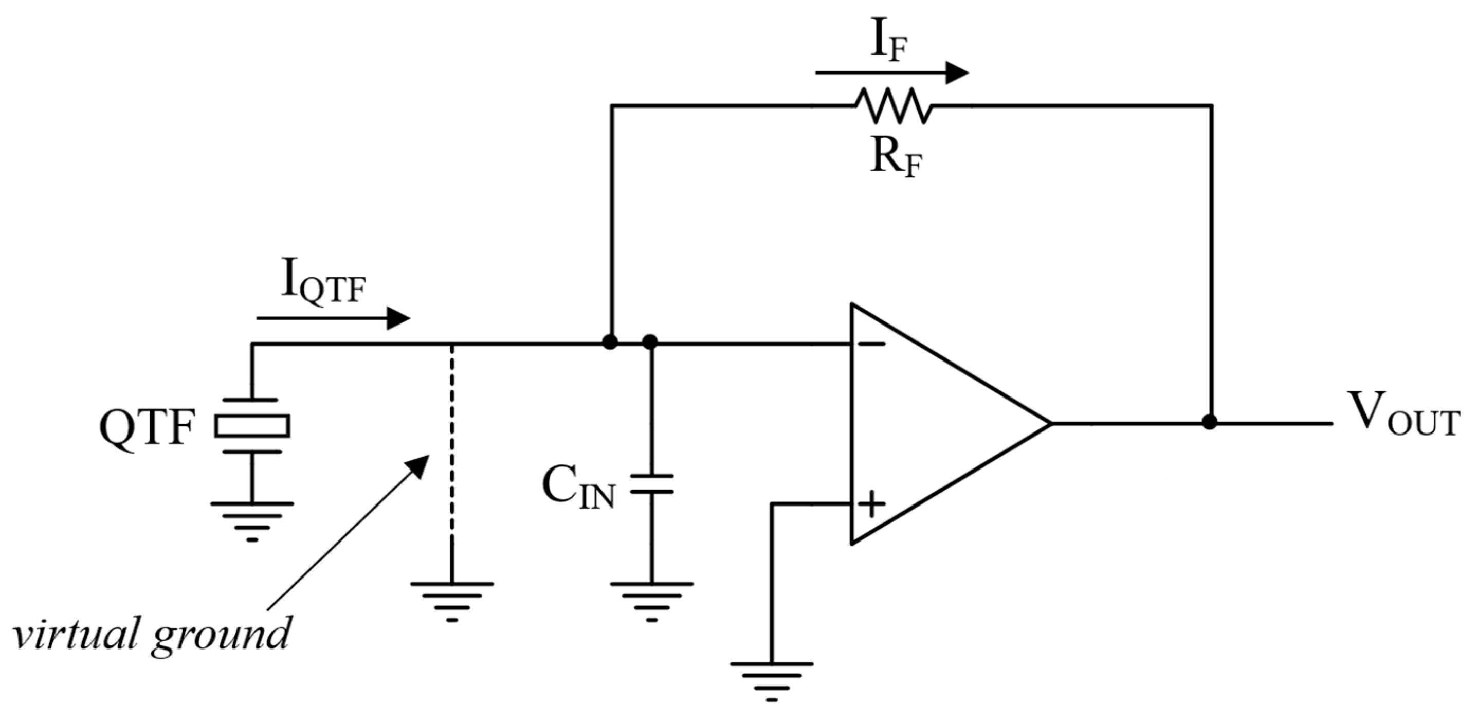
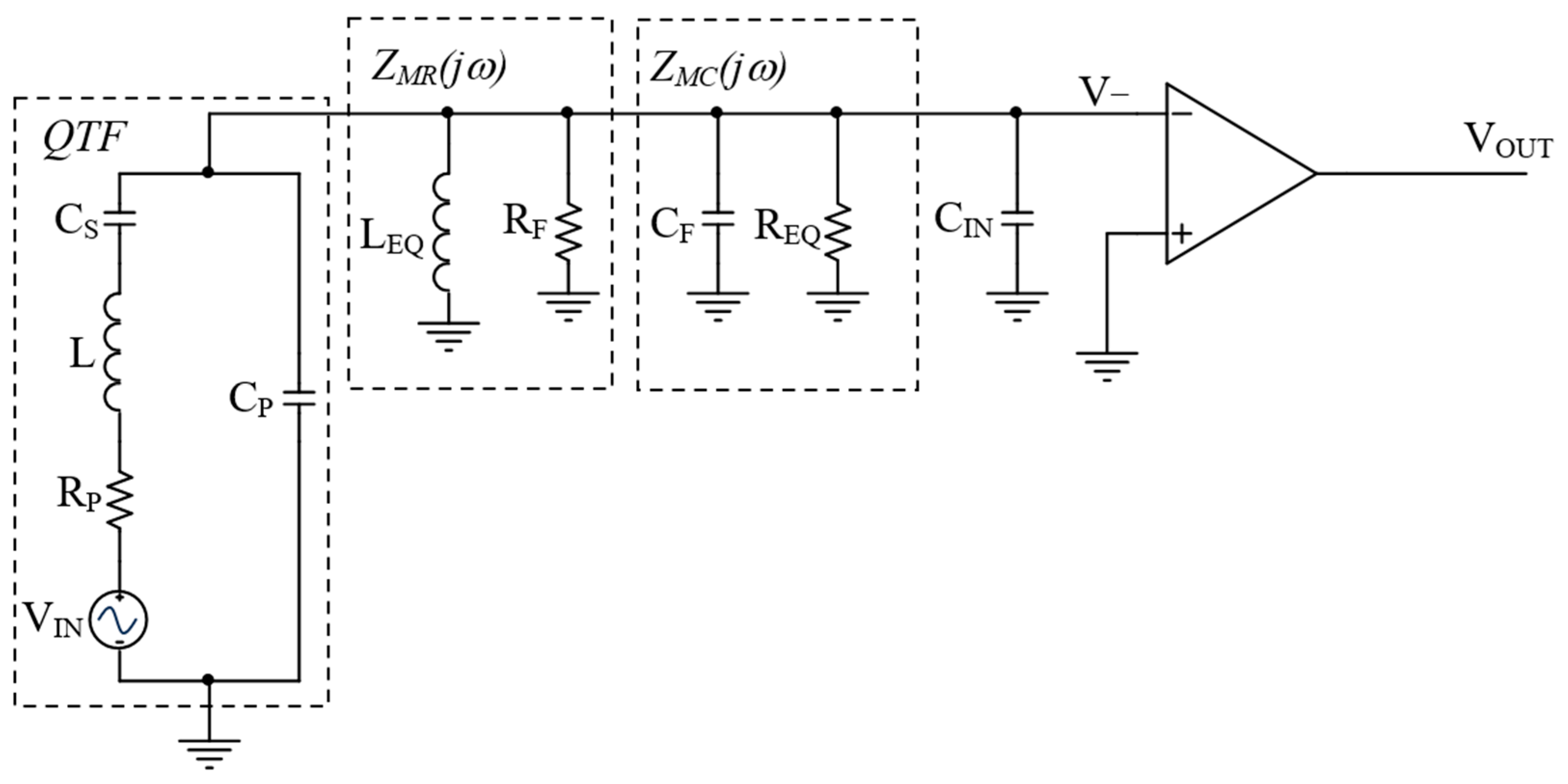
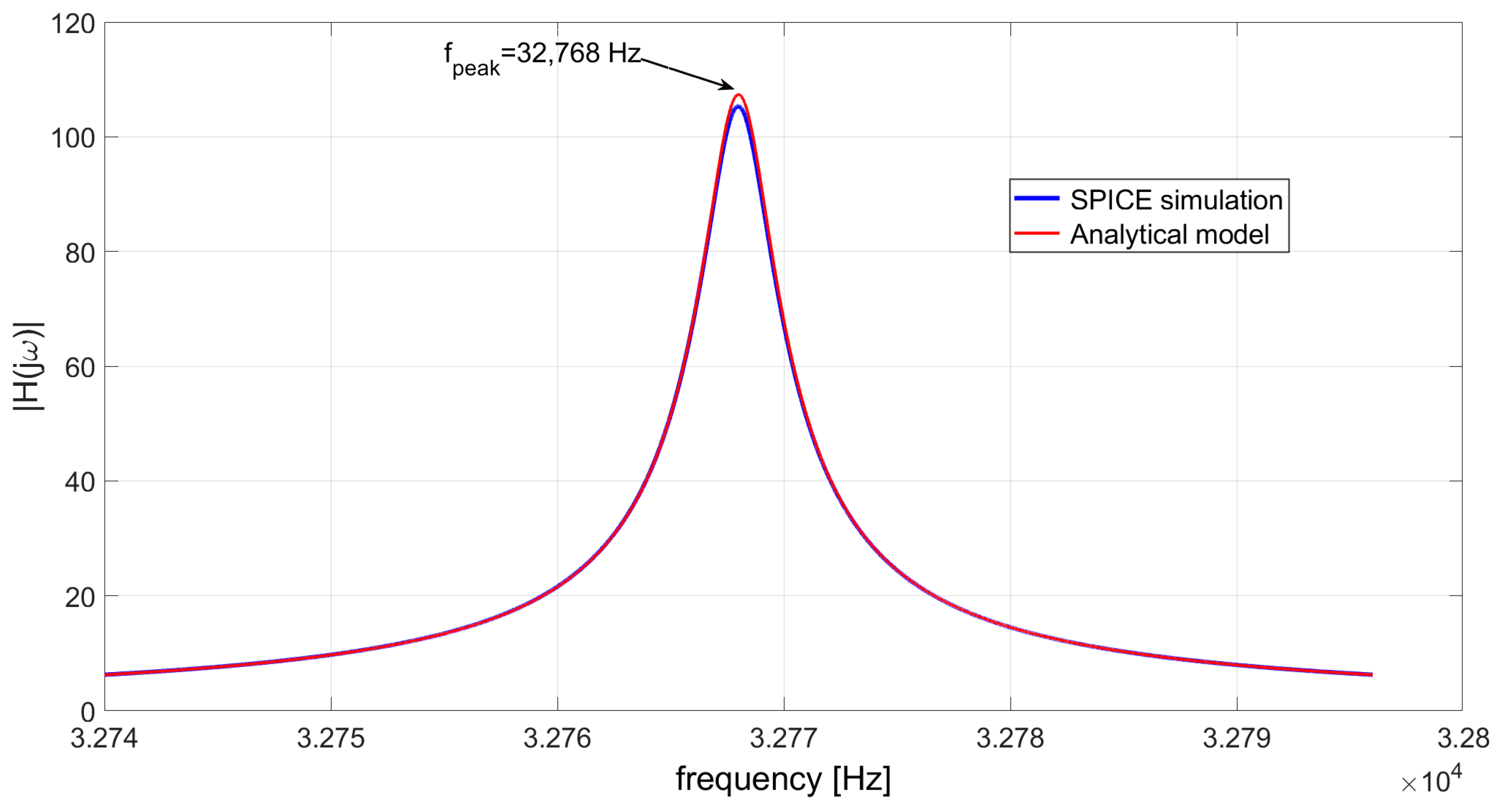
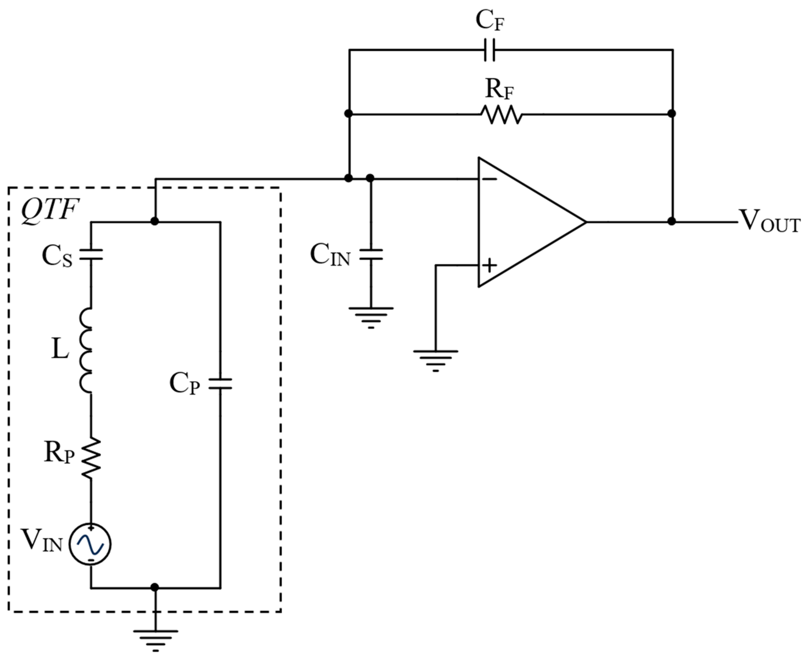
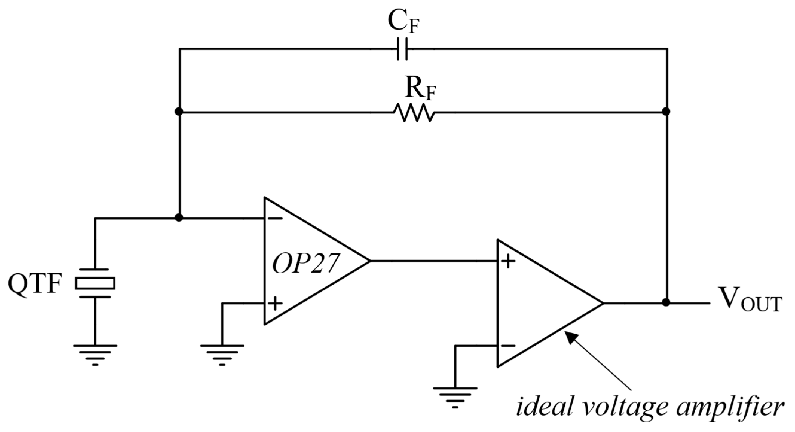
2.2. Closed-Loop Response of the TIA Coupled to the QTF

With a very low value of the loop gain |T(jω_S)|, the analysis of the closed-loop behavior of the circuit in Figure 4 cannot be carried out considering the presence of the virtual ground. The finite value of the OPAMP gain around the resonant frequency of the QTF must be necessarily taken into account. To study the circuit, we can apply Miller’s theorem [22] to the feedback impedance Z_F, composed by the parallel of the resistor R_F and the parasitic capacitor C_F. According to this theorem, an equivalent circuit of the TIA is created by replacing Z_F with an impedance Z_M1, placed between the inverting input of the OPAMP and ground, and an impedance Z_M2, connected between the OPAMP output node and ground:

$${\mathrm{Z}}_{\mathrm{M}1}\left(\mathrm{j}\mathsf{\omega }\right)=\frac{{\mathrm{Z}}_{\mathrm{F}}}{{1+\mathrm{A}}_{\mathrm{D}\mathrm{M}}\left(\mathrm{j}\mathsf{\omega }\right)}\hspace{1em}\hspace{1em}\hspace{1em}{\mathrm{Z}}_{\mathrm{M}2}\left(\mathrm{j}\mathsf{\omega }\right)=\frac{{\mathrm{Z}}_{\mathrm{F}}}{1+\frac{1}{{\mathrm{A}}_{\mathrm{D}\mathrm{M}}\left(\mathrm{j}\mathsf{\omega }\right)}}.$$

(8)

Due to the very low output impedance of the OPAMP, Z_M2 cannot affect the behavior of the circuit and can be omitted. Instead, for what concerns Z_M1, there are two contributions Z_MR and Z_MC in parallel, coming from R_F and C_F, respectively. According to Equation (6), Z_MR(jω) is expressed as follows:

$${\mathrm{Z}}_{\mathrm{M}\mathrm{R}}\left(\mathrm{j}\mathsf{\omega }\right)\cong \frac{{\mathrm{R}}_{\mathrm{F}}}{1+\frac{\mathrm{G}\mathrm{B}\mathrm{W}}{\mathrm{j}\mathsf{\omega }}}=\frac{{\mathrm{R}}_{\mathrm{F}}\frac{\mathrm{j}\mathsf{\omega }}{\mathrm{G}\mathrm{B}\mathrm{W}}}{1+\frac{\mathrm{j}\mathsf{\omega }}{\mathrm{G}\mathrm{B}\mathrm{W}}}$$

(9)

and can be considered as the parallel of the resistor R_F with an inductor L_EQ = R_F/GBW.

The contribution of the parasitic capacitance to the input Miller’s impedance is as follows:

$${\mathrm{Z}}_{\mathrm{M}\mathrm{C}}\left(\mathrm{j}\mathsf{\omega }\right)\cong \frac{1}{\mathrm{j}\mathsf{\omega }{\mathrm{C}}_{\mathrm{F}}\left(1+\frac{\mathrm{G}\mathrm{B}\mathrm{W}}{\mathrm{j}\mathsf{\omega }}\right)}=\frac{1}{\mathrm{j}\mathsf{\omega }{\mathrm{C}}_{\mathrm{F}}+{\mathrm{C}}_{\mathrm{F}}\mathrm{G}\mathrm{B}\mathrm{W}}.$$

(10)

Z_MC can be considered the parallel of the capacitance C_F with a resistor R_EQ = 1/(C_F⋅GBW). With the typical values of the parameters shown in Table 1, using the OP27 (GBW ≅ 2π⋅8 × 10⁶), we obtain L_EQ ≅ 0.2 H and R_EQ ≅ 400 kΩ. Figure 7 shows the equivalent circuit of the TIA after the application of Miller’s theorem.

Note that C_F << C_PTOT and R_F>>R_EQ can be neglected. Moreover, the resonant frequencies of the circuit in Figure 7 are poorly affected by the resistors R_P and R_EQ; thus, in order to find their location, it is sufficient to consider the simplified circuit shown in Figure 8.

The resonant frequency of the parallel L_EQ-C_PTOT is placed at

$${\mathrm{f}}_{\mathrm{E}}=\frac{1}{2\mathsf{\pi }\sqrt{{{\mathrm{L}}_{\mathrm{E}\mathrm{Q}}\mathrm{C}}_{\mathrm{P}\mathrm{T}\mathrm{O}\mathrm{T}}}}\cong 120 \mathrm{k}\mathrm{H}\mathrm{z},$$

which is quite a bit higher than f_S. As a consequence, around f_S, this network exhibits an inductive behavior, which slightly shifts the peak of the transfer function |H(jω)| with respect to the expected value, f_S. In fact, since around f_S the parallel L_EQ-C_PTOT is equivalent to a frequency-dependent inductor L_X(ω), the transfer function of the circuit in Figure 8 is as follows:

$$\frac{{\mathrm{V}}_{-}}{{\mathrm{V}}_{\mathrm{I}\mathrm{N}}}\cong \frac{\mathrm{j}\mathsf{\omega }{\mathrm{L}}_{\mathrm{X}}\left(\mathsf{\omega }\right)}{\mathrm{j}\mathsf{\omega }\left({\mathrm{L}}_{\mathrm{X}}\left(\mathsf{\omega }\right)+\mathrm{L}\right)+\frac{1}{\mathrm{j}\mathsf{\omega }{\mathrm{C}}_{\mathrm{S}}}}=-\frac{{\mathsf{\omega }}^2{\mathrm{C}}_{\mathrm{S}}{\mathrm{L}}_{\mathrm{X}}\left(\mathsf{\omega }\right)}{1-{\mathsf{\omega }}^2{\mathrm{C}}_{\mathrm{S}}\left({\mathrm{L}}_{\mathrm{X}}\left(\mathsf{\omega }\right)+\mathrm{L}\right)},$$

and its peak is located at the frequency f_peak, lower than the series resonant frequency of the QTF:

$${\mathrm{f}}_{\mathrm{p}\mathrm{e}\mathrm{a}\mathrm{k}}=\frac{1}{2\mathsf{\pi }\sqrt{{\mathrm{C}}_{\mathrm{S}}\left({\mathrm{L}}_{\mathrm{X}}\left(\mathsf{\omega }\right)+\mathrm{L}\right)}}<{\mathrm{f}}_{\mathrm{S}}.$$

(11)

Of course, the complete transfer function H(jω) = V_OUT/V_IN of the circuit in Figure 7 is obtained by multiplying V₋/V_IN by the open loop gain of the OPAMP A_DM(jω).

3. Results

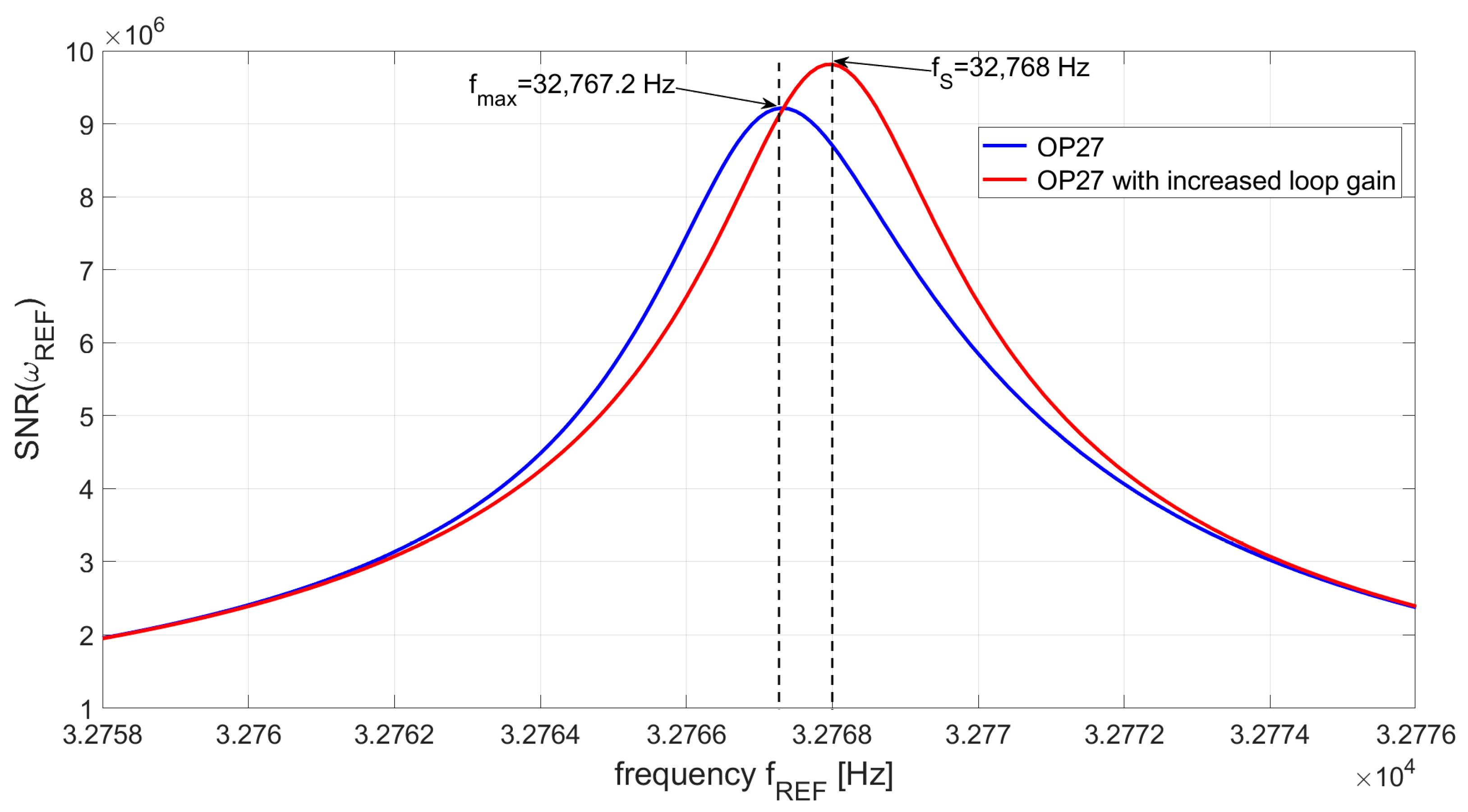
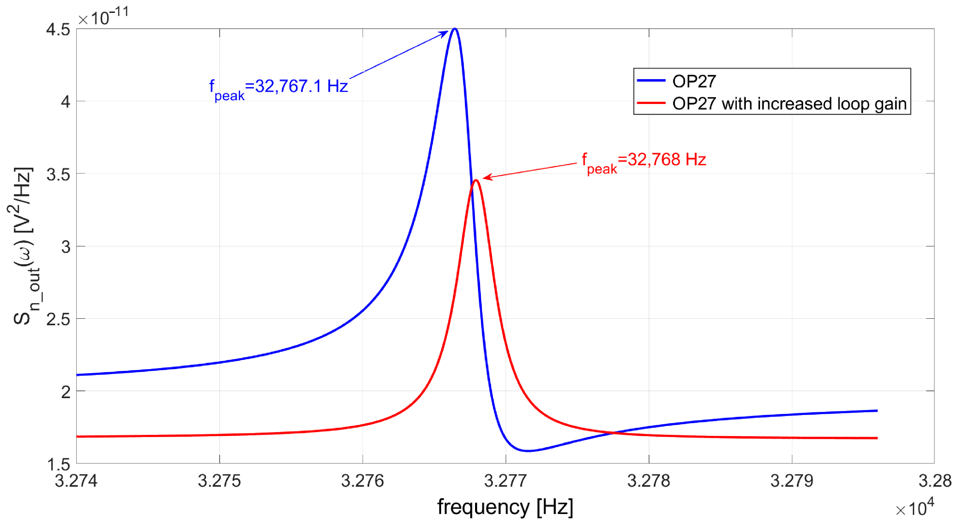
3.1. Shift of the Peak Frequency

The shift of the peak frequency towards lower values, expressed by Equation (11), is confirmed by SPICE simulations of the TIA. Figure 9 shows the behavior of the modulus of the transfer function H(jω) for three different OPAMPs, listed in

Table 2. OPAMP models used for the SPICE simulations.

OPAMP	Gain–Bandwidth Product [MHz]	Peak Frequency fpeak [Hz]
OP27	8	32,767.1
TL071	3	32,766.2
AD8067	300	32,768.0

together with their gain–bandwidth products and the peak frequency f_peak obtained in simulation.

Table 2 shows that when the large bandwidth OPAMP AD8067 is used, the peak frequency of the TIA response coincides with the resonant frequency of the QTF, as expected. Instead, with the other two OPAMP models, the shift of f_peak with respect to f_S is apparent and is more pronounced for the slowest OPAMP, the TL071. This shift of about 0.9 Hz and 1.8 Hz for the OP27 and the TL071, respectively, can be significant in terms of performance of the QEPAS sensor. Note that if an external sine wave is applied to the QTF coupled to the TIA for the identification of the optimal operating frequency of the QEPAS sensor, as described in the Introduction, the result of the procedure will be always f_peak; this is different from f_S in cases in which a too slow OPAMP is used, such as the OP27 or the TL071.

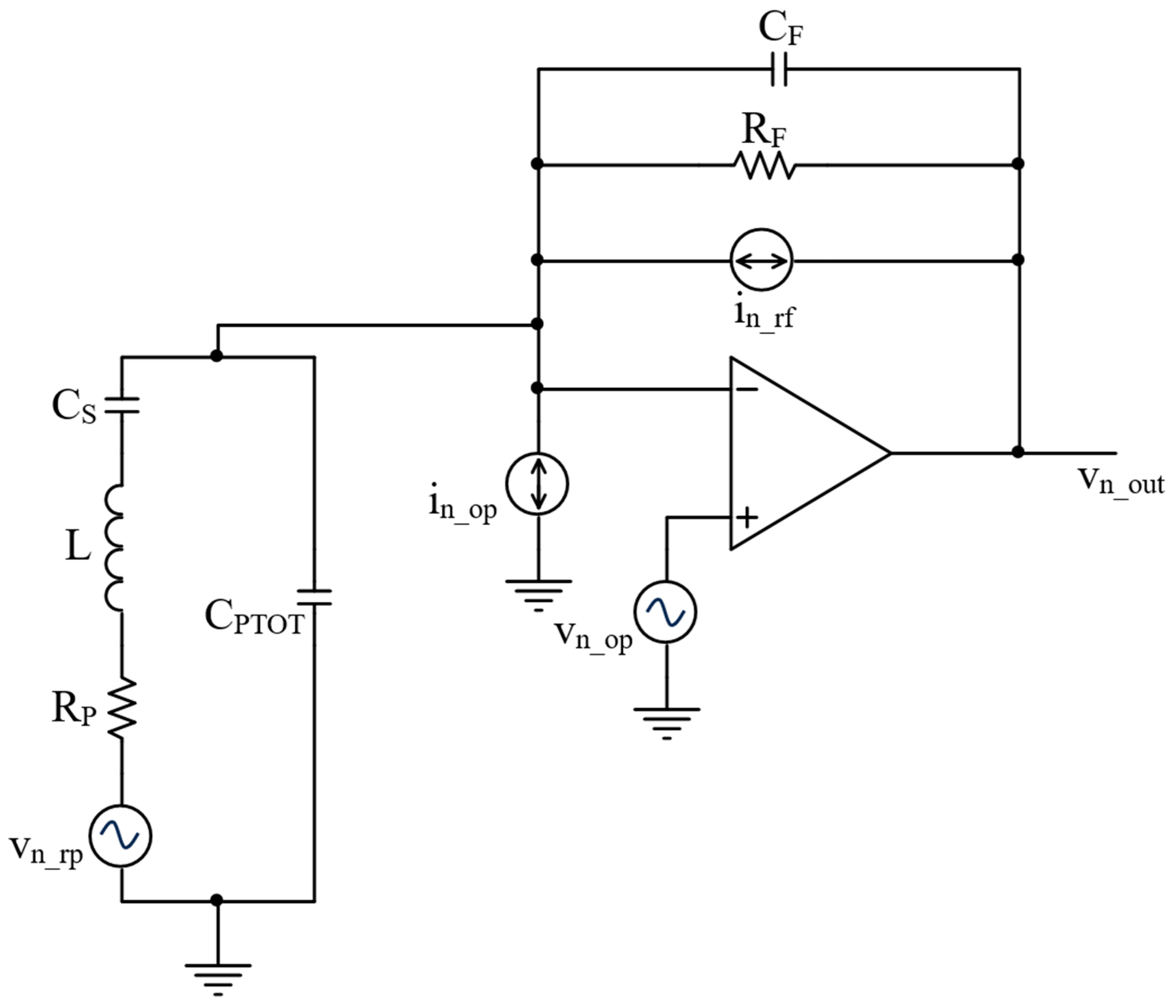
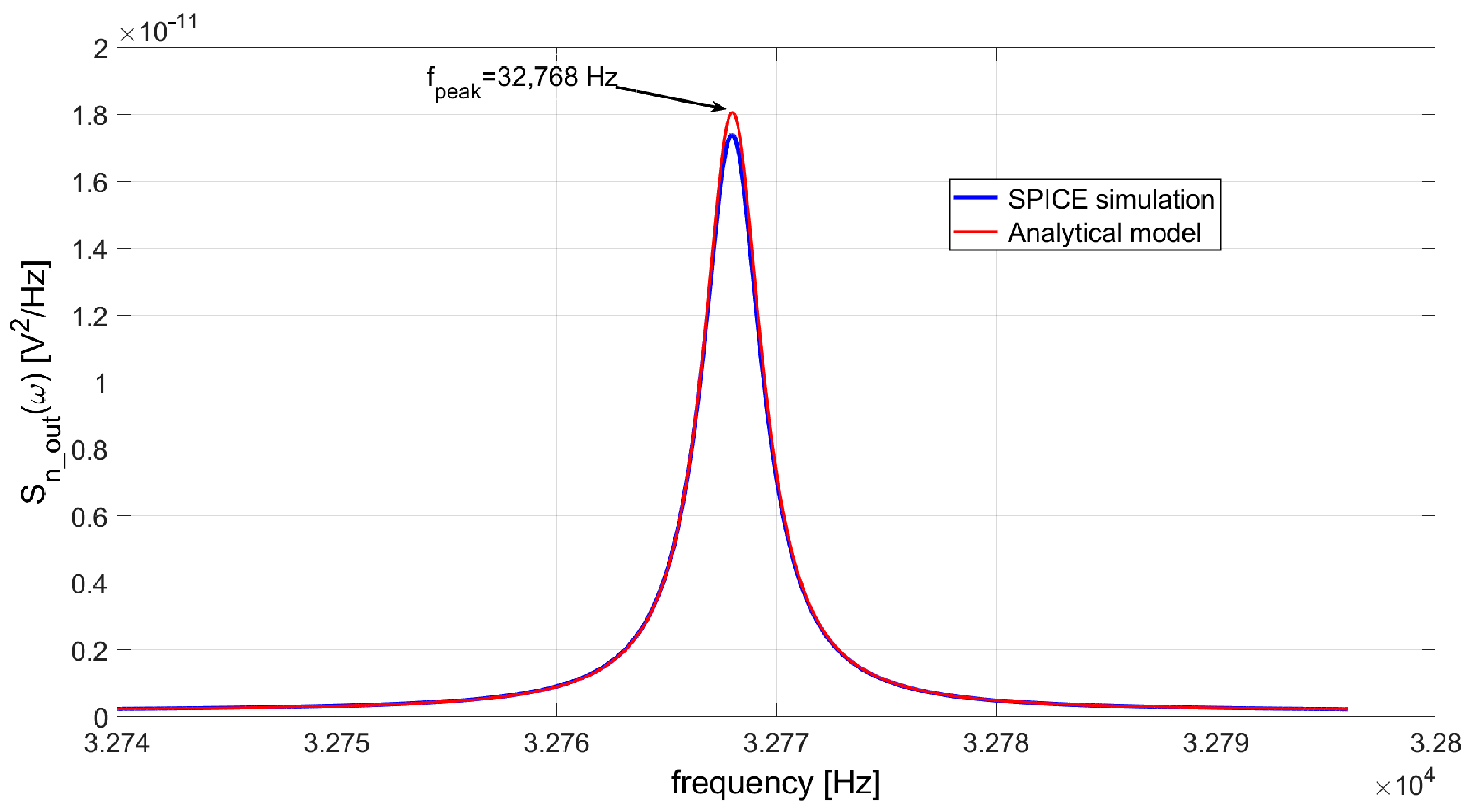
3.2. Effects of the Limited GBW on the TIA Output Noise

To assess the performance of the TIA used as a front-end for the QTF in a QEPAS sensor, it is mandatory to study the signal-to-noise ratio (SNR) obtained at its output. The main noise sources in the circuit of Figure 4 are the thermal noise of the resistors R_P and R_F, v_{n_rp} and i_{n_rf}, respectively, and the equivalent input noise sources of the OPAMP, v_{n_op} and i_{n_op}, as represented in Figure 10. The contributions of these noise sources to the total output noise power spectral density at the series resonant frequency of the QTF are well known in the literature, and the dominant contribution is recognized to be the thermal noise of the resistor R_P [20,23,24]. In the following, the behavior of the noise power spectral density as a function of the frequency is studied, and the effects of the missing virtual ground at the OPAMP input due to its limited GBW are investigated.

The total power spectral density of the output noise S_{n_out} is obtained by summing the contributions given by the power spectral densities of the noise sources in Figure 10, weighted by the corresponding transfer functions:

$${\mathrm{S}}_{\mathrm{n}\_\mathrm{o}\mathrm{u}\mathrm{t}}\left(\mathsf{\omega }\right)={\mathrm{S}}_{\mathrm{n}\_\mathrm{r}\mathrm{p}}{\left|\mathrm{H}\left(\mathrm{j}\mathsf{\omega }\right)\right|}^2+\left({\mathrm{S}}_{\mathrm{n}\_\mathrm{r}\mathrm{f}}+{{\mathrm{i}}_{\mathrm{n}\_\mathrm{o}\mathrm{p}}}^2\right){\left|{\mathrm{H}}_{\mathrm{f}}\left(\mathrm{j}\mathsf{\omega }\right)\right|}^2+{{\mathrm{v}}_{\mathrm{n}\_\mathrm{o}\mathrm{p}}}^2{\left|{\mathrm{H}}_{\mathrm{v}\mathrm{n}\_\mathrm{o}\mathrm{p}}\left(\mathrm{j}\mathsf{\omega }\right)\right|}^2,$$

(12)

where

$${\mathrm{S}}_{\mathrm{n}\_\mathrm{r}\mathrm{p}}=4\mathrm{k}\mathrm{T}{\mathrm{R}}_{\mathrm{P}},\hspace{1em}\hspace{1em}{\mathrm{S}}_{\mathrm{n}\_\mathrm{r}\mathrm{f}}=\frac{4\mathrm{k}\mathrm{T}}{{\mathrm{R}}_{\mathrm{F}}},$$

and k is the Boltzmann constant and T the absolute temperature.

If the gain–bandwidth product of the OPAMP is large enough and its inverting input terminal can be considered a good virtual ground, |H(jω)|² is given by Equation (2), |H_f(jω)|² ≅ R_F², and

$${\left|{\mathrm{H}}_{\mathrm{v}\mathrm{n}\_\mathrm{o}\mathrm{p}}\left(\mathrm{j}\mathsf{\omega }\right)\right|}^2=\frac{{\left(1-\frac{{\mathsf{\omega }}^2}{{{\mathsf{\omega }}_{\mathrm{R}}}^2}\right)}^2+{\mathsf{\omega }}^2{\left({\mathrm{R}}_{\mathrm{P}}{\mathrm{C}}_{\mathrm{S}}+{\mathrm{R}}_{\mathrm{F}}\left({\mathrm{C}}_{\mathrm{S}}+{\mathrm{C}}_{\mathrm{P}\mathrm{T}\mathrm{O}\mathrm{T}}\right)\left(1-\frac{{\mathsf{\omega }}^2}{{{\mathsf{\omega }}_{\mathrm{P}}}^2}\right)\right)}^2}{{\left(1-\frac{{\mathsf{\omega }}^2}{{{\mathsf{\omega }}_{\mathrm{S}}}^2}\right)}^2+{\mathsf{\omega }}^2{{\mathrm{R}}_{\mathrm{P}}}^2{{\mathrm{C}}_{\mathrm{S}}}^2},$$

where ${\mathsf{\omega }}_{\mathrm{R}}=1/\sqrt{\mathrm{L}{\mathrm{C}}_{\mathrm{S}}+{\mathrm{R}}_{\mathrm{P}}{\mathrm{R}}_{\mathrm{F}}{\mathrm{C}}_{\mathrm{S}}{\mathrm{C}}_{\mathrm{P}\mathrm{T}\mathrm{O}\mathrm{T}}}$ and ${\mathsf{\omega }}_{\mathrm{P}}=1/\sqrt{\mathrm{L}{\mathrm{C}}_{\mathrm{S}}{\mathrm{C}}_{\mathrm{P}\mathrm{T}\mathrm{O}\mathrm{T}}/\left({\mathrm{C}}_{\mathrm{S}}+{\mathrm{C}}_{\mathrm{P}\mathrm{T}\mathrm{O}\mathrm{T}}\right)}$ [21].

A comparison between the results obtained with SPICE simulations and the analytical model confirms the validity of Equations (2) and (12). Figure 11 shows the modulus of the TIA transfer function |H(jω)|, whereas Figure 12 displays the total output noise power spectral density of the circuit S_{n_out}(ω), when the AD8067 is used, in which case the OPAMP inverting input can be considered a good virtual ground. In the analytical model, the values of the equivalent input noise sources of the OPAMP, i_{n_op} = 0.6 fA/√Hz and v_{n_op} = 6.6 nV/√Hz, have been derived from its data sheet. Moreover, preliminary simulations have been carried out to validate the noise behavior of the SPICE model of the OPAMPs considered in this study in order to guarantee that they describe the noise behavior of the amplifiers consistently with their data sheet. The parameters of the QTF model are the same as reported in Table 1. The analytical model just slightly overestimates the results provided by SPICE simulations, but the frequency f_peak coincides exactly with the series resonant frequency of the QTF f_S = 32,768 Hz, as expected.

If an OPAMP with a low GBW is used in the TIA, the noise transfer functions which appear in Equation (12) are affected by the missing virtual ground at the inverting input of the OPAMP, exactly as happens to |H(jω)|. If, for instance, we consider the OP27 and an OPAMP with the same input equivalent noise sources and the same input capacitance C_IN, but much larger GBW, we will observe a different frequency behavior of all the noise contributions in Equation (12). Such an OPAMP can be obtained in simulation by inserting an ideal voltage amplifier with gain equal to 20 into the feedback loop at the output of the OP27, as depicted in Figure 13.

Figure 14 shows a comparison between the total output noise power spectral density S_{n_out} of the TIA, achieved using the OP27 and an equivalent OPAMP with a GBW increased by a factor of 20 as shown in Figure 13.

It is apparent from Figure 14 that the behavior of S_{n_out} as a function of frequency is completely different in the two cases, which differ only in the GBW of the OPAMP. In particular, as illustrated by Figure 15, the transfer function H_f(jω) is strongly affected by the absence of a good virtual ground, as well as the contributions to the total output noise due to the equivalent input current noise of the OPAMP and the feedback resistor.

As a consequence, the behavior of the SNR at the output of the QEPAS sensor will also be dependent on the GBW of the OPAMP used in the QTF preamplifier as well as its noise performance.

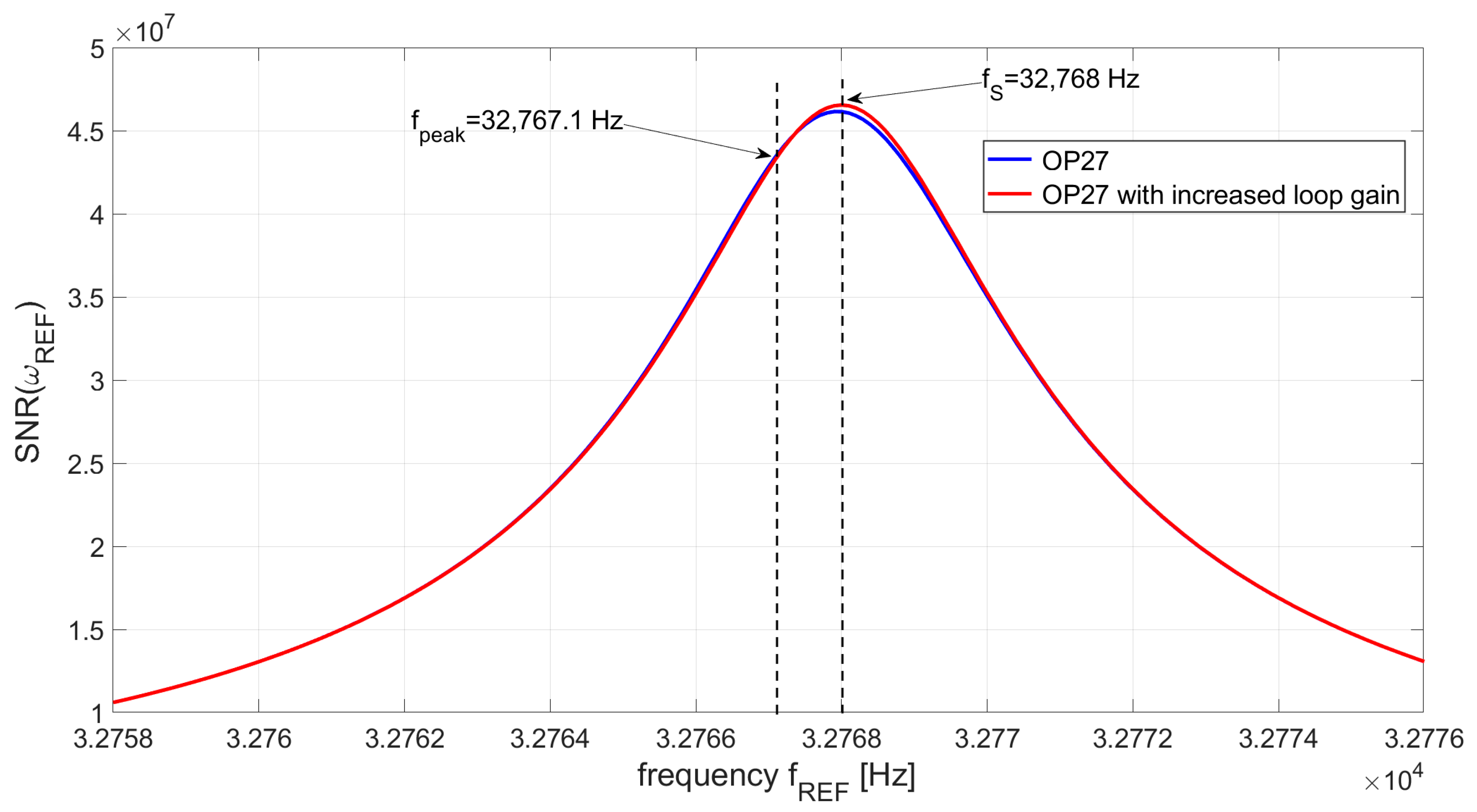
3.3. Evaluation of the SNR and Effects of the Limited GBW

For the evaluation of the SNR at the output of the QEPAS sensor, the function of the LIA can be considered equivalent to a band-pass filter with narrow bandwidth BW, centered at its reference frequency f_REF [21,25]. Thus, assuming a unity amplitude for the input signal V_IN, the SNR at the output of the LIA can be defined as follows:

$$\mathrm{S}\mathrm{N}\mathrm{R}\left({\mathsf{\omega }}_{\mathrm{R}\mathrm{E}\mathrm{F}}\right)=\frac{{\left|\mathrm{H}\left(\mathrm{j}{\mathsf{\omega }}_{\mathrm{R}\mathrm{E}\mathrm{F}}\right)\right|}^2}{{{\mathrm{V}}_{\mathrm{n}\_\mathrm{o}\mathrm{u}\mathrm{t}}\left({\mathsf{\omega }}_{\mathrm{R}\mathrm{E}\mathrm{F}}\right)}^2}=\frac{{\left|\mathrm{H}\left(\mathrm{j}{\mathsf{\omega }}_{\mathrm{R}\mathrm{E}\mathrm{F}}\right)\right|}^2}{{\int }_{-\mathrm{\infty }}^{\mathrm{\infty }}{\mathrm{S}}_{\mathrm{n}\_\mathrm{o}\mathrm{u}\mathrm{t}}\left(\mathsf{\omega }\right){\left|{\mathrm{H}}_{\mathrm{L}\mathrm{I}\mathrm{A}}\left(\mathrm{j}\mathsf{\omega }\right)\right|}^2\mathrm{d}\mathsf{\omega }},$$

(13)

where V_{n_out} is the rms value of the output noise, ω_REF = 2πf_REF, and

$${\mathrm{H}}_{\mathrm{L}\mathrm{I}\mathrm{A}}\left(\mathrm{j}\mathsf{\omega }\right)=\frac{\mathrm{j}\mathsf{\omega }\frac{{\mathsf{\omega }}_{\mathrm{R}\mathrm{E}\mathrm{F}}}{{\mathrm{Q}}_{\mathrm{f}\mathrm{i}\mathrm{l}\mathrm{t}}}}{{\mathsf{\omega }}_{\mathrm{R}\mathrm{E}\mathrm{F}}^2-{\mathsf{\omega }}^2+\mathrm{j}\mathsf{\omega }\frac{{\mathsf{\omega }}_{\mathrm{R}\mathrm{E}\mathrm{F}}}{{\mathrm{Q}}_{\mathrm{f}\mathrm{i}\mathrm{l}\mathrm{t}}}}$$

is the response of a biquadratic band-pass filter with a center frequency f_REF and bandwidth BW = ω_REF/Q_filt, used to simulate the LIA function.

If we want to enhance noise rejection, the bandwidth of the LIA filter must be extremely narrow, i.e., the LIA integration time must be very large. As a consequence, in practice, the squared rms output noise V_{n_out}(ω_REF)² is proportional to the noise power spectral density S_{n_out}(ω_REF) [11], and the SNR can be expressed as:

$$\begin{array}{ll}\mathrm{S}\mathrm{N}\mathrm{R}\left({\mathsf{\omega }}_{\mathrm{R}\mathrm{E}\mathrm{F}}\right)\propto & \frac{{\left|\mathrm{H}\left(\mathrm{j}{\mathsf{\omega }}_{\mathrm{R}\mathrm{E}\mathrm{F}}\right)\right|}^2}{{\mathrm{S}}_{{\mathrm{n}}_{\mathrm{o}\mathrm{u}\mathrm{t}}}\left({\mathsf{\omega }}_{\mathrm{R}\mathrm{E}\mathrm{F}}\right)}=\\ & \hspace{1em}=\frac{1}{{\mathrm{S}}_{{\mathrm{n}}_{\mathrm{r}\mathrm{p}}}+\left({\mathrm{S}}_{{\mathrm{n}}_{\mathrm{r}\mathrm{f}}}+{{\mathrm{i}}_{{\mathrm{n}}_{\mathrm{o}\mathrm{p}}}}^2\right)\frac{{\left|{\mathrm{H}}_{\mathrm{f}}\left(\mathrm{j}{\mathsf{\omega }}_{\mathrm{R}\mathrm{E}\mathrm{F}}\right)\right|}^2}{{\left|\mathrm{H}\left(\mathrm{j}{\mathsf{\omega }}_{\mathrm{R}\mathrm{E}\mathrm{F}}\right)\right|}^2}+{{\mathrm{v}}_{{\mathrm{n}}_{\mathrm{o}\mathrm{p}}}}^2\frac{{\left|{\mathrm{H}}_{{\mathrm{v}\mathrm{n}}_{\mathrm{o}\mathrm{p}}}\left(\mathrm{j}{\mathsf{\omega }}_{\mathrm{R}\mathrm{E}\mathrm{F}}\right)\right|}^2}{{\left|\mathrm{H}\left(\mathrm{j}{\mathsf{\omega }}_{\mathrm{R}\mathrm{E}\mathrm{F}}\right)\right|}^2}}.\end{array}$$

(14)

Notice that, in Equation (14), the ratios |H_f(jω_REF)|²/|H(jω_REF)|² and |H_{vn_op}(jω_REF)|²/|H(jω_REF)|² are independent on the GBW of the OPAMP used in the TIA. In other words, if the loop gain of the circuit is increased by adding a gain stage in the feedback loop, as shown in Figure 13, to obtain Figure 14 and Figure 15, these ratios are unaffected due to the linearity of the system. Thus, Equation (14) states that the dependence of the SNR on the LIA reference frequency f_REF is not affected by the GBW of the OPAMP.

Extensive SPICE simulations have been carried out to support this conclusion. A band-pass filter with BW = 0.1 Hz has been cascaded to the same TIAs, based on the OPAMP OP27, used to reproduce Figure 14 and Figure 15. The SNR at the filter output, expressed by Equation (13), has been simulated by varying the center frequency of the filter by steps of 0.1 Hz, around the resonance of the QTF, in the interval from 32,758 Hz to 32,776 Hz.

Figure 16 shows the behavior of the SNR obtained with and without boosting the GBW of the OPAMP by means of an ideal voltage amplifier with a gain of 20. As expected, the increase in the loop gain of the TIA does not affect the behavior of the SNR too much; in particular, it does not modify the value of the reference frequency corresponding to the peak of the SNR, which remains almost coincident with the series resonant frequency of the QTF, f_S. This means that the optimal operating frequency for the QEPAS sensor is f_S, which is different from f_peak, i.e., the frequency where the peak of the signal is obtained, in case the OP27 is used for the TIA. As a consequence, if the QEPAS sensor is operated at the frequency f_peak, an appreciable penalty in terms of SNR results, as highlighted in Figure 16. Thus, we can conclude that for the very long integration time of the LIA, the use of a TIA realized with an OPAMP with limited GBW, like the OP27 or the TL071, leads to a nonoptimal choice of the operating frequency of the QEPAS sensor.

Since the shift of f_peak with respect to f_S increases for decreasing values of GBW, using an OPAMP such as the TL071 (GBW = 3 MHz) would result in larger penalties in terms of SNR, if the chosen operating frequency of the QEPAS sensor is f_peak instead of f_S.

When we need to increase the rate of the measurements, the bandwidth of the LIA filter must be increased as well. The noise power spectral density is integrated in a larger bandwidth around the LIA reference frequency, and the peak of the SNR at the LIA output tends to move close to the peak frequency of the signal f_peak; thus, the choice of the operating frequency of the QEPAS sensor is near to the optimal one. Nevertheless, the maximum SNR achievable is well below the one that can be obtained when keeping the same noise performance of the OPAMP but increasing its GBW so that the optimal operating frequency and the signal peak frequency f_peak both coincide with f_S. This is illustrated in Figure 17, where the simulated behavior of the SNR as a function of the LIA reference frequency is shown for a filter bandwidth of 3 Hz and a TIA based on the OPAMP OP27, both with and without boosting of the loop gain.

If the sheer OP27 is used, the frequency corresponding to the peak of the SNR is f_max = 32,768.2 Hz, very close to f_peak = 32,768.1 Hz, but the maximum value of the SNR is about 9.2 × 10⁶, which is less than the value that is possible to achieve when the GBW is increased by a factor of 20, equal to about 9.8 × 10⁶.

4. Discussion and Conclusions

The analog front-end of the QTF in a typical QEPAS sensor is a transimpedance amplifier realized with a low-noise OPAMP. We have shown that even though the gain–bandwidth of the OPAMP is two orders of magnitude larger than the series resonant frequency of the QTF, this can be insufficient to guarantee that the preamplifier works as expected in terms of closed loop behavior; this is due to the remarkable attenuation introduced in the loop gain of the circuit by the QTF around its series resonant frequency f_S. The effect of the low value of the loop gain around f_S is a shift of the frequency f_peak corresponding to the peak of the TIA output signal with respect to the expected value f_S. As a consequence, in this case, f_peak ≠ f_S is chosen as reference frequency for the LIA. When the LIA filter is very selective, in order to reject the noise as much as possible and increase the sensitivity of the QEPAS sensor, this turns out to be a wrong choice, since the operating frequency corresponding to the maximum value of the SNR at the LIA output is f_S, not f_peak. On the other hand, when the integration time of the LIA is decreased, to increase the measurement rate, the choice of f_peak as the QEPAS operating frequency is correct, but the maximum achievable value of the SNR is lower than the one that can be obtained using in the TIA an OPAMP with the same noise performance, but with much larger GBW. In conclusion, the OPAMP must be selected not only considering its noise characteristics but also a GBW sufficiently high to guarantee a large value of the TIA loop gain. In this respect, OPAMPs with higher GBW are needed—especially in cases in which the quality factor of the QTF is very large, which corresponds to low values of the resistance R_p, and the TIA feedback resistor is increased—to reduce its noise contribution and increase the closed loop gain of the circuit.

Without any optimization, the performance that is possible to achieve with the QEPAS sensor is firstly limited by the small GBW of the OPAMP used in the TIA. Following our recommendations, the sensor performance should approach the ultimate limit, which should be the thermal noise of the QTF. In fact, the most common figure of merit used to evaluate the performance of a QEPAS sensor is the normalized noise-equivalent absorption (NNEA). This parameter represents the minimum absorption detectable by the sensor, independently of the laser power, the LIA bandwidth, and the absorption coefficient of the target gas. It is inversely proportional to the SNR at the output of the LIA [26,27]. Of course, the optimization of the acoustic behavior of the spectrophone composed by the QTF and the micro-resonator tubes also plays a crucial role in maximizing the SNR of the sensor and reaching the ultimate detection limits.

References

1. Kosterev, A.A.; Bakhirkin, Y.A.; Curl, R.F.; Tittel, F.K. Quartz-enhanced photoacoustic spectroscopy. Opt. Lett. 2002, 27, 1902–1904. [Google Scholar] [CrossRef]
2. Kosterev, A.A.; Tittel, F.K.; Serebryakov, D.V.; Malinovsky, A.L.; Morozov, I.V. Applications of quartz tuning forks in spectroscopic gas sensing. Rev. Sci. Instrum. 2005, 76, 043105. [Google Scholar] [CrossRef]
3. Ma, Y. Review of Recent Advances in QEPAS-Based Trace Gas Sensing. Appl. Sci. 2018, 8, 1822. [Google Scholar] [CrossRef]
4. Yin, X.; Gao, M.; Miao, R.; Zhang, L.; Zhang, X.; Liu, L.; Shao, X.; Tittel, F.K. Near-infrared laser photoacoustic gas sensor for simultaneous detection of CO and H2S. Opt. Express. 2021, 29, 34258. [Google Scholar] [CrossRef] [PubMed]
5. Dong, L.; Kosterev, A.A.; Thomazy, D.; Tittel, F.K. QEPAS spectrophones: Design, optimization, and performance. Appl. Phys. B 2010, 100, 627. [Google Scholar] [CrossRef]
6. Menduni, G.; Zifarelli, A.; Kniazeva, E.; Dello Russo, S.; Ranieri, A.C.; Ranieri, E.; Patimisco, P.; Sampaolo, A.; Giglio, M.; Manassero, F.; et al. Measurement of methane, nitrous oxide and ammonia in atmosphere with a compact quartz-enhanced photoacoustic sensor. Sens. Actuators B Chem. 2023, 375, 132953. [Google Scholar] [CrossRef]
7. Lin, H.; Zheng, H.; Montano, B.A.Z.; Wu, H.; Giglio, M.; Sampaolo, A.; Patimisco, P.; Zhu, W.; Zhong, Y.; Dong, L.; et al. Ppb-level gas detection using on-beam quartz-enhanced photoacoustic spectroscopy based on a 28 kHz tuning fork. Photoacoustics 2022, 25, 100321. [Google Scholar] [CrossRef] [PubMed]
8. Yang, M.; Wang, Z.; Sun, H.; Hu, M.; Yeung, P.T.; Nie, Q.; Liu, S.; Akikusa, N.; Ren, W. Highly sensitive QEPAS sensor for sub-ppb N2O detection using a compact butterfly-packaged quantum cascade laser. Appl. Phys. B 2024, 30, 6. [Google Scholar] [CrossRef]
9. Lin, H.; Liu, Y.; Lin, L.; Zhu, W.; Zhou, X.; Zhong, Y.; Giglio, M.; Sampaolo, A.; Patimisco, P.; Tittel, F.K.; et al. Application of standard and custom quartz tuning forks for quartz-enhanced photoacoustic spectroscopy gas sensing. Appl. Spectr. Rev. 2023, 58, 562–584. [Google Scholar] [CrossRef]
10. Menduni, G.; Sampaolo, A.; Patimisco, P.; Giglio, M.; Dello Russo, S.; Zifarelli, A.; Elefante, A.; Wieczorek, P.Z.; Starecki, T.; Passaro, V.M.N.; et al. Front-End Amplifiers for Tuning Forks in Quartz Enhanced PhotoAcoustic Spectroscopy. Appl. Sci. 2020, 10, 2947. [Google Scholar] [CrossRef]
11. Wieczorek, P.Z.; Starecki, T.; Tittel, F.K. Improving the signal to noise ratio of QTF preamplifiers dedicated for QEPAS applications. Appl. Sci. 2020, 10, 4105. [Google Scholar] [CrossRef]
12. Winkowski, M.; Stacewicz, T. Low noise, open-source QEPAS system with instrumentation amplifier. Sci. Rep. 2019, 9, 7–12. [Google Scholar] [CrossRef]
13. Starecki, T.; Wieczorek, P.Z. A High Sensitivity Preamplifier for Quartz Tuning Forks in QEPAS (Quartz Enhanced PhotoAcoustic Spectroscopy) Applications. Sensors 2017, 17, 2528. [Google Scholar] [CrossRef] [PubMed]
14. Xie, Y.; Zhang, Y.; Zhu, D.; Chen, X.; Lu, J.; Shao, J. Compact QEPAS CO2 sensor system using a quartz tuning fork-embedded and in-plane configuration. Opt. Laser Technol. 2023, 159, 109018. [Google Scholar] [CrossRef]
15. Li, B.; Menduni, G.; Giglio, M.; Patimisco, P.; Sampaolo, A.; Zifarelli, A.; Wu, H.; Wei, T.; Spagnolo, V.; Dong, L. Quartz-enhanced photoacoustic spectroscopy (QEPAS) and Beat Frequency-QEPAS techniques for air pollutants detection: A comparison in terms of sensitivity and acquisition time. Photoacoustics 2023, 31, 100479. [Google Scholar] [CrossRef] [PubMed]
16. Zhang, Q.; Chang, J.; Wang, Z.; Wang, F.; Jiang, F.; Wang, M. SNR Improvement of QEPAS System by Preamplifier Circuit Optimization and Frequency Locked Technique. Photonic Sens. 2018, 8, 127–133. [Google Scholar] [CrossRef]
17. Breitegger, P.; Schweighofer, B.; Wegleiter, H.; Knoll, M.; Lang, B.; Bergmann, A. Towards low-cost QEPAS sensors for nitrogen dioxide detection. Photoacoustics 2020, 18, 100169. [Google Scholar] [CrossRef] [PubMed]
18. Rousseau, R.; Maurin, N.; Trzpil, W.; Bahriz, M.; Vicet, A. Quartz Tuning Fork Resonance Tracking and application in Quartz Enhanced Photoacoustics Spectroscopy. Sensors 2019, 19, 5565. [Google Scholar] [CrossRef]
19. Vishay Intertechnology, Frequency Response of Thin Film Chip Resistors, Technical Note, Revision 04-Feb-09. Available online: https://www.vishay.com/docs/49427/vse-tn00.pdf (accessed on 28 December 2023).
20. Kleinbaum, E.; Csathy, G. Note: A transimpedance amplifier for remotely located quartz tuning forks. Rev. Sci. Intrum. 2012, 83, 126101. [Google Scholar] [CrossRef]
21. Di Gioia, M.; Menduni, G.; Zifarelli; Sampaolo, A.; Patimisco, P.; Giglio, M.; Marzocca, C.; Spagnolo, V. Study of the effect of the low-pass filter time constant on the noise level of Quartz Enhanced Photoacoustic Spectroscopy sensors. In Proceedings of the SPIE—Quantum Sensing and Nano Electronics and Photonics XIX, San Francisco, CA, USA, 29 January–3 February 2023. [Google Scholar]
22. Sedra, A.S.; Smith, K.C. Microelectronic Circuits, 6th ed.; Oxford University Press: Oxford, UK, 2009; pp. 727–731. [Google Scholar]
23. Grober, R.D.; Acimovic, J.; Schuck, J.; Hessman, D.; Kindlemann, P.J.; Hespanha, J.; Morse, A.S.; Karrai, K.; Tiemann, I.; Manus, S. Fundamental limits to force detection using quartz tuning forks. Rev. Sci. Intrum. 2000, 71, 2776. [Google Scholar] [CrossRef]
24. Ma, Y.; He, Y.; Zhang, L.; Yu, X.; Zhang, J.; Sun, R.; Tittel, F.K. Ultra-high sensitive acetylene detection using quartz-enhanced photoacoustic spectroscopy with a fiber amplified diode laser and a 30.72 kHz quartz tuning fork. Appl. Phys. Lett. 2017, 110, 031107. [Google Scholar] [CrossRef]
25. Di Gioia, M.; Lombardi, L.; Marzocca, C.; Matarrese, G.; Menduni, G.; Patimisco, P.; Spagnolo, V. Signal-to-Noise Ratio Analysis for the Voltage-Mode Read-Out of Quartz Tuning Forks in QEPAS Applications. Micromachines 2023, 14, 619. [Google Scholar] [CrossRef] [PubMed]
26. Levy, R.; Duquesnoy, M.; Melkonian, J.M.; Raybaut, M.; Aoust, G. New Signal Processing for Fast and Precise QEPAS Measurements. IEEE Trans. Ultr. Ferroel. Freq. Contr. 2020, 67, 1230. [Google Scholar] [CrossRef] [PubMed]
27. Giglio, M.; Patimisco, P.; Sampaolo, A.; Scamarcio, G.; Tittel, F.K. Vincenzo Spagnolo, Allan Deviation Plot as a Tool for Quartz-Enhanced Photoacoustic Sensors Noise Analysis. IEEE Trans. Ultr. Ferroel. Freq. Contr. 2016, 63, 555. [Google Scholar] [CrossRef] [PubMed]
Figure 1. Simplified block diagram of a QEPAS sensor.
Acoustics 06 00013 g001
Figure 2. QTF coupled to micro-resonator tubes.
Acoustics 06 00013 g002
Figure 3. QTF read-out by means of a transimpedance preamplifier.
Acoustics 06 00013 g003
Figure 4. Butterworth–Van Dyke model of the QTF coupled to the TIA.
Acoustics 06 00013 g004
Figure 5. SPICE simulation of the loop gain of the TIA in Figure 3 with the OPAMP OP27.
Acoustics 06 00013 g005
Figure 6. Detail of the frequency behavior of |T(jω)| around the resonant frequency of the QTF, for the TIA based on the OP27 OPAMP.
Acoustics 06 00013 g006
Figure 7. Equivalent circuit of the TIA after the application of Miller’s theorem to the feedback impedance.
Acoustics 06 00013 g007
Figure 8. Simplified circuit for the evaluation of the resonant frequencies of the circuit in Figure 7.
Acoustics 06 00013 g008
Figure 9. Frequency response of the TIA realized with three different OPAMPs.
Acoustics 06 00013 g009
Figure 10. Main noise sources in the TIA.
Acoustics 06 00013 g010
Figure 11. TIA realized with the AD8067: modulus of the transfer function |H(jω)| obtained with SPICE simulations and Equation (2).
Acoustics 06 00013 g011
Figure 12. TIA realized with the AD8067: total output noise power density obtained with SPICE simulations and Equation (12).
Acoustics 06 00013 g012
Figure 13. Increasing the loop gain of the TIA based on the OP27 by inserting an ideal voltage amplifier in the feedback loop.
Acoustics 06 00013 g013
Figure 14. Comparison between the output noise power spectral densities of the TIA realized with the OP27 and with the same OPAMP, but with loop gain increased by a factor of 20 by means of an ideal voltage amplifier inserted into the feedback loop.
Acoustics 06 00013 g014
Figure 15. Comparison between the modulus of the transfer function Hf(jω) of the TIA realized with the OP27 and with the same OPAMP, but with loop gain increased by a factor of 20.
Acoustics 06 00013 g015
Figure 16. SNR at the LIA output as a function of the LIA reference frequency: LIA filter bandwidth BW = 0.1 Hz, TIA realized with the OP27 and with the same OPAMP, but with loop gain increased by a factor of 20.
Acoustics 06 00013 g016
Figure 17. SNR at the LIA output as a function of the LIA reference frequency: LIA filter bandwidth BW=3 Hz, TIA achieved with OP27 and with the same OPAMP but with loop gain increased by a factor of 20.
Acoustics 06 00013 g017