Abstract
A comparison is considered of the experimentally obtained impedance of locally reacting acoustic liner samples with the impedance calculated using semi-empirical Goodrich, Sobolev and Eversman models. The semi-empirical impedance models are outlined. In the experiment, the impedance is synchronously measured on a normal incidence impedance tube by the transfer function method and Dean’s method. A modification of the conventional normal incidence impedance tube is proposed to obtain these measurements. To automate the measurements, a program code is developed that controls sound generation and the recording of signals. The code includes an optimization procedure for selecting the voltage on an acoustic driver, providing the required sound pressure level on the face of the sample at different frequencies. The geometry of acoustic liner samples and specifics of synchronous impedance measurements by the aforementioned methods are considered. Experiments are performed at sound pressure levels from 100 to 150 dB in the frequency range of 500–3500 Hz. A comparative analysis of semi-empirical models with the experimental results at different sound pressure levels is carried out.
1. Introduction
When mainly tonal noise propagates in ducts, the ducts are treated with acoustic liners of a locally reacting type. These liners are isolated cells of various geometric shapes covered with thin, perforated sheets. The main characteristic of such liners is acoustic impedance because they transform the energy of the excited modes into high-order modes, which decay rapidly. The impedance that provides the greatest noise reduction is called the optimal impedance.
Acoustic impedance depends both on the geometric parameters of the liner (cavity depth, perforated plate thickness, open area ratio, etc.) and on external conditions (sound frequency, sound pressure level (SPL), in-duct grazing flow velocity). The correspondence between the liner geometry and the required impedance value can be established using:
- Experimental methods, carrying out measurements of liner samples with different geometric characteristics [1,2,3,4,5];
- Numerical solutions based on mathematical models describing the propagation of sound in a duct with resonators attached to it [6,7,8,9,10] (in fact, by conducting a virtual experiment for each sample with individual geometric parameters); and
- Calculations based on the semi-empirical theory [11,12,13,14,15,16,17,18,19,20,21].
The first two approaches are the most time-consuming; therefore, to select the liner geometry that provides the optimal impedance (at least in the initial estimate), it is rational to use semi-empirical models. Here, a relevant issue is the application of such a model, which provides more accurate impedance of the considered liner under given external conditions. A number of disadvantages of the semi-empirical approach complicate this task. These disadvantages include the following:
- To derive the impedance formula, it is necessary to use simplified mathematical formulations that do not completely consider some complex physical effects that are important for an accurate description of impedance under certain conditions (for example, the process of vortex formation ignored in perforation at a high SPL; it is assumed that the velocity in the perforation is transformed only into the acoustic mode); and
- The empirical constants used in the models have relatively large spreads (for example, the end correction varies according to different authors from 0.785 to 0.85 [22,23] and even more strongly in the presence of a grazing flow [14]).
By now, a number of semi-empirical models have been developed that have described the dependence of the impedance on the SPL, on the spectral composition of sound pressure pulsations and, of course, on the geometry [11,12,13,14,15,16,17,18,19,20,21]. Any impedance model of the multilayer, locally reacting liner is based on the model of a single-layer liner. Therefore, all semi-empirical impedance models, in essence, refer to a single-layer liner. Moreover, all of them are essentially derived for a single resonator and are generalized to an array of resonators. At the same time, the design of a full-scale acoustic liner differs somewhat from that of a single resonator. In particular, a perforated sheet with equal spacing between the holes is usually used. If the resonators are covered with a perforated sheet, then each resonator in the liner has a different number of holes, and some of the holes are located directly above the edges of the resonators. In the latter case, this arrangement leads to the appearance of unnatural narrow peaks in the impedance spectrum (the more such “blocked” holes that there are in a liner sample, the stronger that the peaks are). As a result, the replacement of a single resonator in the experiment by a sample with an array of resonators introduces distortion into the impedance obtained in the semi-empirical theory. In connection with the aforementioned aspects, this study suggests obtaining experimental impedance on samples with the same number of holes per resonator for comparison with semi-empirical models. Only single-layer liner samples with clearly different resonance frequencies are considered.
Locally reacting acoustic liners can be used to treat ducts with both low SPL noise (e.g., fan equipment located in a building) and high SPL noise (e.g., turbofan engines and power plants). Additionally, if there is a high SPL at the entrance to an acoustic liner section, the level becomes lower due to the absorption of sound energy as sound waves pass through this section, so the impedance is variable along the length of the liner. Therefore, it is important to consider semi-empirical impedance models across a wide range of SPLs. At the same time, this study does not consider the influence of the grazing flow effect on impedance, and experimental data are obtained from measurements from a normal incidence impedance tube.
Thus, the objectives of the study are:
- Obtaining experimental data that allow us to compare the impedance of both a single resonator and the entire sample from an acoustic liner;
- Comparison of the impedance calculated by known, well-developed, semi-empirical models with experimental results;
- Interpretation of the reasons for the possible discrepancies between the calculated and experimental values of the impedance; and
- Identification of more accurate semi-empirical models with semi-empirical dependencies and constants known from the literature for different SPL ranges.
2. Considered Semi-Empirical Impedance Models
Melling [11] published one of the earliest full-scale works deriving an impedance model for a locally reacting acoustic liner. Later, Guess [12] proposed a semi-empirical model considering the effect of a grazing flow. Subsequent semi-empirical impedance models proposed by other authors refined the description of the main physical effects occurring in resonators under various conditions, as well as the empirical data (end correction, oscillation velocity in the resonator neck, discharge coefficient, etc.) [13,14,15,16,17,18,19,20,21,22,23,24].
In this study, Goodrich’s [16], Sobolev’s [17] and Eversman’s [21] semi-empirical impedance models are compared with the impedance determined by experimental methods. Also of interest is the Rienstra model [20], which requires fewer empirical data but, according to the author, needs to be improved.
2.1. Goodrich Model
The Goodrich semi-empirical model [16] underlies the models [11,12]. This model uses empirical dependencies built on processing a large number of experimental data [22,25,26]. Separately, it is worth mentioning the work [26] in which semi-empirical dependences were obtained for micro-perforated liners, in which the hole diameter was less than that of the perforated plate thickness.
The expressions for the resistance and reactance are:
where is an imaginary unit; d is the perforated plate hole diameter in cm; c is the ambient speed of sound in cm/s; t is the perforated plate thickness in cm; is the open area ratio (the ratio of the total area of the holes in the resonator to the cross-sectional area of the resonator cavity); at t/d ≤ 1; , at t/d > 1 in cm; ; is the wave number of viscous Stokes waves in cm−1; is a kinematic viscosity in cm2/s; is angular frequency in rad/s; is the hole radius in cm; and are zero and first-order Bessel functions, respectively; is the discharge coefficient (the ratio of the mass flow rates at the entrance to and exit from the hole); at t/d ≤ 1 and at t/d > 1; is the root-mean-square acoustic particle velocity in cm/s; M is the mean Mach number of the in-duct grazing flow; is the boundary layer displacement thickness in cm; is the nonlinear mass reactance slope in s/cm; at t/d ≤ 1 and at t/d > 1; k is a free space wave number, cm−1; and h is cavity depth in cm.
2.2. Sobolev Model
The Sobolev semi-empirical model [17] uses an approach similar to [11,12] and is based on the TsAGI experimental data. The expression for normalized impedance has the following form:
where is an imaginary unit; k is the free space wave number in m−1; t is the perforated plate thickness in m; ; is the wave number of viscous Stokes waves in m−1; is kinematic viscosity in cm2/s; is angular frequency in rad/s; is the hole radius in m; and are zero and first-order Bessel functions, respectively; ; is the ratio of specific heat measurements; Pr is a Prandtl number; is end correction in m; is Fok’s function [27]; is the open area ratio; ; d is the perforated plate hole diameter in m; is the root-mean-square acoustic particle velocity in m/s; and h is the cavity depth in m. The empirical coefficient describes the influence of the grazing flow on acoustic resistance, and in [17], it is proposed to be equal to 0.12. The discharge coefficient depends on the ratio d/t, and its recommended values are reported in [17].
It is worth noting the differences in the calculation of the end correction from the other considered models. In other impedance models, the end correction is constant at different SPLs, while in the Sobolev model, the end correction depends on the SPL expressed in terms of the root-mean-square acoustic particle velocity in the holes in the following form [12]:
where is the end correction at a low SPL in m/s; and is the Mach number for the root-mean-square acoustic particle velocity in resonator neck .
2.3. Eversman Model
The framework for transfer impedance used here is essentially the model of Murray [18,19] (which is still based on [11,12]), and this framework in turn uses concepts from the NASA model [28] and the Goodrich model [16,26]. The model was specially developed for linings with mechanically drilled carbon fiber laminate conventional perforate face sheets and laser drilled epoxy film micro-perforate septa that are inserted into the core and drilled in place. The model is based heavily on empirical data obtained both experimentally and numerically.
This study uses only dependencies for linings with mechanically drilled holes, where the expression for the normalized impedance has the following form:
where ; is the perforate plate hole diameter in m; t is the perforated plate thickness in m; , m; µ is the dynamic viscosity in Pa·s; is the open area ratio; is the root-mean-square acoustic particle velocity in m/s; in s/m; c is the ambient speed of sound in cm/s; is the discharge coefficient; is ambient density in kg/m3; are mass reactance scale factors; M is the mean Mach number of the in-duct grazing flow; ; f is the frequency in Hz; and are scale factors related to grazing flow; k is the free space wave number, m−1; and h is cavity depth in m.
All semi-empirical impedance models include the root-mean-square acoustic particle velocity in the resonator neck. This velocity is related to the SPL according to the formula:
where is ambient density; is the ambient speed of sound; is the absolute value of impedance; and is the open area ratio. This expression is substituted into the right side of Expressions (1)–(4) instead of when calculating the impedance. As a result, we obtain a nonlinear equation, which when solved at a given frequency, we find the impedance.
3. Details of the Experiment
The verification of semi-empirical impedance models in the absence of a grazing flow is based on a comparison with the impedance measured on a normal incidence impedance tube [14,15,29,30]. In our case, two essentially different methods for measuring the impedance are used:
- The transfer function method [2], in which microphones are inserted into the wall of the impedance tube (Mic 3 and Mic 4 in Figure 1a); and
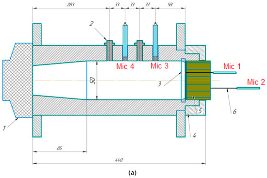
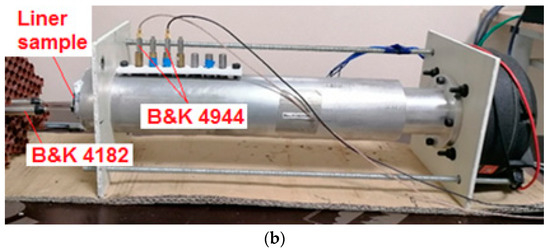 Figure 1. Impedance measurements by the transfer function method and Dean’s method: (a) diagram: Mic 1, Mic 2—microphones for Dean’s method; Mic 3, Mic 4—microphones for transfer function method; 1. acoustic driver; 2. plug; 3. supporting ring; 4. sample holder; 5. liner sample; 6. probe microphones; (b) photo.
 - Dean’s method [3], in which probe microphones are inserted into the front plate and bottom of the liner sample (Mic 1 and Mic 2 in Figure 1a).
The measurements are performed synchronously.
Liner samples are measured in a normal incidence impedance tube with a duct diameter of 50 mm (Figure 1), making it possible to place seven complete cells in the liner sample and thereby obtain more representative data in the experiment than from impedance tubes with narrower ducts. However, in the conventional configuration of the normal incidence impedance tube [31], the liner sample is mounted inside a sample holder (a thick-walled tube, which is an extension of the impedance tube) and rigidly fixed with a piston. This configuration does not enable the impedance measurement by Dean’s method, as the probe microphones cannot be properly installed into the sample. In this regard, for synchronous impedance measurements by the transfer function method and Dean’s method, a modified sample holder (pos. 4 in Figure 1a) is used, which is attached to the impedance tube. A liner sample is mounted into the holder such that part of the sample is located outside the holder, making it possible to insert thin, stiff probe tubes into the front plate and the bottom of the sample (pos. 6 in Figure 1a). The impedance measurements by the transfer function method are obtained with two Bruel & Kjaer 4944 microphones; measurements by Dean’s method are obtained with two Bruel & Kjaer 4182 probe microphones (Figure 1b). The 4182 microphones use 50-mm stiff probe tubes. All microphones were calibrated before liner sample measurements using a Bruel & Kjaer Pistonphone 4228 with appropriate adapters.
Under conditions of normal wave incidence, the impact on all cells of a liner sample is considered to be the same. However, our experience with Dean’s method demonstrates that, in some cases, the sound field in the central cell of the sample may differ from the field in the remaining cells. This differences results in a difference in impedance determined by Dean’s method from the sound pressure measurements in the center cell and in the side cells. In this regard, we install the probe microphones only in the side cells (Figure 2).
Figure 2.
3D model of the liner sample.
It is also important to note the design specifics of the liner samples. Each resonator has the same number of holes arranged in the same way, while there are no holes in other places of the sample. The outermost cells are not perforated so that the plots of impedance do not show additional peaks associated with the resonance of these small cells. To keep the volume of non-perforated cells inscribed in a 50 mm-diameter circle as small as possible, the edges of the cells are chosen to be 9 mm. The remaining geometric parameters of the tested samples are presented in Table 1. They are within the ranges of parameters from the empirical databases used in the impedance models described above. The geometry of each sample is selected so that its resonance frequency differs markedly that from other samples.

Table 1.
Geometric parameters of the acoustic liner samples.
Samples with this specific geometry are produced by 3D printing. The perforated plate and honeycomb are printed as a single unit, while the bottom of the sample is printed separately and glued to the sample. Holes 1 mm in diameter for stiff probe tubes are printed with the sample, and then they are drilled to a diameter of 1.2 mm (conventional mechanical drilling is used). Then, the stiff probe tubes with an outer diameter of 1.24 mm are inserted into the holes with an interference fit. This decision increases the positioning accuracy of the probes and facilitates their installation into the sample. The liner sample with installed probes is mounted into the sample holder with an interference fit and additional sealing.
The experiments are carried out at 100, 110, 120, 130, 135, 140, 145 and 150 dB on the faces of the samples. At relatively low SPLs, the impedance changes little; therefore, in the range of 100–130 dB, a step of 10 dB is chosen. At high SPLs, small changes in SPL already notably affect the impedance, so the measurements are obtained in 5-dB steps. For each given SPL, measurements are performed in the frequency range of 500–3500 Hz with a step of 100 Hz. The environmental conditions in the experiment are as follows: ambient pressure of 1000 hPa; ambient temperature of 26 °C; and ambient humidity of 13%.
The “white noise” excitation and “sine” excitation are used in the experiments. In the case of “white noise” excitation, the entire set of required frequencies is immediately realized, and the total SPL over frequencies is controlled on the face of the liner sample, so SPL selection can be carried out fairly quickly by setting the voltage on an acoustic driver in manual mode. In the case of “sine” excitation, the situation becomes more complicated because measurements for each frequency must be obtained at an individual voltage on the acoustic driver. This requirement occurs for the following reasons:
- The wavelength changes as the frequency changes, so SPL changes along an impedance tube and consequently on the face of a sample;
- The absorption of sound energy changes with frequency (especially in a region of resonance frequencies); therefore, the SPL on the face of a sample changes too; and
- The characteristics of the acoustic driver change in frequency (for example, to maintain a required SPL at low frequencies of sound generation, less voltage should be applied to the acoustic driver than at high frequencies).
Obviously, in this situation, automation of the measurements is required because the selection of the acoustic driver voltage in manual mode is extremely laborious. For this purpose, code was written in MATLAB. First, the problem of controlling measurements from MATLAB was solved: since the sound generation and registration of signals are driven through Bruel & Kjaer PULSE Labshop software, the MATLAB code gains access to the methods and properties of the PULSE Labshop objects. In particular, the MATLAB code:
- Transfers the required voltage value and the sound generation frequency to PULSE Labshop;
- Starts the generation of the sound signal and synchronous fft-analysis of the signals registered on the microphones; and
- Reads from the PULSE Labshop the auto- and cross-spectra obtained in the fft-analysis.
The voltage selection is implemented through the MATLAB optimization function fminbnd, searching for the minimum of the objective function, which is the modulus of the difference between the target and the actual SPL measured with a probe microphone on the face of the liner sample. It is important to note that an SPL difference of, for example, 0.3 dB from the target value will not notably affect the change in impedance. However, the fminbnd function searches for a unimodal minimum using a golden section search and parabolic interpolation, where a procedure stops if the width of the interval becomes less than the given tolerance or if the given number of iterations is attained. Both of these parameters cannot be perfectly tuned, as they may differ for each liner sample depending on the frequency and SPL considered. As a result, it is necessary to set the number of iterations with a safety margin, despite in some cases the SPL deviation range of 0.3 dB being able to be attained already in the second or third iteration, but the iterations continue to run until the specified value of or is attained. Considering that a new measurement is required to determine a new value of the objective function, and one measurement requires at least 10 s before the SPL ceases to notably change, the procedure for selecting the voltage at one particular frequency can take several minutes. Thus, to reduce the duration of the experiment, a condition was added to the fminbnd function to stop the optimization when the discrepancy between the target and actual SPL values attained is dB.
The flowchart of the algorithm developed for measurements is shown in Figure 3. Here, is the target value of SPL on microphone 1, dB; is the sound generation frequency in Hz; and are voltage search limits in V; is the termination tolerance on the residual in dB; is the termination tolerance on the width of the search interval in V; is the maximum number of iterations allowed; is the actual voltage of the acoustic driver in V; is the actual value of the SPL on the microphone 1 in dB; is the objective function; is the residual in dB; and is the iteration number.
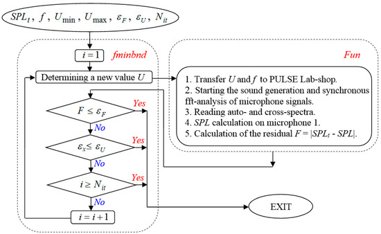
Figure 3.
Flowchart of the measurements on a normal incidence impedance tube with “sine” excitation.
Auto- and cross-spectra on microphones corresponding to the minimum residual are stored in a file for further calculation of the sample impedance by the transfer function method and Dean’s method.
4. Results of the Study
Due to the large volume of results, below are graphs of the normalized impedance only for SPLs on the face of a sample equal to 100, 130 and 150 dB. These SPLs are quite enough to represent the main trends in the behavior of the impedance: 100 dB—linear regime; 130 dB—the non-linearity of the impedance is not yet so strong; and 150 dB—deeply nonlinear regime.
Figure 4 and Figure 5 compare normalized impedance obtained by Dean’s method at 100 and 150 dB with “white noise” and “sine” excitation, respectively (the results of the transfer function method are not shown since all the conclusions drawn below are similar for them). First, we note that the reactance values are in good agreement with each other, both at low and at high SPLs. It can also be seen that, at 100 dB, the resistance levels at “white noise” and “sine” also agree well with each other. Thus, for acoustic liners used in ducts with SPLs corresponding to a linear regime, the impedance can be determined experimentally at “white noise”, which considerably reduces the labor of measurements due to the realization of the entire set of required frequencies in one sound generation.
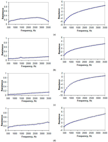
Figure 4.
Normalized impedance obtained by Dean’s method at 100 dB: (a) Sample 1; (b) Sample 2; (c) Sample 3; (d) Sample 4;  “white noise” excitation;
  “sine” excitation.
“white noise” excitation; “sine” excitation.
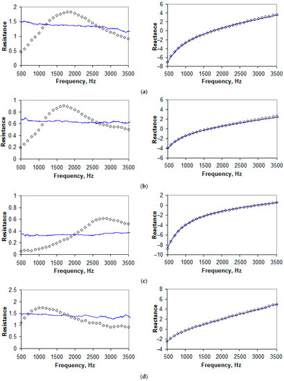
Figure 5.
Normalized impedance obtained by Dean’s method at 150 dB: (a) Sample 1; (b) Sample 2; (c) Sample 3; (d) Sample 4; “white noise” excitation; “sine” excitation.
“white noise” excitation; “sine” excitation.
At SPLs corresponding to a deeply nonlinear regime, the resistance at “white noise” and “sine” is unusual even in a qualitative sense. This effect is well known and is explained by the sound energy at “white noise” being distributed over all considered frequencies, so the SPL at each specific frequency is somewhat less than that at the total level. However, a semi-empirical theory is built on the assumption that all sound energy is concentrated at a single frequency, and “sine” excitation in the experiments is much better suited to this assumption than “white noise”. In this regard, to compare semi-empirical models across a wide range of SPLs, further plots are given for the experimental impedance values obtained with “sine” excitation.
In the plot of resistance values determined by Dean’s method for Sample 1 (Figure 4a), there is a strong drop after 3000 Hz. The result is probably caused by a slight distortion of one of the stiff probe tubes installed in Sample 1. This distortion can lead to an increase in the resistance of the tube channel at high frequencies. At the same time, a high SPL is capable of “overcoming” this resistance, and at 150 dB, such a drop is no longer registered (Figure 5a). When measuring the other samples, this distortion in the installation of the probe tubes is corrected.
The experimental reactance in Figure 4 shows that the resonance frequencies of the considered samples are in different regions of the frequency range: for Samples 1 and 2, in the region of 1600–1700 Hz; for Sample 3, in the region of 2800 Hz; and for Sample 4, in the region of 1000 Hz. This fact expands the variety of impedance behaviors and consequently allows us to perform a more complete assessment of the accuracy of describing the impedance by semi-empirical models for liners with different geometries.
The calculations by Models (1)–(4) were carried out using the empirical constants and dependencies presented in [16,17,21]. The discussion of the calculation results and their comparisons with experiments are carried out in the next section.
5. Discussion
Analyzing the formulas in Section 2, it can be noted that, although the considered semi-empirical theories are based on the works of Melling [11] and Guess [12], they differ in the values of the empirical constants and semi-empirical dependencies describing various physical effects. This difference occurs partly because the dependences and constants are obtained from measurements of samples with different designs under different conditions. Furthermore, there are differences in the methods for obtaining empirical data (numerical simulation, in-situ measurements, air blowing, etc.) and in the experimental rigs. In this regard, when calculating the impedance of a liner with a slightly different geometry than that considered in semi-empirical models, some discrepancy with the experimental impedance is observed. Obtaining semi-empirical dependences and constants for the new liner geometry requires long-term studies; therefore, a rational approach may be used for certain semi-empirical models that provide good agreement with the experiment in certain frequency ranges at given SPLs. The results of the calculations are further compared in this vein.
It is also important to note that the study reveals that all semi-empirical models demonstrate much better agreement with the experimental results determined by Dean’s method than by the transfer function method. This outcome can be explained by semi-empirical models being derived for a single resonator, and Dean’s method determines the impedance of only one cell, while the transfer function method determines the impedance of the entire face of the sample, as demonstrated in [32]. In this case, the open area ratio of a single resonator can differ from the liner sample containing an array of the resonators. However, the calculation carried out in the current study based on Models (1)–(4) for an open area ratio corresponding to the entire face of the sample yielded worse agreement with the experimental impedance determined by the transfer function method. For this reason, we discuss below only the agreement of semi-empirical models with the experimental impedance determined by Dean’s method.
Figure 6 shows that, at a low SPL, the resistance in the frequency range of 500–3500 Hz in the absence of grazing flow is best described by the Sobolev model and worst of all by the Eversman model. For Sample 2, which is not micro-perforated (t/d ≤ 1), the resistance calculated by the Goodrich model is also very close to the experiment (Figure 6b). The reactance at low SPLs for all samples is also best described by the Sobolev model. For Samples 1 and 4, the worst agreement for the reactance was obtained by the Eversman model and, for Sample 2, by the Goodrich model.
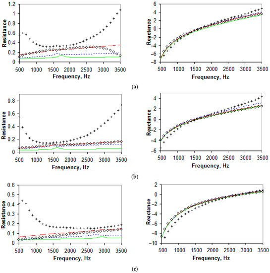
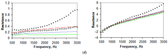
Figure 6.
Normalized impedance at 100 dB: (a) Sample 1; (b) Sample 2; (c) Sample 3; (d) Sample 4;  transfer function method; Dean’s method;
  Goodrich’s model;
  Sobolev’s model;
  Eversman’s model.
transfer function method; Dean’s method; Goodrich’s model; Sobolev’s model; Eversman’s model.
In the case of not strong nonlinearity (Figure 7), different impedance models demonstrate the best agreement of resistance with the experiment depending on the frequency range. For example, in the region of resonance frequencies for Sample 1, the Goodrich model turned out to be closest to the experiment, and for Samples 2, 3 and 4, the Eversman model was best. Additionally, the Goodrich model has good agreement: for Sample 2, in the range of 500–1500 Hz; for Sample 3, in the range of 500–2000 Hz; and for Sample 3, in the range of 1100–2700 Hz. The Sobolev model demonstrates the best agreement of reactance with the experiment for all samples.
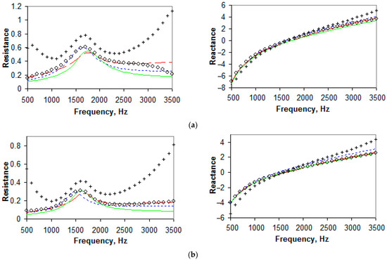
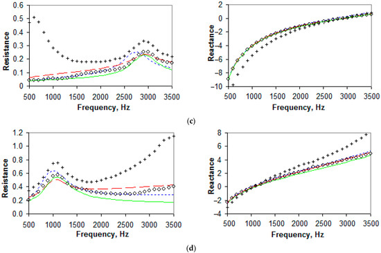
Figure 7.
Normalized impedance at 130 dB: (a) Sample 1; (b) Sample 2; (c) Sample 3; (d) Sample 4; transfer function method; Dean’s method; Goodrich’s model; Sobolev’s model; Eversman’s model.
transfer function method; Dean’s method; Goodrich’s model; Sobolev’s model; Eversman’s model.
At a high SPL (Figure 8), the resistance and reactance in the frequency range of 500–3500 Hz for Samples 1 and 4 are best described by the Goodrich model and worst of all by the Sobolev model. For Samples 2 and 3, the Eversman model best describes the impedance in the frequency range of 500–2500 Hz. The Sobolev model turned out to be close in resistance to that from the experiment only for Sample 3 in the frequency range of 3000–3500 Hz.
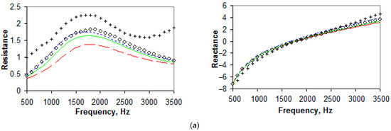
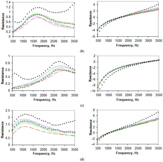
Figure 8.
Normalized impedance at 150 dB: (a) Sample 1; (b) Sample 2; (c) Sample 3; (d) Sample 4; transfer function method; Dean’s method; Goodrich’s model; Sobolev’s model; Eversman’s model.
transfer function method; Dean’s method; Goodrich’s model; Sobolev’s model; Eversman’s model.
Near zero reactance, the best agreement with the experiment for all cases was noted for the Sobolev model. This finding can be explained by the Sobolev model using a more developed semi-empirical dependence for the end correction.
Note also that we did not consider here such a strong effect for impedance as the in-duct grazing flow (impedance calculations were performed with a mean Mach number of the in-duct grazing flow equal to 0). This problem has been the subject of much work considering the construction of the experimental rigs called the “grazing flow impedance tube” or “grazing flow impedance duct”, measurement methods (especially regarding the flow velocity profile) and impedance reduction methods [4,5]. Research on the “grazing flow impedance tube” for comparison of semi-empirical impedance models of locally-reacting acoustic liners, which we intend to carry out in the future studies, is a more time-consuming task, although measurements on a normal incidence impedance tube can also be very laborious if, for example, the method using a standing wave ratio [1] is applied.
6. Conclusions
As a result of the conducted study, it can be concluded that:
- If the validation of a semi-empirical impedance model of locally reacting liner is carried out by measurements on a normal incidence impedance tube, then it is better to use “sine” excitation and Dean’s method because they better correspond to the conditions used when deriving an impedance model;
- At a low SPL on the face of a liner sample, the impedance is better described by the Sobolev model;
- At a high SPL on the face of a liner sample, the impedance is well described by the Goodrich or Eversman model (depending on the geometry of a sample); and
- In the presence of a variable SPL on the face of a liner sample (e.g., grazing incidence), it is obviously necessary to use several different impedance models, each in certain sections of the liner, ensuring a smooth change in the impedance when transferring from one model to another.
Thus, among the considered semi-empirical models, there is no model that equally well describes impedance under all conditions due to the complexity of the problems to be solved when developing the model.
Author Contributions
Conceptualization, V.P., A.K., and I.K.; methodology, V.P., A.K., and I.K.; software, V.P. and A.K.; validation, I.K. and O.K.; formal analysis, V.P., A.K., and I.K.; investigation, V.P., A.K., I.K., and O.K.; resources, V.P.; data curation, V.P.; writing—original draft preparation, V.P., A.K., I.K., and O.K.; writing—review and editing, V.P. and A.K.; visualization, O.K.; supervision, V.P.; project administration, V.P.; funding acquisition, V.P. All authors have read and agreed to the published version of the manuscript.
Funding
This study was funded by a grant from the Perm Region and Russian Science Foundation, grant number 22-22-20087.
Data Availability Statement
Not applicable.
Conflicts of Interest
The authors declare no conflict of interest.
References
- ISO 10534-1; Acoustics—Determination of Sound Absorption Coefficient and Impedance in Impedance Tubes. Part 1: Method Using Standing Wave Ratio. ISO: Geneva, Switzerland, 1996.
- ISO 10534-2; Acoustics—Determination of Sound Absorption Coefficient and Impedance in Impedances Tubes. Part 2: Transfer-Function Method. ISO: Geneva, Switzerland, 1996.
- Dean, P.D. An in-situ method of wall acoustic impedance measurement in flow duct. J. Sound Vib. 1974, 34, 97–130. [Google Scholar] [CrossRef]
- Watson, W.R.; Jones, M.G. A comparative study of four impedance eduction methodologies using several test liners. In Proceedings of the 19th AIAA/CEAS Aeroacoustics Conference, Berlin, Germany, 27–29 May 2013. [Google Scholar]
- Ostrikov, N.N.; Yakovets, M.A.; Ipatov, M.S. Confirmation of an analytical model of the sound propagation in a rectangular duct in the presence of impedance transitions and development of an impedance eduction method based on it. Acoust. Phys. 2020, 66, 105–122. [Google Scholar] [CrossRef]
- Tam, C.K.W.; Kurbatskii, K.A. A numerical and experimental investigation of the dissipation mechanisms of resonant acoustic liners. J. Sound Vib. 2001, 245, 545–557. [Google Scholar] [CrossRef]
- Roche, J.M.; Leylekian, L.; Delattre, G.; Vuillot, F. Aircraft fan noise absorption: DNS of the acoustic dissipation of resonant liners. In Proceedings of the 15th AIAA/CEAS Aeroacoustics Conference (30th AIAA Aeroacoustics Conference), Miami, FL, USA, 11–13 May 2009. [Google Scholar]
- Zhang, Q.; Bodony, D.J. Impedance predictions of 3D honeycomb liner with circular apertures by DNS. In Proceedings of the 17th AIAA/CEAS Aeroacoustics Conference (32nd AIAA Aeroacoustics Conference), Portland, OR, USA, 5–8 June 2009. [Google Scholar]
- Palchikovskiy, V.; Khramtsov, I.; Kustov, O. On the influence of certain geometric characteristics of the resonator on the impedance determined by the Dean’s method. Acoustics 2022, 4, 382–393. [Google Scholar] [CrossRef]
- Ou, Y.; Zhao, Y. Prediction of the absorption characteristics of non-uniform acoustic absorbers with grazing flow. Appl. Sci. 2023, 13, 2256. [Google Scholar] [CrossRef]
- Melling, T.H. The acoustic impendance of perforates at medium and high sound pressure levels. J. Sound Vib. 1973, 21, 1–65. [Google Scholar] [CrossRef]
- Guess, A.W. Calculation of perforated plate liner parameters from specified acoustic resistance and reactance. J. Sound Vib. 1975, 40, 119–137. [Google Scholar] [CrossRef]
- Kooi, J.W.; Sarin, S.L. An experimental study of the acoustic impedance of Helmholtz resonator arrays under a turbulent boundary layer. In Proceedings of the 7th Aeroacoustics Conference, Palo Alto, CA, USA, 5–7 October 1981. [Google Scholar]
- Motsinger, R.E.; Kraft, R.E. Design and performance of duct acoustic treatment. In Aeroacoustics of Flight Vehicles. Theory and Practice. Volume 2: Noise Control; Hubbard, H.H., Ed.; NASA Langley Research Center: Hampton, VA, USA, 1991; pp. 165–206. [Google Scholar]
- Hersh, A.S.; Walker, B.E.; Celano, J.W. Helmholtz resonator impedance model, Part 1: Nonlinear behavior. AIAA J. 2003, 41, 795–808. [Google Scholar] [CrossRef]
- Yu, J.; Ruiz, M.; Kwan, H.W. Validation of Goodrich perforate liner impedance model using NASA Langley test data. In Proceedings of the 14th AIAA/CEAS Aeroacoustics Conference (29th AIAA Aeroacoustics Conference), Vancouver, BC, Canada, 5–7 May 2008. [Google Scholar]
- Sobolev, A.F. A semiempirical theory of a one-layer cellular sound-absorbing lining with a perforated face panel. Acoust. Phys. 2007, 53, 762–771. [Google Scholar] [CrossRef]
- Murray, P.B.; Astley, R.J. Development of a single degree of freedom perforate impedance model under grazing flow and high SPL. In Proceedings of the 18th AIAA/CEAS Aeroacoustics Conference (33rd AIAA Aeroacoustics Conference), Colorado Springs, CO, USA, 4–6 May 2012. [Google Scholar]
- Murray, P.B.; Donnan, C.; Richter, C.; Astley, J. Development of a single degree of freedom microperforate impedance model under grazing flow and high SPL. In Proceedings of the 22nd AIAA/CEAS Aeroacoustics Conference, Lyon, France, 30 May–1 June 2016. [Google Scholar]
- Rienstra, S.W.; Singh, D.K. Nonlinear asymptotic impedance model for a Helmholtz resonator of finite depth. AIAA J. 2018, 56, 1792–1802. [Google Scholar] [CrossRef]
- Eversman, W.; Drouin, M.; Locke, J.; McCartney, J. Impedance models for single and two degree of freedom linings and correlation with grazing flow duct testing. Int. J. Aeroacoustics 2021, 20, 497–529. [Google Scholar] [CrossRef]
- Stinson, M.R.; Shaw, E.A. Acoustic impedance of small, circular orifices in thin plates. J. Acoust. Soc. Am. 1985, 77, 2039–2042. [Google Scholar] [CrossRef]
- Elnady, T.; Boden, H. On semi-empirical liner impedance modeling with grazing flow. In Proceedings of the 9th AIAA/CEAS Aeroacoustics Conference and Exhibit, Hilton Head, SC, USA, 12–14 May 2003. [Google Scholar]
- Komkin, A.; Bykov, A.; Saulkina, O. Evaluation of the oscillation velocity in the neck of the Helmholtz resonator in nonlinear regimes. Acoustics 2022, 4, 564–573. [Google Scholar] [CrossRef]
- Kraft, R.E.; Yu, J.; Kwan, H.W. Acoustic treatment impedance models for high frequencies. In Proceedings of the 3rd AIAA/CEAS Aeroacoustics Conference, Atlanta, GA, USA, 12–14 May 1997. [Google Scholar]
- Yu, J.; Kwan, H.W.; Chiou, S. Microperforate plate acoustic property evaluation. In Proceedings of the 5th AIAA/CEAS Aeroacoustics Conference and Exhibit, Bellevue, WA, USA, 10–12 May 1999. [Google Scholar]
- Fok, V.A. Theoretical study of the conductance of a circular hole in a partition across a tube. Proc. USSR Acad. Sci. 1941, 31, 875–882. [Google Scholar]
- Parrott, T.L.; Jones, M.G. Chapter 6—Uncertainty in acoustic liner impedance measurement and prediction. In Assessment of NASA’s Aircraft Noise Prediction Capability; Dahl, M.H., Ed.; NASA Glenn Research Center: Cleveland, Ohio, USA, 2012; pp. 157–204. [Google Scholar]
- Schultz, T.; Liu, F.; Cattafesta, L.; Sheplak, M.; Jones, M. A comparison study of normal-incidence acoustic impedance measurementsof a perforate liner. In Proceedings of the 15th AIAA/CEAS Aeroacoustics Conference (30th AIAA Aeroacoustics Conference), Miami, FL, USA, 11–13 May 2009. [Google Scholar]
- Spillere, A.M.; Braga, D.S.; Seki, L.A.; Bonomo, L.A.; Cordioli, J.A.; Rocamora, B.M., Jr.; Greco, P.C., Jr.; dos Reis, D.C.; Coelho, E.L. Design of a single degree of freedom acoustic liner for a fan noise test rig. Int. J. Aeroacoustics 2021, 20, 708–736. [Google Scholar] [CrossRef]
- Palchikovskiy, V.V.; Kustov, O.Y.; Korin, I.A.; Cherepanov, I.E.; Khramtsov, I.V. Investigation of acoustic characteristics of liner samples in interferometers with different duct diameter. PNRPU Aerosp. Eng. Bull. 2017, 51, 62–73. [Google Scholar] [CrossRef]
- Khramtsov, I.; Kustov, O.; Palchikovskiy, V.; Ershov, V. Investigation of the reason for the difference in the acoustic liner impedance determined by the transfer function method and Dean’s method. Akustika 2021, 39, 224–229. [Google Scholar] [CrossRef]


Disclaimer/Publisher’s Note: The statements, opinions and data contained in all publications are solely those of the individual author(s) and contributor(s) and not of MDPI and/or the editor(s). MDPI and/or the editor(s) disclaim responsibility for any injury to people or property resulting from any ideas, methods, instructions or products referred to in the content. |
© 2023 by the authors. Licensee MDPI, Basel, Switzerland. This article is an open access article distributed under the terms and conditions of the Creative Commons Attribution (CC BY) license (https://creativecommons.org/licenses/by/4.0/).