1. Introduction
Blind signal separation (BSS) has been of great interest for various practical applications, including image enhancement, speech enhancement, and biomedical signal processing [
1,
2,
3,
4,
5,
6,
7,
8]. This is attributed to the fact that BSS has the ability to separate sources from the observed mixtures without requiring source localization knowledge or array geometry information. Such flexibility has made BSS a popular technique in many applications.
In general, BSS techniques can be classified into the classes of higher order-based BSS and second order-based BSS. Higher order-based BSS requires assumption of the source density function. Second order-based BSS, on the other hand, requires assumption of the second order statistics of the source, such as non-stationarity or non-whiteness. In this paper, we concentrate on second order-based BSS.
The second order-based BSS for convolutive mixtures with fixed step size has previously been investigated in [
4]. In [
9], a steepest descent algorithm with an optimum step size procedure was proposed for the second order gradient-based BSS to improve the convergence. In [
7,
10], a conjugate gradient algorithm was developed for the BSS problem in which a transformation is employed to convert the constrained optimization problem with complex unmixing matrices into an unconstrained optimization problem. An accelerated gradient method with optimal step size was proposed for solving the problem in [
8]. The algorithm was combined with the kurtosis measure and single speech enhancement technique to further reduce the background noise in the speech-dominant outputs.
In this paper, we propose improving the convergence rate of the accelerated gradient BSS algorithm further by incorporating the conjugate gradient descent into the accelerated algorithm. The search direction for each iteration is obtained by utilizing both the accelerated gradient descent direction at the current iteration and the direction obtained from the previous iteration. The idea of an accelerated conjugate gradient algorithm has previously been applied for MR Imaging reconstruction in [
11,
12]. The image processing problem uses sparsity in the cost function according to [
11]. Here, the audio separation is applied to short-time Fourier transform (STFT) signals over different time lags, and correlation matrices are formed for each frequency and time lag. Then, we use the non-stationarity of the speech sources as a criterion by diagonalizing multiple correlation matrices over a range of different time lags. As such, the key observation is the non-stationarity of the speech sources. Thus, the problem formulation for the speech separation problem is very different from the image processing problem; however, we have found that the accelerated conjugate gradient update can be used for both problems. In addition, a linear search method is employed to obtain the optimal step size for each iteration. This results in an accelerated conjugate gradient algorithm with optimal step size.
In addition, we calculate the optimal step size for each iteration in order to improve the convergence of the accelerated conjugate gradient algorithm. Simulation results based on data from a simulated room environment and real data from a recording environment show that the proposed algorithm converges faster than the accelerated algorithm and the steepest descent algorithm while requiring approximately the same computational complexity per iteration. This results in a lower total computational complexity for convergence of the accelerated conjugate gradient algorithm, as the proposed algorithm requires fewer iterations for convergence. In addition, the proposed system can simultaneously separate sources and suppress noise in reverberant environments, resulting in improved signal-to-interference and signal-to-noise ratios compared to existing methods.
The rest of this paper is organized as follows. The second order BSS is formulated in
Section 2. In
Section 3, the accelerated conjugate gradient algorithm is developed. Simulation results are provided in
Section 4, and
Section 5 contains the conclusions.
2. Second Order Blind Signal Separation
Consider the model used in [
4] for a convolutive mixture of
N sources in which the received signal vector with
L microphones is
and where
t is the sampled time index. The received signal vector is passed through
unmixing matrices
, where
Q is the length of the unmixing filters, producing an output signal vector
:
The objective is to estimate the unmixing matrices
to recover the sources up to an arbitrary scaling and permutation [
4]. The exact number of sources is usually unknown, and is assumed to be the same as the number of microphones, i.e.,
. The received signal is processed in block BSS in the frequency domain. The signal is divided into
M blocks, and the correlation matrix
,
for each frequency
is calculated [
9], where
denotes the frequency set.
We denote by
the set consisting of all the frequency domain unmixing matrices
. The problem is to estimate
that jointly decorrelates
M correlation matrices
. This problem can be formulated as minimizing the following weighted cost over the frequencies
,
where
and
is the Frobenius norm. Here, offdiag{·} denotes the matrix which the same as {·} for elements outside the diagonal and zeros for elements along the diagonal. The weighting function
is obtained from the correlation matrix
as
Additional constraints on the unmixing matrices are included to avoid a zero solution, where the diagonal elements of the matrix
are restricted to being one for all
k, i.e.,
for all
. The minimization of the weighted cost function in (
2) can lead to an arbitrary permutation of the frequency bins. A method to overcome this problem is to constrain the corresponding time domain unmixing weight
to length
D. This effectively requires zero coefficients for time domain elements greater than
D, which restricts the solutions to being continuous or smooth in the frequency domain [
4]. As such, the optimization problem to obtain the unmixing weighting matrix can be formulated as follows:
3. Accelerated Conjugate Gradient Algorithm
In [
8], the accelerated gradient algorithm was developed to solve problem (
5). Here, we propose the combination of the accelerated gradient algorithm and the conjugate gradient algorithm to further improve the convergence of the optimization problem in (
5). This results in an accelerated conjugate gradient algorithm with a step size optimized for each iteration. As problem (
5) restricts the elements along the diagonal of matrix
for all
w to 1, we only need to update the coefficients for the off-diagonal elements. For each iteration
, the descent search direction is calculated as
where ∇ denotes the gradient. This direction is then transformed into the time domain and the coefficients are truncated to a length
D. The constrained time domain search direction is transformed back into the frequency domain to obtain the direction
.
For each iteration
k of the accelerated gradient algorithm [
8], instead of using the descent direction at
we use the descent direction at the point
, which is a combination of the unmixing matrices
and
at the
k and
k − 1 iterations, respectively:
This provides an improvement in the convergence of the accelerated algorithm, as it takes into consideration the unmixing matrix at the previous iterations [
13,
14,
15]. The descent direction at
is obtained, resulting in
. Similar to
, this direction is then transformed into the time domain and the coefficients are truncated to a length
D. The constrained time domain search direction is transformed back into the frequency domain, resulting in the direction
.
With the accelerated conjugate gradient algorithm [
11], instead of using the gradient direction
from
, the conjugate gradient direction is set based on the gradient direction and the previous searched direction. We denote by
the search direction in the
direction. The search direction
at the
iteration is obtained from
and
as
where
is the step size, which is defined as in [
16,
17]. One possible choice for
is
where
denotes the
norm. The combination of the current search direction and the previous direction allows the algorithm to converge faster to the optimal solution compared to the accelerated algorithm.
For each iteration, the step size
is searched in the direction
as
The unmixing weight matrices are updated according to
The proposed algorithm can be summarized as follows:
Procedure 1: Accelerated conjugate gradient algorithm for BSS
For each iteration
k, the problem in (
10) becomes finding the optimal step size
that minimizes the objective function
. We now employ an efficient procedure for searching the optimum step size for each iteration
k. The search for
can be viewed as a one-dimensional optimization problem with respect to
. Thus, a line search using a golden search algorithm is employed to obtain the optimal step size. The search for the optimum step size can be described as follows.
Procedure 2: Search for an optimum step size
that minimizes the cost function (
10).
Step 1: Initialize a step size , a constant , and an accuracy level . Set , , and .
Step 2: Obtain the cost functions and . If , then reduce the initial step size by setting . Let and proceed to the beginning of Step 2. Otherwise, and continue to Step 3.
Step 3: Increase s by setting and let . Calculate the cost function . If , then set , and return to the beginning of Step 3. Otherwise, proceed to Step 4.
Step 4: We now have three points,
,
, and
, satisfying
Thus, there exists a local minimum in the interval
. As such, a parabola is fitted among three points
,
, and
. The minimum
a of this parabola in the interval
can be calculated using the parabola approximation [
7]. Update
; stop the procedure if
is small enough and output the optimal step size.
The advantage of Procedure 2 is that it is relatively simple. In addition, by combining parabolic interpolation with a step size search, the optimum step size can be found with just a few calculations of the cost function.
4. Design Examples
The proposed speech enhancement scheme is evaluated in a simulated room environment with a fast-ISM room simulator and in a real car recording environment. The performance measures for the source outputs are obtained by assuming the access of the source, interference, and noise separately. Here, fourth-order kurtosis is employed to determine the two outputs with dominant speech levels [
10]. A high value of kurtosis indicates that the distribution tends towards supergaussian. Because speech signals follow a Laplacian distribution, they belongs to the supergaussian case. For a case with speech sources, interference, and noise, the dominant speech outputs are determined as the ones corresponding to the highest kurtosis.
As such, fourth-order kurtosis is employed to determine the two most dominant speech output. For each output, the source with the highest power is viewed as the main source, while the other is viewed as the interference. Hence, for each output we denote
and
as the power spectral density (PSD) of the source, interference, and noise, respectively. The performance measure of each output is quantified in terms of a signal to interference ratio and signal to noise ratio, defined as
We first consider the case with a simulated room environment.
4.1. Case 1: Simulated Room Environment
We consider the case of a simulated room environment and a linear array; the room has dimensions
m
3 with a sampling rate
Hz (see
Figure 1). The inter-element distance for the microphone array is 0.04 m. We have three microphones at the
positions
,
, and
, respectively. The speech signal is from the TIMIT library and the noise is from the NOISEX-92 library. The signal-to-interference ratio (SIR) is 0 dB, while the signal-to-noise ratio (SNR) is 0 dB and 10 dB. The length of the data is 8 seconds. The outputs are obtained using a fast-ISM room simulator [
18] with reverberation time
s.
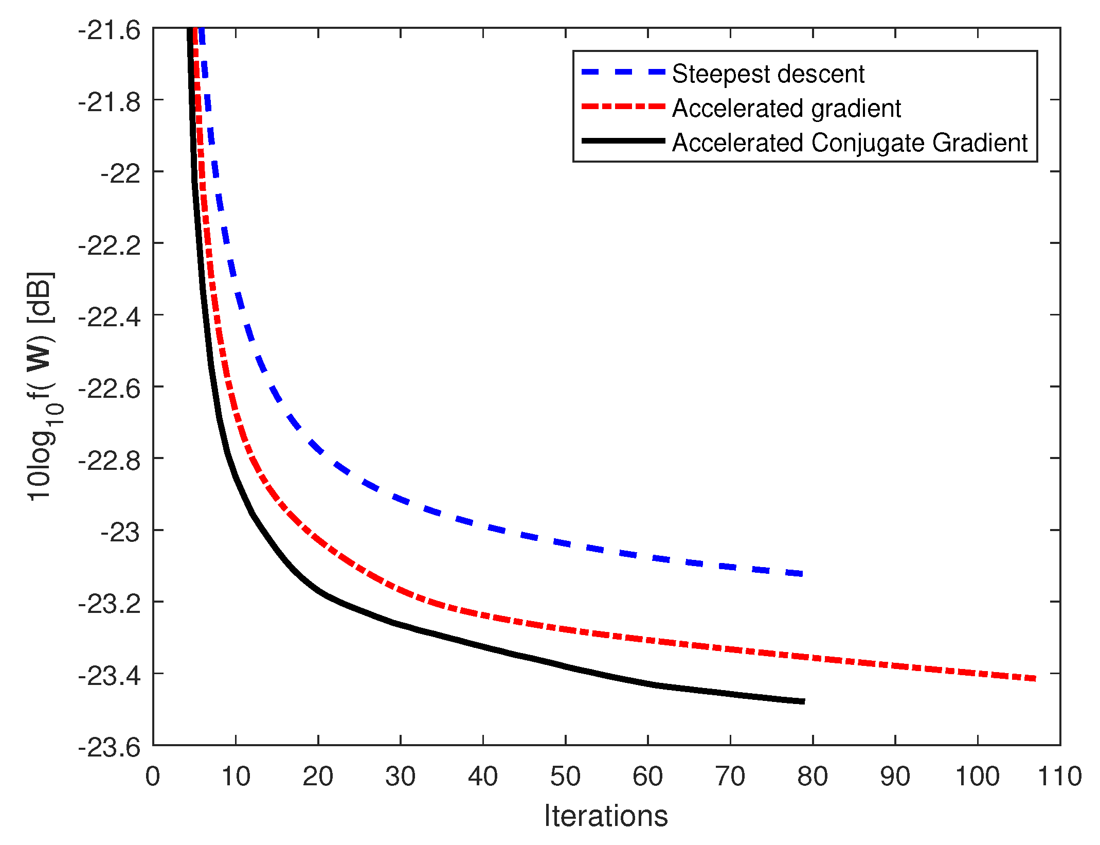
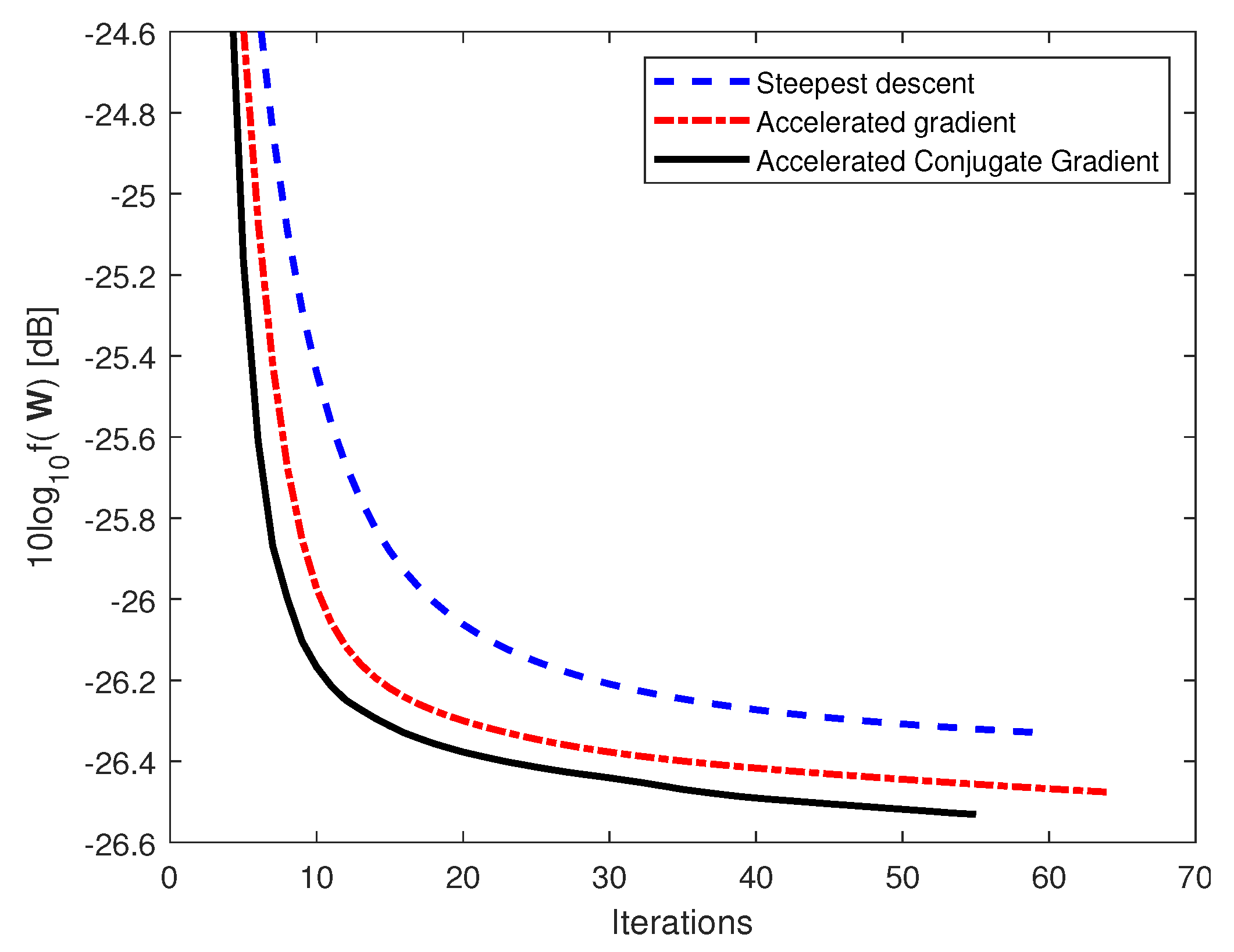
Figure 2 and
Figure 3 show the convergence for (i) the steepest descent, (ii) the accelerated gradient, and (iii) the accelerated conjugate gradient algorithms for the case with 0 dB and 10 dB SNR, respectively. All algorithms have optimal step size in each iteration and converge with
in (
13); moreover, we set the constant
as
and allow the unmixing weight matrices
to have a cost function up to 10% larger than the cost of the unmixing weight matrices
.
It can be seen from the figures that the accelerated conjugate gradient converges faster than the accelerated gradient and steepest descent algorithms for both SNR = 0 dB and 10 dB with a smaller objective function. In particular, for the case with SNR = 0 dB, the accelerated conjugate gradient requires 79 iterations for convergence with a smaller objective function, while the accelerated gradient requires 109 iterations for convergence.
Table 1 and
Table 2 show the SIR and SNR for the two dominant speech outputs for the three methods with the SNR = 0 dB and 10 dB, respectively. For each output, one speech is viewed as the source while the other is viewed as the interference. It can be seen from the tables that the accelerated conjugate gradient has improved performance over the other two methods.
For the case with 10 dB SNR, the accelerated conjugate gradient method has an improvement of 3.12 dB SIR over the steepest descent method and 0.75 dB SIR over the accelerated gradient method for the first output. For the second output, the accelerated conjugate gradient method has an improvement of 5.67 dB SIR over the steepest descent method and 1.60 dB SIR over the accelerated gradient method. Similar improvements of the accelerated conjugate gradient method over other existing methods can be seen with the SNR measure.
4.2. Case 2: Real Car Recording Data
We now consider a second case with recording data from a real car. Evaluations are performed for a double-talk situation in a real car hands-free environment for a Toyota Landcruiser 4WD driven on sealed roads at a speed of 60 km/h. A linear array with 40 mm spacing was mounted on the dashboard in front of the passenger seat. Data were gathered on a multichannel DAT-recorder with a sampling rate of 16 kHz. The main speech source is a male speaker in the front seat, while the interference is the female speaker in another seat. The male and female speech sources have the same power and operate at the same time, resulting in an SIR of 0 dB. The values of and are the same as in Case 1.
First, we focus on the convergence comparison between the accelerated conjugate gradient, the accelerated gradient method, and the steepest descent method.
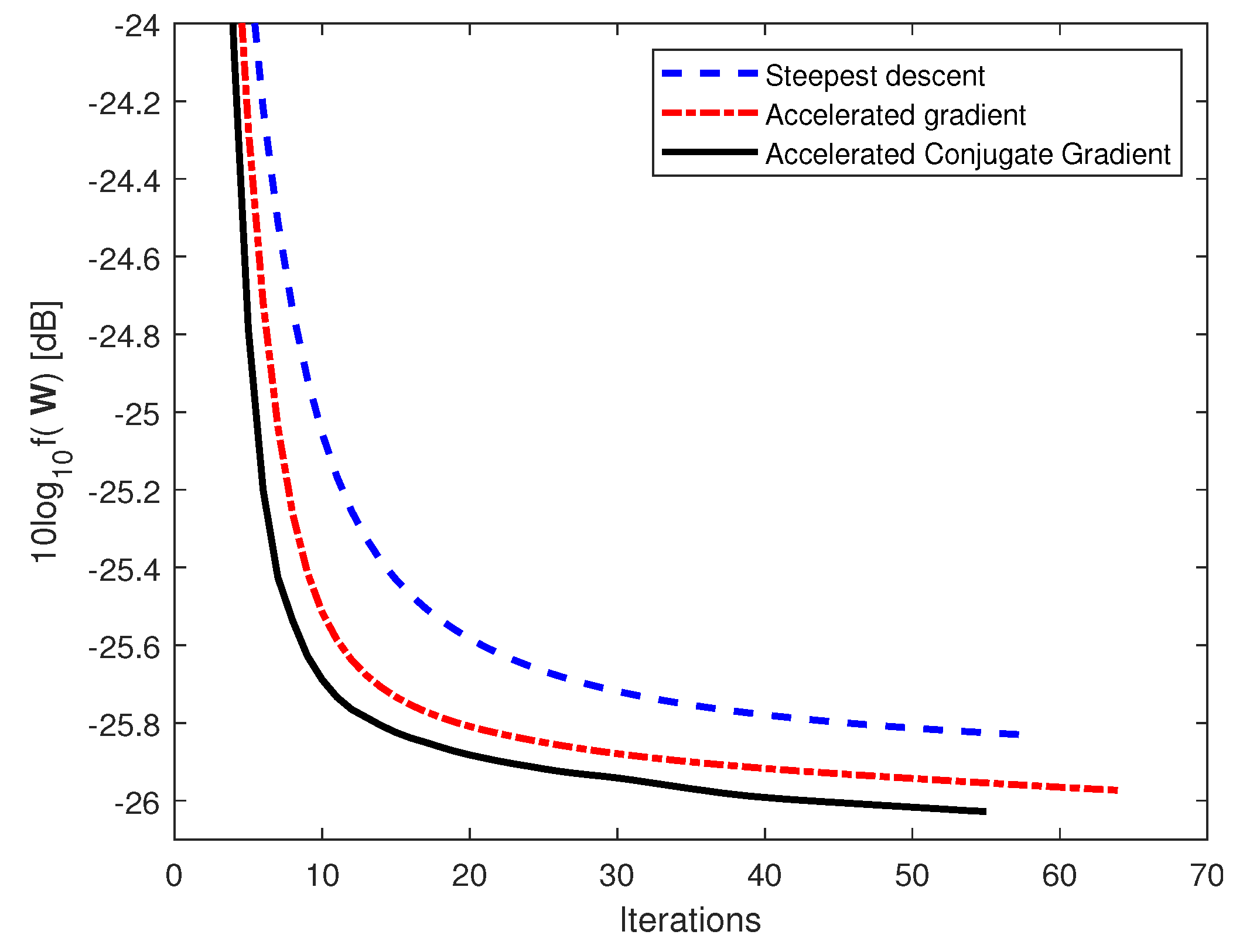
Figure 4 and
Figure 5 compare the convergence rates for the case with three microphones and SNR = 0 dB and 10 dB, respectively. It can be seen from both figures that the accelerated conjugate gradient with an optimal step size converges faster than the steepest descent and the accelerated gradient with optimal step size, with a lower objective function.
Table 3 and
Table 4 show the SIR and SNR measures for the two speech dominant outputs with SNR = 0 dB and 10 dB, respectively. The outputs from the accelerated conjugate gradient method have higher SIR and SNR when compared with the other two methods. In particular, for 0 dB input SNR, the first output for the accelerated conjugate gradient method achieves an improvement of 1.50 dB for SIR and 2.00 dB for SNR over the accelerated gradient method. In addition, the method achieves an improvement of 2.73 dB for SIR and 3.12 dB for SNR over the steepest descent method. For the second output, the accelerated conjugate gradient method achieves a 2.52 dB improvement for SIR and 4.08 dB for SNR over the accelerated gradient method. In addition, the method achieves an improvement of 2.66 dB for SIR and 5.36 dB for SNR over the steepest descent method.


