Temporal Howling Detector for Speech Reinforcement Systems

Abstract

In this paper, we address the problem of howling detection in speech reinforcement system applications for utilization in howling control mechanisms. A general speech reinforcement system acquires speech from a speaker’s microphone, and delivers a reinforced speech to other listeners in the same room, or another room, through loudspeakers. The amount of gain that can be applied to the acquired speech in the closed-loop system is constrained by electro-acoustic coupling in the system, manifested in howling noises appearing as a result of acoustic feedback. A howling detection algorithm aims to early detect frequency-howls in the system, before the human ear notices. The proposed algorithm includes two cascaded stages: Soft Howling Detection and Howling False-Alarm Detection. The Soft Howling Detection is based on the temporal magnitude-slope-deviation measure, identifying potential candidate frequency-howls. Inspired by the temporal approach, the Howling False-Alarm Detection stage considers the understanding of speech-signal frequency components’ magnitude behavior under different levels of acoustic feedback. A comprehensive howling detection performance evaluation process is designed, examining the proposed algorithm in terms of detection accuracy and the time it takes for detection, under a devised set of howling scenarios. The performance improvement of the proposed algorithm, with respect to a plain magnitude-slope-deviation-based method, is demonstrated by showing faster detection response times over a set of howling change-rate configurations. The two-staged proposed algorithm also provides a significant recall improvement, while improving the precision decrease via the Howling False-Alarm Detection stage.

1. Introduction

Speech reinforcement (SR) applications, whether in-room communication systems or remote audio teleconference systems, usually encompass an inherited level of acoustic feedback due to reverberation within the end-users’ locations. Such SR systems include public announcement (PA) systems, live shows, in-car communications, in-room and remote conference calls, and online video calls. SR systems consist of microphones, which aim to acquire each speaker’s direct (and least reverberant) speech, and loudspeakers that amplify the received speech signals and play them—back into the room or to the rooms of the end-users (assuming no earphones). Unfortunately, when the amplification gain rises, or the microphone is placed close to the loudspeaker, the level of acoustic feedback may become excessively high, i.e., electro-acoustic coupling, manifesting as grating howling noises. Namely, the acoustic echo from the loudspeaker might reach the speaker’s microphone due to reverberation, i.e., reflections of sound waves inside the room [1].

A room’s reverberation time (T₆₀) is dependent on the structure of the room, i.e., room dimensions, the materials of the walls, and its interior, where all of these affect the time taken for the sound signal to decay [2,3,4,5]. The room’s reverberation characteristics, together with the loudspeaker and microphone positions in the room, determine the sound waves’ direct path and reflections. These loudspeaker-enclosure-microphone (LEM) paths characterize the channel of the echo signal and directly affect the acoustic feedback in the room, which at some level of amplification gain might trigger electro-acoustic coupling and instability within the SR system, evoking howling at resonance frequencies of the system’s closed-loop transfer function (TF) [6,7,8]. The attainable gain of the loudspeakers is thus limited by a maximum stable gain (MSG) of the SR system [9]. However, the amplification gain is only limited around the howling frequencies. When a clean speech signal arrives at the microphone of a closed-loop SR system, assuming no thermal noise, only speech harmonics close to the poles of the TF can evoke howling. Therefore, evoked frequency-howls can be instinctively suppressed by changing the system’s TF, i.e., by reducing the amplification gain or altering the LEM paths. After that, it is possible to return the SR system to its initially configured state.

Two approaches are commonly used to tackle the howling problem in SR systems. To prevent electro-acoustic coupling, an acoustic echo canceller (AEC) is often used, both in hearing aids and in hands-free communication. AECs aim to cancel the echo signal from the loudspeaker by adaptively identifying the room-impulse-response (RIR) of the LEM paths and subtracting the estimated echo signal [1,3,10,11,12,13,14,15,16,17]. Another common (complementary) approach for acoustic feedback control is the use of notch-filter-based howling suppression (NHS) techniques, a private case of howling control mechanisms that aim at stabilizing the SR system by handling the appearance of frequency-howls (rather than preventing it) [12,13]. This approach consists of a howling detection algorithm and a notch filter design method, as in [7,18,19]. The state-of-the-art howling detection features are the PTPR (Peak-to-Threshold Power Ratio), PAPR (Peak-to-Average Power Ratio), PNPR (Peak-to-Neighboring Power Ratio), PHPR (Peak-to-Harmonic Power Ratio), IPMP (Interframe Peak Magnitude Persistence), and the IMSD (Interframe Magnitude Slope Deviation), as reviewed in [6,20]. The temporal IMSD feature evaluates the magnitude-increase of a frequency component as a function of time, by measuring the logarithmic magnitude’s frame-wise slope variation. Accordingly, Green et al. proposed the computationally efficient ‘summing’ method for assessing the MSD of frequency spectrum data [19]. Alternatively, a deep-learning-based approach for howling detection is proposed in [21], utilizing a convolutional recurrent neural network (CRNN)-based method for howling detection in real-time communication applications, which is robust to device-dependent howling features.

While AECs work very well in several cases, unobservable input speech signals acquired with the loudspeaker’s echo signal (double-talk), or changes in the room acoustics (RIR), may get the AEC out of tune and affect the sound quality and the stability of the SR system for the currently applied amplification gain [7,18]. Moreover, an AEC’s processing delay must be lower than the minimal propagation delay that may exist in the room (shortest LEM path) [22]. While NHS techniques may serve as a backup mechanism for handling the appearance of frequency-howls, they depend on an accurate and early howling detection algorithm. Furthermore, they may compromise speech quality in the case of over-filtering. Consequently, feedback control via howling detection remains a significant challenge for real-time applications. While the deep-learning-based approach was reported to achieve a high detection rate and a low false-alarm rate, its spectral image of 32 frames (1.28 s) suggests that howling would be noticed before being detected. Although the MSD measure is reported to be accurate [19], the temporal IMSD feature, on which it is based, is said to be extremely sensitive to the threshold choice [20]. Based on this, using the MSD measure alone might not be sufficient.

In this paper, a temporal howling detection algorithm, based on the MSD measure, is proposed for SR systems. The proposed algorithm aims to early detect frequency-howls in the system, before the human ear notices. Thus, laying the foundation for howling control mechanisms, and maintaining high-quality speech communication. The howling detection algorithm includes two cascaded stages: Soft Howling Detection and Howling False-Alarm Detection. The Soft Howling Detection is based on the temporal magnitude-slope-deviation measure, identifying potential candidate frequency-howls. As opposed to using a plain MSD-based detector, the Soft Howling Detection stage is designed to be less strict, detecting as many potential candidate frequency-howls as possible. Therefore, the detection process is immediate, identifying suspected feedback howls across all frequency bins. As the majority of howling false alarms can be attributed to frequency components of speech harmonics, the proposed solution aims to authenticate each suspected frequency-howl with regard to the signal behavior before detection. Inspired by the temporal approach, the Howling False-Alarm Detection stage is added to refute candidate frequency-howl false alarms that are not caused by feedback, based on their prior magnitude behavior under the system’s steady state. Thus, examining the extended magnitude history only at the suspected frequency bins, and refuting false-positive howling candidates. The contributions of this paper are as follows: First, mathematical analysis of the howling’s temporal behavior within the SR system in terms of a closed-loop feedback TF. Second, expansion of the temporal analysis approach to assess identified frequency-howls with respect to the ongoing effect of the system dominant poles on frequency components of speech. Thus, further exploiting the MSD measure. Third, utilization of standard ISO 226:2003 [23] for early detection of frequency-howls, i.e., before the human ear notices. Finally, a performance evaluation framework for howling detection techniques is provided, characterizing the response time and measuring the detection accuracy.

This paper is organized as follows: Section 2 describes the signal model and problem formulation. Section 3 provides a mathematical analysis of the howling effect and its origins. Accordingly, Section 4 analyzes the magnitude slope of a howl, and introduces the temporal analysis approach and a plain howling detector based on the MSD measure. Section 5 presents the proposed MSD-based howling detection algorithm. Section 6 describes the proposed performance evaluation framework. Then, Section 7 and Section 8 demonstrate and discuss the howling detection improvement, in terms of detection accuracy and response time, that lies in further expanding the temporal analysis approach. Finally, Section 9 presents the conclusions of the study.

2. Signal Model and Problem Formulation

The scenarios of an SR system may be generally considered as an in-room closed-loop system. That is, where the SR system is characterized by a single segment, as illustrated in Figure 1. Figure 1 is intuitive in situations that pertain to an amplification system in a room. However, this illustration may encompass more complex SR systems, such as conference calls between at least two users, as illustrated in Figure A1, in Appendix A. In this case, the entire SR system and the other user’s environment are considered as one.

2.1. In-Room Speech Reinforcement System

The SR system’s signal model considers a microphone and a loudspeaker in a closed room. The microphone is responsible for speech acquisition, and is denoted as the speaker’s microphone. The loudspeaker plays the system’s output signal back into the room.

Figure 1 illustrates the considered SR system. The output signal of the system $y\left(n\right)$ comprises the loudspeaker signal $x\left(n\right)$ and the thermal noise of the loudspeaker $w\left(n\right)$, i.e.,

$$y\left(n\right)=x\left(n\right)+w\left(n\right).$$

(1)

The signal $y\left(n\right)$ propagates in the room through the LEM paths into the speaker’s microphone, with an RIR $g\left(n\right)$, generating the echo signal $f\left(n\right)$:

$$f\left(n\right)=y\left(n\right)\ast g\left(n\right),$$

(2)

where * denotes the convolution operation. The input signal to the microphone $m\left(n\right)$ is composed of the desired near-end speech $u\left(n\right)$, the background and thermal noises of the microphone $b\left(n\right)$, and the acoustic echo from the loudspeaker $f\left(n\right)$:

$$m\left(n\right)=u\left(n\right)+b\left(n\right)+f\left(n\right).$$

(3)

To deliver the near-end speech through the loudspeaker, an SR-segment $h\left(n\right)$ is utilized to obtain the filtered estimated near-end speech $\widehat{u}\left(n\right)$ from $m\left(n\right)$, and amplify it by a gain factor K:

$$x\left(n\right)=h\left(n\right)\ast m\left(n\right)=K\widehat{u}\left(n\right).$$

(4)

In cases more complex than an amplification system in a room, the loudspeaker signal $x\left(n\right)$, provided by the SR-segment, may also contain sound sources and noises from other environments.

2.2. Problem Formulation

Considering the signal model in Figure 1, our objective is to develop a howling detection algorithm, which utilizes the speaker’s microphone, to provide fast howling detection for the purpose of suppressing potential artifacts in the reinforced speech due to electro-acoustic coupling, i.e., feedback in the system.

3. Mathematical Analysis of a Closed-Loop System Response

For a closed-loop control system, the dominant poles of the TF determine its response to a unit step-function; among others, in terms of the response time [8]. Thus, in a closed-loop amplification system, where feedback is present, the feedback effect on the reproduced speech is determined by the poles of the system’s TF.

Considering a simple system TF $H\left(z\right)$, with a single pole $z_p$, it is desired to examine its effect on the input signal $X\left(z\right)$; where z denotes the complex frequency z-plane of the Z-domain. Let $H\left(z\right)$ be the TF

$$H\left(z\right)=\frac{1}{1-z_p{z}^{-1}},$$

(5)

then the output of the system will be

$$Y\left(z\right)=X\left(z\right)H\left(z\right)=\frac{X\left(z\right)}{1-z_p{z}^{-1}}.$$

(6)

Transforming to the time-domain n, the output signal $y\left[n\right]$ is desired. The development is as follows, for $\left|z\right|>\left|z_p\right|$:

$$\begin{array}{cc}\hfill y\left[n\right]& =x\left[n\right]\ast \left(z_p^{n}u\left[n\right]\right)=\sum _{m=-\infty }^{\infty }x[n-m]z_p^{m}u\left[m\right]\hfill \\ \hfill & =\sum _{m=0}^{\infty }x[n-m]z_p^m,\hfill \end{array}$$

(7)

where $u\left[n\right]$ is the unit step function, and ∗ denotes convolution. Let us define the pole to be $z_p\triangleq {\alpha }_p{e}^{j{\theta }_p}$, where ${\alpha }_p\in \mathbb{R},{\alpha }_p>0$ and ${\theta }_p\in [-\pi ,\pi ]$. Given the sampling frequency $f_s$, let ${\theta }_p\triangleq \frac{2\pi f_p}{f_s}$, where $f_p\in \mathbb{R}$ corresponds to a certain frequency $f_p\in [-\frac{f_s}{2},\frac{f_s}{2}]$.

3.1. Response to a Complex Exponential Step Input Signal

Considering a complex exponential input signal of the form $x\left[n\right]=u\left[n\right]e^{j\theta n}$, where $\theta \in [-\pi ,\pi ]$, the output of the system is

$$\begin{array}{cc}\hfill y\left[n\right]& =\sum _{m=0}^{\infty }x[n-m]z_p^m=\sum _{m=0}^{\infty }u[n-m]e^{j\theta (n-m)}{\alpha }_p^m{e}^{j{\theta }_{p}m}\hfill \\ \hfill & =e^{j\theta n}\sum _{m=0}^n{\alpha }_p^m{e}^{j({\theta }_p-\theta )m}\hfill \\ \hfill & \stackrel{{\alpha }_p{e}^{j({\theta }_p-\theta )}\ne 1}{=}{e}^{j\theta n}\frac{1-{\alpha }_p^{n+1}{e}^{j({\theta }_p-\theta )(n+1)}}{1-{\alpha }_p{e}^{j({\theta }_p-\theta )}}.\hfill \end{array}$$

(8)

Therefore, the convergence of the system’s output depends on ${\alpha }_p=\left|z_p\right|$, and applies if ${\alpha }_p<1$.

In the case where $x\left[n\right]=u\left[n\right]e^{j\theta n}=u\left[n\right]e^{j{\theta }_{p}n}=u\left[n\right]e^{j2\pi f_p\frac{n}{f_s}}$, the output of the system is

$$\begin{array}{cc}\hfill y\left[n\right]& =\sum _{m=0}^{\infty }x[n-m]z_p^m=\sum _{m=0}^{\infty }u[n-m]e^{j{\theta }_p(n-m)}{\alpha }_p^m{e}^{j{\theta }_{p}m}\hfill \\ \hfill & =e^{j{\theta }_{p}n}\sum _{m=0}^n{\alpha }_p^m\hfill \\ \hfill & \stackrel{{\alpha }_p\ne 1}{=}{e}^{j{\theta }_{p}n}\frac{1-{\alpha }_p^{n+1}}{1-{\alpha }_p}.\hfill \end{array}$$

(9)

Therefore, the output signal is the scaled complex exponential input signal of frequency $f_p$.

3.2. Response to a Complex Exponential Reversed-Step Input Signal

Assuming the system is stable, i.e., ${\alpha }_p<1$, and considering a complex exponential input signal of the form $x\left[n\right]=u[-n]e^{j\theta n}$, where $\theta \in [-\pi ,\pi ]$, the output of the system is

$$\begin{array}{cc}\hfill y\left[n\right]& =\sum _{m=0}^{\infty }x[n-m]z_p^m=\sum _{m=0}^{\infty }u[m-n]e^{j\theta (n-m)}{\alpha }_p^m{e}^{j{\theta }_{p}m}\hfill \\ \hfill & \stackrel{n\ge 0}{=}{e}^{j\theta n}\sum _{m=n}^{\infty }{\alpha }_p^m{e}^{j({\theta }_p-\theta )m}\hfill \\ \hfill & \stackrel{{\alpha }_p{e}^{j({\theta }_p-\theta )}\ne 1}{=}{e}^{j\theta n}{\alpha }_p^n{e}^{j({\theta }_p-\theta )n}\left(\frac{1-{\alpha }_p^{k+1}{e}^{j({\theta }_p-\theta )(k+1)}}{1-{\alpha }_p{e}^{j({\theta }_p-\theta )}}{|}_{k\to \infty }\right)\hfill \\ \hfill & \stackrel{{\alpha }_p<1}{=}{e}^{j\theta n}\frac{{\alpha }_p^n{e}^{j({\theta }_p-\theta )n}}{1-{\alpha }_p{e}^{j({\theta }_p-\theta )}}=\frac{{\alpha }_p^n{e}^{j{\theta }_{p}n}}{1-{\alpha }_p{e}^{j({\theta }_p-\theta )}}.\hfill \end{array}$$

(10)

As expected, the frequency of the system’s output signal depends only on ${\theta }_p$, since the complex exponential input signal has been switched off.

3.3. Response to a Sinusoidal Windowed Input Signal

As can be inferred from Equations (8)–(10), the rise and fall times of a windowed input signal depend on the magnitude of the pole ${\alpha }_p$. To emphasize the resulting terms, Figure 2 depicts the two-pole system TF response graphs for an input signal in the form of a sine wave, followed by silence. The pair of complex conjugate poles of the system TF corresponds to the frequency 2156.25 Hz, while the sampling frequency is 16 kHz, and results in real coefficients in the TF. The magnitude-set of the conjugate poles in each row is $\{0.9,0.999,1,1.1\}$, which corresponds to the scenarios: Stable Pole, Close Stable Pole, Unstable Pole, and More Unstable Pole. Two sinusoidal input signals are tested: the left column refers to a frequency of 2156.25 Hz (the pole’s frequency), and the right column refers to a frequency of 3000 Hz. The middle column (Figure 2f–i) depicts the pole-zero graphs of each scenario. The first row depicts the input signals (Figure 2a,j), and the other rows depict the output signals (Figure 2b–e,k–n), for each of the resulting TFs.

Clearly, two interesting scenarios can be distinguished from Figure 2. The first is the Close Stable Pole scenario, where the magnitude is less than 1 but close to it, i.e., $0<<{\alpha }_p<1$. The second is the More Unstable Pole scenario, where the magnitude is larger than 1, i.e., ${\alpha }_p>1$. The Close Stable Pole scenario shows a situation where the response to the input signal is underdamped, i.e., it takes time for the output signal to decrease back to zero, although there is negative feedback in the system. On the other hand, the More Unstable Pole scenario shows a situation where the response to the input signal diverges, i.e., positive feedback in the system leads to a rapid increase in the amplitude of the output signal. In practice, a situation known as abrupt clipping may occur, most commonly in electronic amplifiers, in which the signal amplitude exceeds the limits of the amplifier’s power supply, resulting in signal distortion due to clipping [24].

4. Magnitude-Slope-Deviation-Based Howling Detection

Following Section 3.3, there are two types of howls. First, an increasing howl corresponds to the More Unstable Pole scenario, i.e., when an unstable pole of the system’s TF is excited by a frequency component of the input signal. Second, an underdamped howl corresponds to the Close Stable Pole scenario, i.e., when a stable pole of the system’s TF, located close to and inside the unit circle, is excited by a frequency component of the input signal. This type of howling implies that a noticeable howling sound may arise even before the SR system reaches instability.

Green et al. [19] suggest a temporal method to intelligently identify feedback howls within candidate frequency bins. Namely, measuring the Magnitude Slope Deviation (MSD) via the ‘summing’ MSD method. This method relies on the fact that the howling components’ power changes linearly over time when calculated on a dB scale, i.e., the gradient change (second-order derivative) is consistently close to zero.

Accordingly, this section first proves the linear magnitude change along time (when calculated on a dB scale), for both howling types. Next, as suggested by the temporal approach, the magnitude history buffer is introduced for an effective analysis of candidate frequency bins. Then, a plain MSD-based howling detector is presented and discussed. The cons of the plain detector will be addressed in the following section via the proposed MSD-based howling detection algorithm.

4.1. Magnitude Slope of a Frequency-Howl

Let the output signal be the response to a frequency component of the input signal, the magnitude slope shall be calculated on a dB scale, i.e., where

$$\mathrm{dB}\left\{y\left[n\right]\right\}=20{log}_{10}\left|y\right[n\left]\right|.$$

(11)

For an increasing howl at the pole’s frequency, following the development in Equation (9),

$$y\left[n\right]=e^{j{\theta }_{p}n}\sum _{m=0}^n{\alpha }_p^m.$$

(12)

Thus, the magnitude slope of the increasing signal is calculated by

$$\begin{array}{cc}\hfill \mathrm{dB}\left\{y\left[n\right]\right\}-\mathrm{dB}\left\{y[n-1]\right\}& =\mathrm{dB}\left\{\frac{y\left[n\right]}{y[n-1]}\right\}=\mathrm{dB}\left\{\frac{e^{j{\theta }_{p}n}{\sum }_{m=0}^n{\alpha }_p^m}{e^{j{\theta }_p(n-1)}{\sum }_{m=0}^{n-1}{\alpha }_p^m}\right\}\hfill \\ & =\mathrm{dB}\left\{e^{j{\theta }_p}\frac{1+{\sum }_{m=1}^n{\alpha }_p^m}{{\sum }_{m=0}^{n-1}{\alpha }_p^m}\right\}=\mathrm{dB}\left\{\frac{1+{\alpha }_p{\sum }_{k=0}^{n-1}{\alpha }_p^k}{{\sum }_{m=0}^{n-1}{\alpha }_p^m}\right\}\hfill \\ & =\mathrm{dB}\left\{{\alpha }_p+\frac{1}{{\sum }_{m=0}^{n-1}{\alpha }_p^m}\right\}.\hfill \end{array}$$

(13)

Since ${\alpha }_p>1$, when n is large enough, the increase rate is $\mathrm{dB}\left\{{\alpha }_p\right\}$.

For an underdamped howl, following Equation (10),

$$y\left[n\right]=\frac{{\alpha }_p^n{e}^{j{\theta }_{p}n}}{1-{\alpha }_p{e}^{j({\theta }_p-\theta )}}.$$

(14)

Thus, the magnitude slope of the decaying output signal is calculated by

$$\begin{array}{cc}\hfill \mathrm{dB}\left\{y\left[n\right]\right\}-\mathrm{dB}\left\{y[n-1]\right\}& =\mathrm{dB}\left\{\frac{y\left[n\right]}{y[n-1]}\right\}=\mathrm{dB}\left\{\frac{\frac{{\alpha }_p^n{e}^{j{\theta }_{p}n}}{1-{\alpha }_p{e}^{j({\theta }_p-\theta )}}}{\frac{{\alpha }_p^{n-1}{e}^{j{\theta }_p(n-1)}}{1-{\alpha }_p{e}^{j({\theta }_p-\theta )}}}\right\}\hfill \\ & =\mathrm{dB}\left\{{\alpha }_p{e}^{j{\theta }_p}\right\}=\mathrm{dB}\left\{{\alpha }_p\right\}.\hfill \end{array}$$

(15)

Hence, the gradient change should be consistently close to zero for both types of howls. This means that the standard deviation of the magnitude’s second-order derivative should be small.

Furthermore, considering the sampling frequency $f_s$, the magnitude change rate of the output signal (when calculated on a dB scale) is determined by

$$\mathrm{dB-Slope}\left\{y\left[n\right]\right\}=f_s\mathrm{dB}\left\{{\alpha }_p\right\}.$$

(16)

Accordingly, for a desired slope of the output signal, given a complex exponential input signal at the pole’s frequency, the configured pole magnitude ${\alpha }_p$ is determined by

$${\alpha }_p={10}^{\frac{\mathrm{Desired}-\mathrm{Slope}/f_s}{20}}.$$

(17)

4.2. Temporal Analysis Approach

To analyze the temporal behavior of the signal along the spectrum, i.e., the magnitude behavior of each frequency component over time, the power spectral density (PSD) is calculated on subsequent sample frames. In practice, signal samples are buffered in a sample frame of length $L_{\mathrm{MSD}}$, referred to as the MSD-buffer. Once the MSD-buffer is filled with $L_{\mathrm{MSD}}$ samples, the dB-scale normalized PSD of the signal is calculated, and inserted into the magnitude history buffer. This process repeats itself every $L_{\mathrm{frame}-\mathrm{shift}}$ samples. In detail, the PSD of the MSD-buffer is calculated by

$$\mathrm{PSD}\left\{\mathrm{MSD-buffer}\right\}={\left|\mathrm{FFT}\right\{\mathrm{MSD-buffer}\left\}\right|}^2.$$

(18)

Since the Fourier transform of a real-valued signal has Hermitian symmetry, the negative frequencies in the spectrum do not provide new information with respect to the positive frequencies. Therefore, using the normalized frequency units $[-\pi ,\pi )$, the positive frequencies ($[0,\pi )$) of the PSD are considered. Then, the PSD is normalized by its squared length, and the result is converted to a dB scale as follows:

$$\mathrm{Normalized-PSD}\left(\mathrm{dB}\right)=10{log}_{10}\left\{\frac{\mathrm{PSD}}{{\left(\frac{L_{\mathrm{FFT}}}{2}\right)}^2}\right\},$$

(19)

where $L_{\mathrm{FFT}}$ is the FFT length, which is equal to $L_{\mathrm{MSD}}$. The howling detection process begins when the magnitude history buffer is full, and repeats itself after each PSD calculation. Thus, tracking the magnitude change using a dB-scale magnitude history buffer.

Considering the complex exponential input signal from Section 4.1, analyzing the signal in terms of sample frames provides an average-magnitude estimate for each frame. Then, a frequency-howl’s magnitude change rate within a frequency bin is the dB-Slope of Equation (16) times $1/L_{\mathrm{frame}-\mathrm{shift}}$.

Accordingly, a temporal detection method depends on feature extraction based on the magnitude history buffer and its gradients. The calculation of the gradient and the gradient change is as follows:

$$\begin{array}{cc}\hfill G^{\prime }(k,n)\left[\frac{\mathrm{dB}}{\sec }\right]& =\frac{G(k,n)-G(k,n-1)}{dt};\hfill \\ \hfill G^{″}(k,n)\left[\frac{\mathrm{dB}}{{\sec }^2}\right]& =\frac{G^{\prime }(k,n)-G^{\prime }(k,n-1)}{dt}=\frac{G(k,n)-G(k,n-2)}{{dt}^2};\hfill \end{array}$$

(20)

where $G(k,n)$ is the dB-scale magnitude history buffer data, at frequency bin k and analysis frame n; and $dt=\frac{L_{\mathrm{frame-shift}}}{f_s}$ is the time-difference between two subsequent frames.

4.3. Plain Magnitude-Slope-Deviation-Based Howling Detector

Based on the fact that the gradient change should be consistently close to zero for both types of frequency-howls, the plain MSD-based howling detector measures the MSD and determines howling detection accordingly. In detail, the MSD at a suspected frequency bin k is the root-mean-square deviation (RMS-Deviation) of the historical magnitude gradient-change measurements $G^{″}(k,n)$ relative to zero, calculated by averaging the squared absolute values as follows:

$$\mathrm{MSD}(k,m)\triangleq \frac{1}{N-2}\sum _{n=1}^{N-2}{\left|G^{″}(k,n)\right|}^2,$$

(21)

where m denotes the current frame, last inserted into the magnitude history buffer, and N is the number of frames in the magnitude history buffer. Accordingly, a low MSD value of a candidate frequency bin implies a probable howl. Unfortunately, the MSD measure alone is not sufficient for immediate real-time howling detection.

4.3.1. Howling Detection Safety Mechanisms

Two safety mechanisms are used to refute false frequency-howls. First, detected frequency-howls below 15 Hz are refuted, since only acoustic waves within the frequency range of 20 Hz to 20 kHz are considered sound waves [25,26]. Furthermore, low MSD values may be obtained for frequency bins with no (or very low) energy over time. Namely, Close Stable Poles that are triggered by low noises in the microphone signal will decay slowly, but will not be noticed by the human ear. Human sensitivity to sound varies across the acoustic frequency range, as studied in the field of psychoacoustics [27]. That is, the listener may perceive the same level of loudness from two pure tones, presented to the human ear, at different frequencies and sound pressure levels (SPL). Accordingly, standard ISO 226:2003 [23] of the International Organization for Standardization defines the equal-loudness contours representing the average judgment of otologically normal people. These contours lie in the SPL/frequency plane, where each such curve represents the sound-pressure-level values in dB (dB SPL) of pure tones that are judged to be equally loud. The loudness level of a contour is measured in phon units, which are equal to the dB SPL of a similarly perceived 1 kHz pure tone. The equal-loudness contours provided by the standard, fully apply to frequencies from 20 Hz to 12.5 kHz and loudness levels between 20 and 80 phon, where the hearing threshold is below 20 phon. Regarding a received sound as a combination of pure continuous tones, within a speech sample frame, the hearing threshold can be determined for each frequency bin. Hence, the minimal howl energy threshold for each frequency bin was determined using the equal-loudness-level contour of 20 phon, as implemented in [28] according to [23], minus a safety gap of 5 dB. In detail, calculating the dB SPL values of pure tones at all frequency bins between 0 Hz–8 kHz (sampling frequency of 16 kHz), according to the equal-loudness-level contour at the loudness level of 20 phon. As it is unlikely that the human ear would perceive a howl or any other sound under this threshold-contour, it is considered silence. Therefore, candidate frequency-howls are refuted if their mean energy (among the magnitude history buffer) is below the corresponding value on the threshold-contour.

4.3.2. Inherited Trade-Offs of the Temporal Approach

Given a sampling frequency $f_s$, the following set of temporal parameters needs to be set: the frame-length (in samples), the frame-shift (in samples), and the number of frames in the magnitude history buffer used for howling detection; denoted by: $L_{\mathrm{MSD}}$, $L_{\mathrm{frame-shift}}$, and $N_{\mathrm{detection}}$. Although a longer $L_{\mathrm{MSD}}$ means averaging the linearly changing magnitude of a frequency-howl, it provides a higher frequency resolution and allows averaging the effect of noise on the signal’s magnitude. Furthermore, the typical speech analysis frame length is 20–40 ms, due to the quasi-stationarity of the speech signal [29]. Appropriately, a longer $L_{\mathrm{frame-shift}}$ provides a more distinct magnitude-change tracking. Based on that, a large number of frames in the magnitude history buffer provides a more accurate estimation of the MSD along the frequency-howl. On the other hand, the total length of the magnitude history buffer determines the delay of the howling detection process. The minimum delay of such a temporal howling detection process, from the beginning of a howl, is calculated by

$${\mathrm{Delay}}_{\mathrm{Temporal}}=\frac{L_{\mathrm{MSD}}+L_{\mathrm{frame-shift}}(N_{\mathrm{detection}}-1)}{f_s}.$$

(22)

This means that a long magnitude history buffer, followed by a long howling detection delay, is likely to result in frequency-howls being noticed by the human ear before being counter-treated, as well in miss detection of short but noticeable underdamped frequency-howls.

Accordingly, the plain MSD-based howling detector was configured with a set of parameters fine-tuned to maintain a low false-alarm rate. For the sample rate of 16 kHz, $N_{\mathrm{detection}}=10$ where $L_{\mathrm{MSD}}=1024$ (the power of 2, closest to 60 ms—about twice the typical length of a speech-analysis frame), and $L_{\mathrm{frame-shift}}$ corresponds to a shift of 10 ms between subsequent sample frames. Hence, resulting in a minimum howling detection delay of 154 ms. However, it appears that frequency-howls are still noticeable before they are detected, and it miss-detects short howls.

5. Proposed MSD-Based Howling Detection Algorithm

The proposed howling detector includes two cascaded stages: Soft Howling Detection and Howling False-Alarm Detection. As opposed to the performance constraint on the plain MSD-based detector, the Soft Howling Detection stage is designed to be less strict, aiming to detect as many potential candidate frequency-howls as possible. Thus, achieving a low miss-detect probability at the cost of a high false-alarm rate. Analysis of the howling false alarms reveals that they are primarily caused by speech harmonics. Namely, similarly to frequency-howls, the frequency components of speech harmonics (especially the low-number harmonics): rise (like an increasing howl), keep steady for a few moments, and then decay (like an underdamped howl). Accordingly, the second stage is added to refute candidate frequency-howl false alarms that are not caused by feedback, based on their prior magnitude behavior under the system’s steady state.

The proposed MSD-based howling detection algorithm, within the in-room SR system, is illustrated in Figure 3. The MSD-buffer stores the samples of the microphone signal $m\left(n\right)$. The magnitude history buffer stores the magnitude per frequency bin, for each iteration of the MSD-buffer, as detailed in Section 4.2. As denoted in Figure 3, all frame-blocks, of the magnitude history buffer and its gradients, are related to the history-buffer; and the gray-colored frames are related to the detection-buffer. Accordingly, the detection-buffer is used in the Soft Howling Detection stage, and the history-buffer is used in the subsequent Howling False-Alarm Detection stage. Thus, achieving a fast and reliable howling detection process.

5.1. History-Buffer Analysis

As illustrated in Figure 3, the magnitude history buffer and its gradients are used in both stages of the howling detector to extract features, where each stage analyzes the part of the history-buffer relevant to its analysis. The first stage analyzes the recent $N_{\mathrm{Immediate}}$ frames of the history-buffer, i.e., the detection-buffer, to detect suspected feedback howls across all frequency bins. The second stage analyzes the entire $N_{\mathrm{History}}$ frames of the history-buffer, at the suspected frequency bins, to refute the false-positive howling candidates.

Accordingly, for a fast howling detection as well as a legitimate behavioral analysis of the magnitude’s history, the magnitude history buffer parameters were fine-tuned. For the sample rate of 16 kHz, $N_{\mathrm{Immediate}}=6$ and the frame-length is shortened to $L_{\mathrm{MSD}}=512$ (the power of 2, closest to 30 ms—a typical length of a speech-analysis frame). Thus, enabling an early howling detection while still minimizing irrelevant false alarms. Besides, $L_{\mathrm{frame}-\mathrm{shift}}$ remains similar to the plain MSD-based detector. Regarding the history-buffer, $N_{\mathrm{History}}=120$. Hence, resulting in a minimum howling detection delay of 82 ms, and an initial delay of 1.222 s until the history-buffer is filled with samples.

5.2. Soft Howling Detection

The detection of frequency-howls is based on the theory of the MSD measure, see Section 4.1. Namely, the power of howling components changes linearly over time, when calculated on a dB scale, and the gradient change (second-order derivative) should be consistently close to zero. Accordingly, regarding the detection-buffer ${\mathbf{G}}_{\mathrm{Immediate}}(k,n)\triangleq G(k,n-N_{\mathrm{Immediate}}+1:n)$ at all frequency bins $k\in [1,\frac{L_{\mathrm{FFT}}}{2}]$, the Immediate Feature Extraction relates to extracting the mean gradient for each frequency bin ${\overline{G}}_{\mathrm{Immediate}}^{\prime }(k,n)$, which is supposed to be constant; the gradient’s standard-deviation ${\sigma }_{G^{\prime },\mathrm{Immediate}}(k,n)$, which assesses the linearity assumption; the absolute value of the mean gradient-change, which should be close to 0; and the RMS-Deviation of the gradient-change, which is the MSD measure, see Equation (21) in Section 4.3. Accordingly, the Immediate Feature Extraction process is summarized as follows:

$$\begin{array}{cc}\hfill {\mathbf{G}}_{\mathrm{Immediate}}^{\prime }(k,n)& \to {\overline{G}}_{\mathrm{Immediate}}^{\prime }(k,n),{\sigma }_{G^{\prime },\mathrm{Immediate}}(k,n);\hfill \\ \hfill {\mathbf{G}}_{\mathrm{Immediate}}^{″}(k,n)& \to \left|{\overline{G}}_{\mathrm{Immediate}}^{″}(k,n)\right|,\mathrm{MSD}(k,n).\hfill \end{array}$$

(23)

As the value of ${\overline{G}}_{\mathrm{Immediate}}^{\prime }(k,n)$ is used to determine the howling type of a candidate frequency-howl, frequency bins with positive mean gradients are examined with thresholds, fine-tuned for increasing howls; and frequency bins with negative mean gradients, greater than −1000 dB/s, are examined with thresholds fine-tuned for underdamped howls. When magnitude slopes are below −1000 dB/s, frequency-howls will disappear before one can notice them.

5.3. Howling False-Alarm Detection

The false-alarm detection of frequency-howls is based on the understanding of the over-time behavior of frequency components under different levels of acoustic feedback, see Section 3. As the majority of howling false alarms can be attributed to frequency components of speech harmonics, the proposed solution aims to authenticate each suspected frequency-howl with regard to the signal behavior before detection. Figure 4 illustrates the signal behavior of a speech signal’s frequency component under no feedback and when the system’s output is underdamped. Observing the energy decays over time, shows that while a natural speech signal decays with different slopes along time, the signal decay rate in the underdamped scenario is lower-bounded, as can also be seen by the less noisy magnitude gradient and gradient-change of the analyzed frequency bin, which is mainly due to the dominant pole of the TF.

The possible spectral component sources are: thermal noise of the microphone, background noise, or speech. At the same time, the considered feedback types, per frequency, are: Stable Pole, which results in no feedback; Close Stable Pole, which results in an underdamped howl and an underdamped behavior of the signal prior to detection; and More Unstable Pole, which results in an increasing howl. The magnitude signal analysis along time thus aims to diagnose the origins of the suspected frequency-howl. Accordingly, for analysis of underdamped and increasing howling false alarms, a simulated signal is injected, composed of Gaussian thermal noise, a chirp signal, and four speech samples from the TIMIT speech database [30].

Regarding underdamped howls, such a howl can be detected at two stages. The first stage is at the beginning of the howl, i.e., at the end of magnitude rising—before its decay rate is “about-constant”, i.e., stationary. The second stage is during the time the decay rate is stationary. At this stage, the momentary estimation of the magnitude slope (the immediate mean gradient) should be similar to the average estimation (or median estimation—for dealing with outliers) over a larger time period. As for increasing howls, after an input energy rise, an increasing howl can be distinguished only when the increase rate is already stationary. Clearly, it is easier to examine suspected frequency-howls when the change rate is stationary. However, it is desired to detect howling as early as possible.

5.3.1. Historical Feature Extraction

Regarding the history-buffer ${\mathbf{G}}_{\mathrm{History}}(k,n)\triangleq G(k,n-N_{\mathrm{History}}+1:n)$ for each candidate frequency bin k, the Historical Feature Extraction relates to extracting features that assess the entire history of the frequency-component signal, before detection. The features are extracted from the magnitude-gradient buffer ${\mathbf{G}}_{\mathrm{History}}^{\prime }(k,n)$ and from the centered magnitude-gradient buffer ${{\mathbf{G}}^{\prime }}_{\mathrm{History}}^{*}(k,n)$, where

$${{\mathbf{G}}^{\prime }}_{\mathrm{History}}^{*}(k,n)={\mathbf{G}}_{\mathrm{History}}^{\prime }(k,n)-{\overline{G}}_{\mathrm{Immediate}}^{\prime }(k,n).$$

(24)

${\overline{G}}_{\mathrm{Immediate}}^{\prime }(k,n)$ (calculated in Section 5.2) can also be referred to as the momentary howl average gradient. The numerical extracted features are the percentages of ${\mathbf{G}}_{\mathrm{History}}^{\prime }(k,n)\ge 0$ and of ${{\mathbf{G}}^{\prime }}_{\mathrm{History}}^{\ast }(k,n)\ge -{\sigma }_{G^{\prime },\mathrm{Immediate}}(k,n)$.

To examine the momentary immediate-estimations before the soft howling detection, moving filters are calculated along the history-buffers, where the window length is $N_{\mathrm{Immediate}}$ for magnitude-based estimations, and $N_{\mathrm{Immediate}}-1$ for magnitude-gradient-based estimations. The moving magnitude average buffer is denoted as ${\mathbf{M}}_{\mathrm{History}}(k,n)$, and the moving magnitude-gradient average buffer is denoted as ${\mathbf{M}}_{\mathrm{History}}^{\prime }(k,n)$. Moreover, since the slope of an ongoing howl should be about-constant when an increasing- or underdamped-howl is stationary, then a moving RMS filter is applied to the centered magnitude-gradient buffer, resulting in ${\widetilde{{\mathbf{M}}^{\prime }}}_{\mathrm{History}}^{*}(k,n)$. The centered magnitude-gradient buffer is utilized, rather than the gradient change (which would result in the MSD measure), since the deviation around the momentary howl average gradient is desired. Thus, low-RMS sequences are detected from ${\widetilde{{\mathbf{M}}^{\prime }}}_{\mathrm{History}}^{*}(k,n)$, in order to formulate valid slope estimations by combining several subsequent momentary immediate-estimations. Valid slope estimations are calculated as the median of subsequent average gradient immediate-estimations from ${\mathbf{M}}_{\mathrm{History}}^{\prime }(k,n)$, where the minimum length of a low-RMS subsequence is lower bounded by 5. Namely, 6 momentary immediate-estimations are required for a valid middle slope estimation, and 5 for a valid final slope estimation. Additionally, a second set of higher- (although still acceptable) RMS sequences is also detected, to be used in cases where no low-RMS sequences are detected and noisy underdamped speech is suspected. Accordingly, the process of extracting the moving filters and their features is summarized as follows:

$$\begin{array}{cc}\hfill {\mathbf{G}}_{\mathrm{History}}(k,n)& \stackrel{\mathrm{Moving}-\mathrm{Avg}.}{⟶}{\mathbf{M}}_{\mathrm{History}}(k,n);\hfill \\ \hfill {\mathbf{G}}_{\mathrm{History}}^{\prime }(k,n)& \stackrel{\mathrm{Moving}-\mathrm{Avg}.}{⟶}{\mathbf{M}}_{\mathrm{History}}^{*}(k,n);\hfill \\ \hfill {{\mathbf{G}}^{\prime }}_{\mathrm{History}}^{*}(k,n)& \stackrel{\mathrm{Moving}-\mathrm{RMS}}{⟶}{\widetilde{{\mathbf{M}}^{\prime }}}_{\mathrm{History}}^{\ast }(k,n)⟹\mathrm{Detect}\mathrm{Low}-\mathrm{RMS}\mathrm{Sequences};\hfill \end{array}$$

(25)

where all history-buffers, after applying the moving filters, have a length of $N_{\mathrm{History}}-N_{\mathrm{Immediate}}+1$.

Subsequently, the analysis of each suspected frequency-howl is done by classifying the state of the detected suspected howl, and then evaluating the extracted features. In the beginning, the suspected frequency-howl is tested as an underdamped howl if ${\overline{G}}_{\mathrm{Immediate}}^{\prime }(k,n)<0$, or as an increasing howl otherwise. In both cases, the state of the detected howl is determined based on whether ${\widetilde{{\mathbf{M}}^{\prime }}}_{\mathrm{History}}^{*}(k,n)$ ends with a low-RMS sequence (howl is stationary) or not. Without loss of generality, for an underdamped howl, if the history-buffer ends with a low-RMS sequence, the valid final slope estimation is expected to be negative, i.e., an underdamped low-RMS sequence. If so, the quality of the momentary howl average gradient ${\overline{G}}_{\mathrm{Immediate}}^{\prime }(k,n)$ is determined by the difference from the valid final slope estimation, relative to a threshold, and used as a feature. Also, since the decay rate in the underdamped scenario is lower-bounded, another numerical extracted feature is the percentage of ${\mathbf{G}}_{\mathrm{History}}^{\prime }(k,n)$ above the valid final slope estimation.

Next, it is desired to determine whether the suspected howl comes after a potential silence, i.e., silence and then an energy rise that is followed by a howl, which means that there is no history to rely on for refuting a possible false detected howl, see Figure 4. In practice, to prove that there is an energy rise after silence, it is checked that the energy before the howl is considered silence, and that there is a distinct overall energy change in the magnitude buffer. First, a check for a prior silence is done by comparing the median energy before the howl with the minimal howl energy threshold, which corresponds to frequency bin k, see Section 4.3.1. If ${\widetilde{{\mathbf{M}}^{\prime }}}_{\mathrm{History}}^{*}(k,n)$ ends with a low-RMS sequence, the median energy before the howl is calculated via ${\mathbf{M}}_{\mathrm{History}}(k,n)$ until the beginning of the final low-RMS sequence. Otherwise, a median is taken on the entire ${\mathbf{M}}_{\mathrm{History}}(k,n)$, since the suspected howl is considered momentary in this case. Second, checking for a distinct overall energy change is done by calculating the mid-range of the magnitude buffer ${\mathbf{M}}_{\mathrm{History}}(k,n)$ before the howl; and then calculating the percentage of this magnitude buffer above the mid-range magnitude. Hence, low median energy before the howl and low percentage above the mid-range magnitude suggest that the suspected howl comes after a potential silence and can not be refuted.

Otherwise, a howl preceded by no silence is probably preceded by speech or a noisy speech. In that case, as the number of middle underdamped low-RMS sequences increases, the valid middle slope estimations may assist in determining the type of feedback that is evident in the history-buffer ${\mathbf{G}}_{\mathrm{History}}(k,n)$.

5.3.2. False-Alarm Detection Algorithm

Naturally, to classify the state of each suspected frequency-howl, according to the extracted features, the Howling False-Alarm Detection algorithm is implemented as a decision tree. The thresholds for each decision node were fine-tuned, based on the performance of the aforementioned simulated signal, under different levels of feedback within a simulated amplification system in a car cabin, see Section 6. The thresholds were calibrated for a relatively clean channel, i.e., with a low noise level. As the channel is noisier, underdamped howls are less likely to decay “naturally”, as the model assumes, and performance might deteriorate.

Furthermore, another safety mechanism is added to cope with speech harmonics-induced howling false alarms, detected in the soft howling detection stage, based on the natural properties of speech harmonics. During speech production, voiced sounds are excited at the vocal cords, where the volume flow of air through the glottis has a frequency spectrum consisting of voice harmonics [31]. The frequency distribution of the voice harmonics constitutes a series of band-limited peaks at integer multiples of the fundamental frequency (pitch) [32]. Analyzing the vocal tract in terms of a TF, the normal modes (that correspond to the poles) of the vocal tract are manifested as spectral peaks in the output sound, i.e., the formants [31]. Different formants produce spectral variations in the sound radiated from the mouth, thus filtering the voice harmonics to generate different vowels. In light of this, the impact of fundamental frequency changes along a vowel, on harmonic structure, tends to increase with harmonic number [32]. On the contrary, as low-number harmonics may be quite insensitive to fundamental frequency variations, it results in frequency bins having energy that may rise or decay like a frequency-howl. Accordingly, the howling false-alarm detector shall disregard frequency components below 1 kHz.

5.4. Post-Detection Howling Detection

In general, once howling is detected, a howling cancellation solution should take place for suppressing the feedback in the system. Since the RIR is unknown and dynamic, one can only treat the symptom, rather than the cause, i.e., eliminate the frequency-howls. Instinctively, such a solution may be based on reducing the amplification gain factor K, see Section 2. However, it is likely that the amplification gain will be raised again after the howling effect has passed. Therefore, a gain-change coping mechanism is applied to appropriately manage the howling detection process after an amplification-gain reduction or increment.

Based on that, each time a frame is added to the magnitude history buffer, see Section 4.2, the time difference from the last gain-change, $\mathsf{\Delta }{t}_{\mathrm{change}}$, is calculated. Initially, to provide the howling cancellation solution enough time to act, the howling detection process is frozen for a time-span ${\tau }_{\mathrm{hd}}=60\mathrm{ms}$. In that case, as long as $\mathsf{\Delta }{t}_{\mathrm{change}}<{\tau }_{\mathrm{hd}}$, the howling detection process is paused. After that, the number of added frames $N_{\mathrm{since} \mathrm{change}}$ is calculated from $\mathsf{\Delta }{t}_{\mathrm{change}}$, based on Equation (22), as

$$N_{\mathrm{since} \mathrm{change}}=\lfloor 1+\frac{f_s\mathsf{\Delta }{t}_{\mathrm{change}}-L_{\mathrm{MSD}}}{L_{\mathrm{frame-shift}}}\rfloor .$$

(26)

Then, the number of frames actually used for howling false-alarm detection shall be the closest value to $N_{\mathrm{since} \mathrm{change}}$ that is between a pre-determined threshold of $N_{\mathrm{History},\mathrm{Post-Detection}}=60$ and the entire length of the history-buffer $N_{\mathrm{History}}=120$, see Section 5.1. Appropriately, some of the False-Alarm Detection algorithm’s thresholds are also modified.

6. Performance Evaluation

A howling detection algorithm aims to detect frequency-howls, in advance of being noticed by the human ear. Therefore, the performance of a howling detector shall be evaluated in terms of detection accuracy, as well as the time it takes for detection. Since both types of frequency-howls correspond to different levels of feedback within the SR system, a devised set of feedback scenarios shall be composed. One feasible way for analyzing the response of an SR system within a feedback scenario, is by simulating a simple amplification system within a specific room configuration, i.e., room dimensions and characteristics as well as microphone and loudspeaker locations, see Appendix B. That is, simulating the LEM paths of the room configuration, e.g., via the Room Impulse Response (RIR) Generator [33], and setting a system amplification gain. This way, for each room configuration, the MSG is empirically obtained and then used for setting different amplification gain values for triggering underdamped and increasing frequency-howls within the system. Alternatively, a simpler approach is to simulate feedback using a two-pole system TF, by setting a pair of pole magnitude and frequency. That way, the devised set of scenarios consists of simulated TFs that correspond to different signal-magnitude change rates, at various frequencies across the acoustic spectrum, see Equation (17) in Section 4.1. This generic approach can cover a wider scope of acoustic feedback scenarios than simulating an SR system within a specific sample room configuration. However, simulated room configurations may provide complex feedback scenarios, which are closer to reality.

6.1. Detection Response Time

In order to measure the response time of a howling detector within an SR system under a given feedback scenario, a devised input signal is inserted into the system, providing a clean response for acquiring the first detection time. The devised input signal comprises a preamble, an energy burst, and silence for analyzing the response. The preamble consists of silence or a speech sample, for a time span larger than the minimum delay of the history-buffer (until it is filled), see Section 5.1. Afterward, the energy burst should be long enough to excite the poles of the SR system, yet short enough to affect the system’s response as little as possible. Accordingly, the length of the energy burst is set to a time span of at least one MSD-buffer, specifically, $L_{\mathrm{MSD}}+L_{\mathrm{frame}-\mathrm{shift}}$ samples. Hence, acquiring the first howling detection time, relative to the energy burst.

In order to thoroughly examine the response time of a howling detector at all feedback scenarios per frequency, the generic TF approach is utilized. Namely, considering a sampling frequency of 16 kHz, examining TFs with poles at frequencies between 2000 and 6750 Hz, with pole-magnitudes that correspond to change rates $\{-1000:100:-600,-500:50:-50,0:10:150,200:100:1500\}$ dB/s. Thus, examining the scenarios: Close Stable Pole, Unstable Pole, and More Unstable Pole.

These feedback scenarios shall be tested under the following set of five howling scenarios, as summarized in Figure 5 for a Close Stable Pole feedback scenario. The Impulse Response Howl scenario measures the response time to an energy burst that comes after silence. Since acquiring the first detection time around a specific known pole frequency, only detected frequency-howls within 50 Hz around the pole frequency are considered. For the same reason, the energy burst is a short sine wave at the evaluated pole frequency (rather than white noise). To prevent a situation where the system’s output diverges before the energy burst occurs (due to thermal noise), for pole magnitudes greater than or equal to 1 (Unstable Pole), a neutral TF ($\mathrm{TF}\left(s\right)=1$) is applied during the preamble and the examined two-pole TF is applied from the beginning of the energy burst. Next, the Speech Howl scenario measures the response time to an energy burst that comes after speech. For a valid response time estimation, multiple speech samples shall be inserted, taking the median on the obtained response time measurements. As opposed to the Impulse Response Howl scenario, in this scenario, the examined two-pole TF is applied to the entire input signal. The following three tests relate to Gain-Control Howl scenarios, as mentioned in Section 5.4. When howling is noticed by the human ear, the natural response is to reduce the amplification gain of the SR system. Afterward, when the howling disappears, naturally it is desired to increase the amplification gain back to the desired amplification level. All of the following tests measure the response time to an energy burst that comes after speech. First, the Full Stability Gain-Control Howl scenario evaluates howling detection after a positive gain-change, that comes after full stability. To simulate full stability, a neutral two-pole TF is applied to the preamble, with the same pole frequency and a pole magnitude that corresponds to a signal-magnitude change rate of −3000 dB/s. Second, the Recovery Gain-Control Howl scenario evaluates howling detection after a positive gain-change, that comes after a gain-reduction—as if howling was noticed and then eliminated due to gain-reduction. For this purpose, an extreme two-pole TF is applied to the preamble until 0.5 s before the energy burst, then the neutral two-pole TF is applied to the rest of the preamble, and the examined two-pole TF is applied from the beginning of the energy burst. The extreme two-pole TF is simply a TF with the same pole frequency as the examined TF, and a pole magnitude that corresponds to a signal-magnitude change rate greater than that of the examined TF by 100 dB/s. Third, the Increasing Gain-Control Howl scenario evaluates howling detection after a positive gain-change, that comes after a previous positive gain-change—as if howling was not noticed even after an initial gain-increment. For this purpose, the neutral two-pole TF is applied to the preamble until 0.5 s before the energy burst, then a moderate two-pole TF is applied to the rest of the preamble, and the examined two-pole TF is applied from the beginning of the energy burst. Similar to the extreme two-pole TF, the moderate two-pole TF is simply a TF with the same pole frequency as the examined TF, and a pole magnitude that corresponds to a signal-magnitude change rate less than that of the examined TF by 100 dB/s.

To obtain a valid response time in howling scenarios where a speech sample is inserted in the preamble, a long test speech signal is composed of the TIMIT speech database [30], lasting for about 98 s. Thus, providing a variety of speech samples by splitting the long speech signal into 1.5 s speech samples with a shift of half the time-span of the history-buffer, see Section 5.1. Accordingly, a collection of devised input signals is inserted for each two-pole TF and the median is taken on the resulting first detection time measurements.

6.2. Detection Accuracy

To evaluate the detection accuracy of a howling detector, a devised input signal is inserted into a simulated SR system under a given feedback scenario, providing the feedback effect on the input signal. Post factum, a retrospective howling detection is applied to the output signal and analyzed. First of all, evaluation of the retrospective howling detection results on the clean input signal provides a measure of the false-alarm rate over a clean signal.

6.2.1. Feedback Scenario Simulation

To evaluate the howling detection accuracy in situations as close to reality as possible, simple SR system TFs are simulated, i.e., by generating RIRs for a cherry-picked set of room configurations, and simply setting the system amplification gain to obtain the desired feedback scenarios, as mentioned in Section 6. 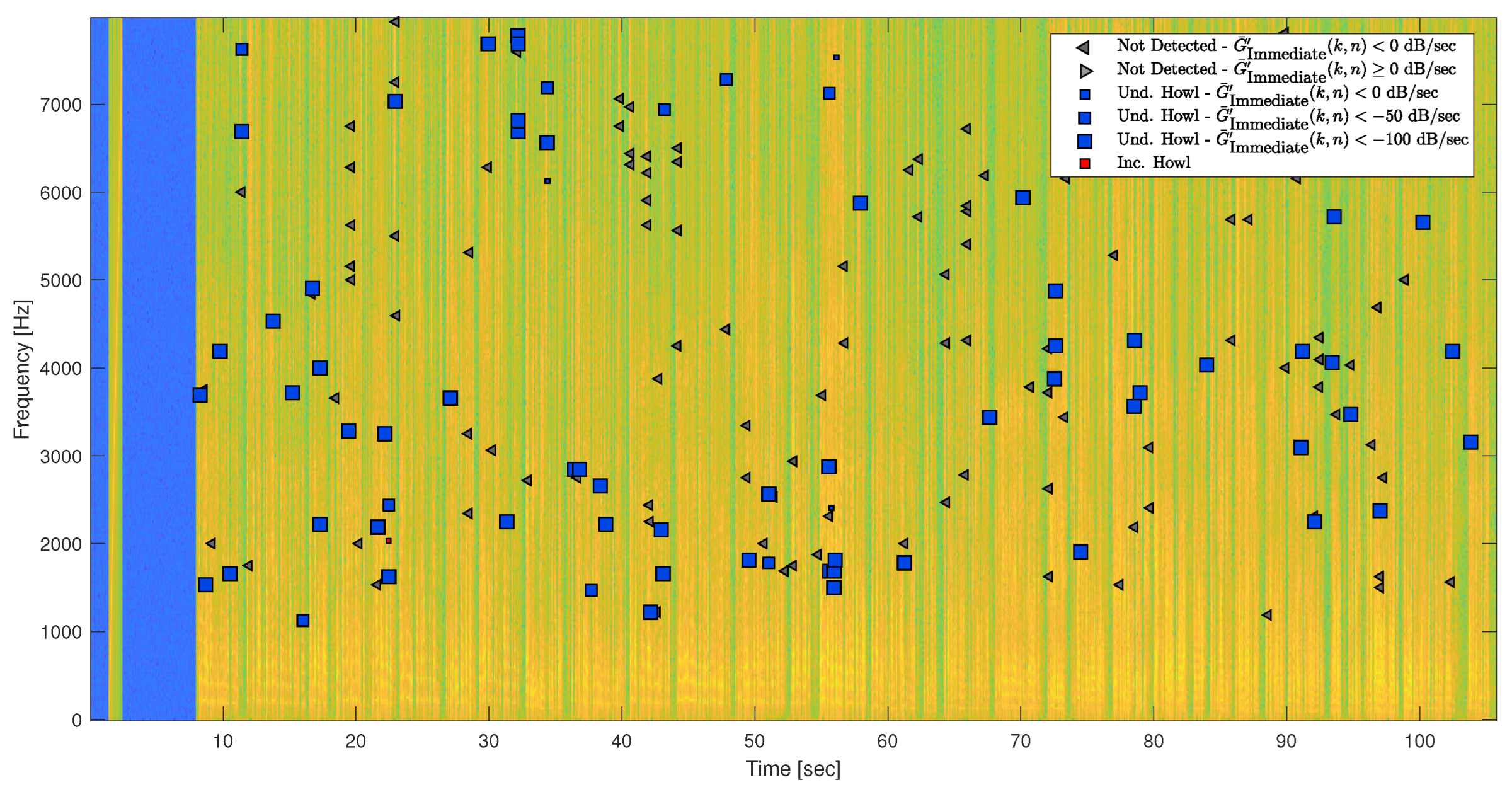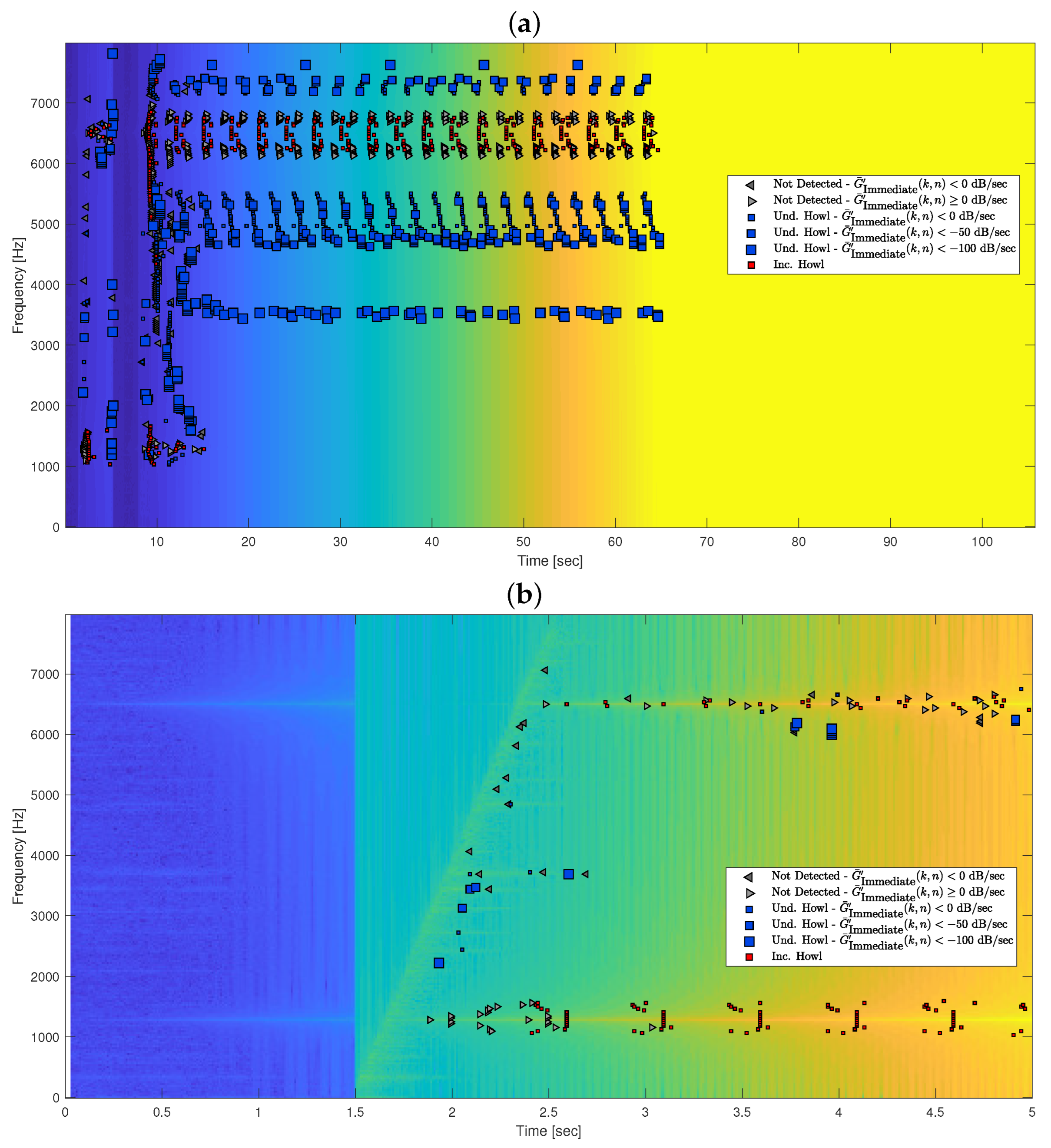The cherry-picked set of room configurations includes a car cabin, characterized as a relatively small room (short LEM paths) with a very short reverberation time (due to the sound-absorbing materials), and a study room, which is larger and has a longer reverberation time (although still short), where the MSG is obtained empirically for each room configuration [2,3,4,5], see Appendix B. Such simulated TFs provide complex feedback scenarios, consisting of Stable Poles and Close Stable Poles and, above the MSG, also Unstable Poles and More Unstable Poles. That is, while amplification gain values below the MSG may produce underdamped frequency-howls, amplification gain values above the MSG may provide a mixture of underdamped and increasing frequency-howls. Note that above the MSG, once the output signal exceeds the dynamic range of the computer due to a certain unstable pole, the magnitude values of other frequency bins are affected as well, and the howling effect of other poles cannot be analyzed. Therefore, considering that the poles of a simulated TF are unknown, only retrieved howling detections can be used for performance evaluation.

6.2.2. Accuracy Performance Evaluation

Knowing whether a detected frequency-howl is a true-positive or a false-positive, requires mapping the howling frequencies of the system, i.e., retrieving a ground truth from the output signal regarding the sensitive TF pole frequencies. For underdamped frequency-howls, the sensitive frequency bins can be triggered using a chirp signal, followed by silence to analyze the response. For increasing frequency-howls, even low-level thermal noise can trigger divergence within the system, i.e., excite the unstable poles of the closed-loop system TF. Therefore, the frequency-howl ground truth shall be obtained using a chirp signal. Similar to the energy burst in Section 6.1, the chirp signal needs to cover each frequency bin for a short, yet adequate, time span. Exploiting the fact that no false-positive frequency-howls can appear after an energy burst within a frequency bin, a sensitive howling detector shall be utilized to obtain the ground truth. Specifically, a howling detector that successfully identifies true frequency-howls, even at the cost of identifying false frequency-howls that have a similar temporal behavior along the spectrum, e.g., speech harmonics. After obtaining the frequency-howl ground truth, retrospectively detected frequency-howls can be reviewed with regard to the ground truth, and false-positive detections can be disclosed. Since the howling detector’s performance evaluation can only be conducted using retrieved instances, it is evaluated in terms of precision and recall. Identifying the relevant frequency-howl candidates via a sensitive howling detector provides data for a posterior classification, where labeling true and false frequency-howl candidates is done with respect to whether a corresponding frequency bin is flagged by the ground truth. Hence, the recall of an examined howling detector is calculated as the number of true-positive instances that were retrieved, over the number of true frequency-howl candidates. On the other hand, the precision is calculated as the number of true-positive instances that were retrieved, over the number of the entire retrieved positive instances.

For all of the above reasons, the devised input signal is responsible for composing a valid frequency-howl ground truth under the analyzed feedback scenario, and for retrieving enough howling detection instances to create a legitimate corpus, so the number of false-positive detections is negligible within ground-truth frequency bins. Therefore, the devised input signal consists of a silence preamble to fill up the history-buffer (as in Section 6.1), a chirp signal followed by silence, another silence preamble to initialize the history-buffer, and the entire long-duration speech signal used in Section 6.1. Considering a sampling frequency of 16 kHz, the chirp signal varies linearly between 200 and 7800 Hz for a duration of 1 s, and is followed by 4 s of silence in order to identify the howling frequency bins of the SR system under the given feedback scenario. Then, the test speech signal lasts for about 98 s, providing the opportunity to detect a variety of howling instances. Respectively, the simulated TF is first applied during the preamble, the 1-second chirp signal and the following 2.5 s of silence. Then, a neutral TF ($\mathrm{TF}\left(s\right)=1$) is applied during 1.5 s of silence, to suppress any evoked frequency-howl. After that, the simulated TF is applied for the rest of the input signal—the additional silence preamble and the long-duration speech signal.

6.2.3. Evaluating Multiple Detection Methods

In practice, comparing multiple howling detection methods, where each may divide the frequency and time domains differently, may result in detecting a specific frequency-howl at different times and frequencies. Therefore, a united corpus of howling detection instances is created by appending the retrospective howling detections from all detection methods. Before analyzing a given temporal detection method with respect to the united howling detection corpus, one must first match the frequencies of the howling instances to the frequency bins determined by the given method. For a given decreased-resolution method, the howling frequencies are rounded (down) to fit the frequency grid, and duplicates are dropped. For a given increased-resolution method, the howling instances are duplicated based on their resolution ratio, to fit the middle frequency bins. Appropriately, one must also match the detection times of the instances to the determined time division. Specifically, reviewing the detection times for each howling frequency, finding the relevant frame indices, and solving duplicates by choosing the instance with the frame length closest to that of the given method. Thus, the spectrogram of the devised input signal is calculated based on the parameters of the given temporal method, getting the magnitude history of the entire signal. After that, for each howling frequency bin, evaluating the magnitude history buffers ending at each of the matched detection times, via the given detection method. Regarding the duplicated howling instances, in case of an increased-resolution method, the howling detection labels are united, where at least one of the duplicated instances is hopefully detected. Finally, since simulating complex feedback scenarios, each detector’s performance is evaluated separately for underdamped and increasing frequency-howls.

7. Results

In proposing an improved howling detector that includes the Soft Howling Detection and the Howling False-Alarm Detection stages, its performance should be evaluated in comparison with that of the plain MSD-based detector in Section 4.3, as well as to that of the Soft Howling Detection stage alone. When comparing the detection response time measure, the gain-change coping mechanism, discussed in Section 5.4, is applied to the improved howling detector and evaluated as well. That is, shortening the length of the history-buffer to $N_{\mathrm{History},\mathrm{Post-Detection}}$. Hence, the examined howling detection methods are denoted as Plain MSD-based, Soft MSD-based, Soft MSD-based with FA (False-Alarm) Detection, and Soft MSD-based with FA Detection & GC (Gain-Change) Coping.

7.1. Detection Response Time

As described in Section 6.1, characterizing the response time of a howling detector involves testing two-pole TFs with poles at frequencies between 2000 and 6750 Hz, and magnitudes that correspond to change rates from −1000 to 1500 dB/s; under the five howling scenarios: Impulse Response Howl, Speech Howl, Full Stability Gain-Control Howl, Recovery Gain-Control Howl, and Increasing Gain-Control Howl. In this manner, for each combination of these three aspects, inserting a devised input signal and acquiring the first howling detection time relative to the energy burst, i.e., the response time. As mentioned in Section 6.1, for the four howling scenarios that involve inserting speech samples, the median response time is calculated. In effect, for each howling scenario, the response time of a howling detector is characterized by examining the response time distribution among all pole frequencies, across the different howling change-rate configurations.

The response time distributions over the set of howling change-rate configurations, are illustrated in Figure 6 for each howling scenario.

As expected, the Soft MSD-based detector exhibits the shortest response time, across all pole frequencies and magnitudes, in all howling scenarios except in the Recovery Gain-Control Howl scenario (Figure 6d), where the Plain MSD-based detector seems to provide a shorter response time for signal change rates above 1300 dB/s. Specifically, above 1300 dB/s, the 0.5 s before the energy burst are not enough for the neutral two-pole TF (−3000 dB/s) to eliminate the evoked howl. The fast response time of the Soft MSD-based detector lies in the fact that it has a shorter detection-buffer than the Plain MSD-based detector, and its thresholds are more permissive. In both Figure 6a,b, the Soft MSD-based with FA Detection detector provides an earlier detection time than the Plain MSD-based detector, for both negative and positive signal-magnitude change rates. For 0 dB/s (Unstable Pole), there seems to be a variance in the detection time among the pole frequencies. Figure 6c–e relate to the Gain-Control Howl scenarios. In the Full Stability Gain-Control Howl scenario, Figure 6c, it appears that the Soft MSD-based with FA Detection detector provides a faster reaction than the Plain MSD-based detector for most configured signal-magnitude change rates, except for −300, −250, and 0 dB/s. Fortunately, the gain-change coping mechanism succeeds in providing a faster response time for the first two change rates. In the Recovery Gain-Control Howl scenario, Figure 6d, it seems that the Soft MSD-based with FA Detection detector fails to provide a faster reaction than the Plain MSD-based detector for all positive-configured signal-magnitude change rates (Unstable and More Unstable Poles). However, the gain-change coping mechanism succeeds in providing a much faster howling detection for these change rates, although compromising the response time for some of the Close Stable Poles. Finally, in the Increasing Gain-Control Howl scenario, Figure 6e, the Soft MSD-based with FA Detection detector provides a shorter response time than the Plain MSD-based detector for the negative configured change rates and for the positive change rates above 140 dB/s. For the configured change rates of 0 dB/s and between 90 and 130 dB/s, the Plain MSD-based detector provides better results. As expected, the gain-change coping mechanism succeeds to improve the howling detection response times.

7.2. Detection Accuracy

First, evaluation of the detectors’ false-alarm rate over a clean signal relies on the fact that no howling artifacts should be identified. Therefore, measuring the average number of identified howling instances per second, for both howling types. For the devised input signal, with a total duration of 105.75 s, the Plain MSD-based has detected no frequency-howls from both types, as expected. While the Soft MSD-based detector has identified 224 underdamped howling artifacts and 2 increasing howling artifacts, the Soft MSD-based with FA Detection detector has identified 92 and 2 artifacts, correspondingly. That is, there is an improvement in the false-alarm rate, from 2.118 howls per second to 0.87 howls per second. The false-alarm rate improvement is illustrated in Figure 7.

It seems that most of the identified frequency-howls are underdamped, as well as the false alarms detected by the FA Detection stage.

The united corpus of howling detection instances, for obtaining the ground truth and the relevant frequency-howl candidates, is created by appending the retrospective howling detections from both the Plain MSD-based and Soft MSD-based detectors, which differ in their spectral and temporal resolutions. Accordingly, the detection accuracy results for each feedback scenario within the simulated room configurations are shown in Figure 8, where both axes are aimed to be maximized. Regarding the detectors’ performance for the feedback scenarios below the MSG (cyan-colored squares), it seems that the FA Detection stage provides better precision than the Soft Howling Detection stage by itself, while still having a good recall (above 80%) for the detection of underdamped howls. Regarding the detectors’ performance for the feedback scenarios above the MSG, specifically the detection of increasing howls (pink-colored circles), while both the Soft MSD-based and the Soft MSD-based with FA Detection detectors achieve a recall and precision of approximately 100% for the simulated car cabin, the precision is lower for all detectors within the simulated study room. However, the recall is still high and the precision is improved when using the FA Detection stage. As amplification gain values above the MSG may provide a mixture of underdamped and increasing frequency-howls, the feedback scenario within the simulated study room comprises underdamped frequency-howls as well. In that case, the Soft MSD-based with FA Detection detector achieves a lower recall and precision, although not significantly. On the other hand, the Plain MSD-based detector has identified only a few underdamped frequency-howls. Figure 9 illustrates the howling artifacts, retrospectively detected via the Soft MSD-based with FA Detection detector, in case of the simulated study room above the MSG. Many underdamped frequency-howls that were detected during the speech signal were not detected as ground truth by the chirp signal.

8. Discussion

The proposed performance evaluation framework compares the group of howling detection techniques in terms of both the response time and detection accuracy. The generic TF approach is applied in order to analyze the response time of a howling detector under each of the devised set of howling scenarios, illustrating the detection response time distributions over the set of howling change-rate configurations. In the simple howling scenarios, the Soft MSD-based with FA Detection detector provides a faster howling detection response time than the Plain MSD-based detector, especially in Close Stable Pole feedback scenarios. The advantage of a shortened history-buffer in these scenarios, as used in the Soft MSD-based with FA Detection & GC Coping detector, is not absolute for all feedback scenarios. Nevertheless, the improvement by the gain-change coping mechanism is significant in Gain-Control Howl scenarios for the Close Stable Pole feedback scenarios, although not much better than the Plain MSD-based detector in the More Unstable Pole feedback scenarios. Since aiming to detect howling before the SR system becomes unstable, the improvement in detection response time is more significant for Close Stable Pole feedback scenarios.

The Detection Accuracy is measured in terms of the false-alarm rate over a clean signal, and the detectors’ recall and precision in complex feedback scenarios, generated by simulating a simple SR system TF in a cherry-picked set of room configurations. Regarding the clean signal, almost 60% of the false-positive underdamped frequency-howls detected in the Soft Howling Detection stage are refuted by the Howling FA Detection stage. However, the two false-positive increasing frequency-howls were not refuted. Regarding the detection accuracy in complex feedback scenarios below the MSG, the FA Detection stage improves the precision of the Soft Howling Detection stage, while keeping a good recall for the detection of underdamped howls. In feedback scenarios above the MSG, the FA Detection stage resulted in better recall and precision measurements for increasing howls, although the precision for underdamped howls was low for all detectors within the simulated study room. As mentioned above, a few aspects need to be considered in this case. First, the diverging output signal has affected the magnitude values among the entire frequency bins, and has possibly added artifacts to the signal that were identified as howling. In addition, it seems that the howling detectors were not sensitive enough to obtain all of the frequency-howl ground truth in this scenario. Thus, the low precision can be attributed to identifying many underdamped howls along the output signal, and not identifying all of the howling frequencies in the system at the beginning. Still, the detection accuracy of increasing howls within the More Unstable Pole feedback scenario is good.

As the algorithm thresholds were calibrated within the simulated car cabin, the better results may indicate overfitting. However, the results are satisfying for the study room as well.

9. Conclusions

We have considered a howling detection algorithm within in-room speech reinforcement system applications, for utilization in howling control mechanisms. The loudspeaker-enclosure-microphone paths and the room’s reverberation characteristics directly affect the acoustic feedback in the room, and the resonance frequencies of the system’s closed-loop TF. Therefore, the amount of gain that can be applied to the acquired speech in the closed-loop system is constrained by electro-acoustic coupling in the system, manifested in howling noises appearing as a result of acoustic feedback. In fact, these howling noises can be divided into underdamped and increasing frequency-howls, based on what happens to the frequency component of the output signal after exciting a pole of the system’s closed-loop TF. A temporal howling detection algorithm based on the MSD measure is proposed for SR systems. The proposed algorithm aims to early detect frequency-howls in the closed-loop system, before the human ear notices. Thus, laying the foundation for howling control mechanisms, and maintaining high-quality speech communication. In reality, when the applied gain is increased gradually, a howling detection algorithm mainly aims to detect underdamped frequency-howls when the system is stable, rather than increasing howls when the system is unstable. The howling detection algorithm includes two cascaded stages: Soft Howling Detection and Howling False-Alarm Detection. The Soft Howling Detection stage is designed to identify potential candidate frequency-howls, and is calibrated for a low miss-detect probability. Accordingly, the proposed Howling False-Alarm Detection stage aims to authenticate each suspected frequency-howl with regard to the signal behavior prior to detection. As the majority of howling false alarms can be attributed to frequency components of speech harmonics, candidate frequency-howl false alarms can be refuted based on their prior magnitude behavior under the system’s steady state. Furthermore, a gain-change coping mechanism is applied to appropriately manage the howling detection process when the applied gain is reduced or increased as part of a howling control mechanism. In order to judge whether a candidate frequency-howl is about to be heard by the human ear, i.e., relevant for howling detection, a hearing threshold-contour is defined across the frequency bins based on standard ISO 226:2003 [23].

A comprehensive performance evaluation process was designed to characterize and compare a group of howling detection algorithms, under a devised set of howling detection scenarios. Namely, examining the howling detection algorithms in terms of the detection response time and the detection accuracy. First, characterizing the howling detection response time as a function of howling change rate, under different howling detection scenarios, shows that the proposed algorithm provides a faster howling detection response time than the plain MSD-based detector; and that the improvement of the gain-change coping mechanism is significant in the gain-control scenarios for underdamped feedback scenarios. Second, evaluating the detection accuracy on a clean test signal and under complex stable- and unstable-feedback scenarios, within simulated room configurations of a car cabin and a study room, shows that the proposed temporal howling detection algorithm provides better accuracy than the plain MSD-based detector as well as the Soft Detection stage alone. Hence, the proposed temporal howling detection algorithm is fast and reliable and, all in all, outperforms the plain howling detector, which does not benefit from utilizing the past of the detected frequency-howls due to its prominent trade-offs.

Future work may concern optimizing the thresholds of the proposed howling detection algorithm for each type of room configuration, e.g., room dimensions and reverberation time. Moreover, incorporating more advanced algorithms for howling detection that make use of the proposed temporal approach and features.