Compensation of Modeling Errors for the Aeroacoustic Inverse Problem with Tools from Deep Learning

Abstract

In the field of aeroacoustic source imaging, one seeks to reconstruct acoustic source powers from microphone array measurements. For most setups, one cannot expect a perfect reconstruction. The main effects that contribute to this reconstruction error are data noise and modeling errors. While the data noise is accounted for in most advanced reconstruction methods, e.g., by a proper regularization strategy, the modeling error is usually neglected. This article proposes an approach that extends regularized inverse methods with a mechanism that takes the modeling error into account. The presented algorithmic framework utilizes the representation of the Fast Iterative Shrinkage Thresholding Algorithm (FISTA) algorithm by a neural network and uses standard gradient schemes from the field of deep learning. It is directly applicable to a single measurement, i.e., a prior training phase on previously generated data is not required. The capabilities of the method are illustrated by several numerical examples.

1. Introduction

Reconstruction of acoustic sources from aeroacoustic measurements has been an active field of research for many decades [1,2,3,4,5]. As aeroacoustic measurements are usually conducted in environments that are subject to random processes (such as wind tunnels), reconstruction procedures are usually based on cross spectral data, i.e., correlations in the frequency domain. There exist various source power reconstruction methods for correlation data such as Beamforming (see, e.g., [6]), CLEAN-SC [7], DAMAS [8] or Covariance Matrix Fitting also known as CMF (see, e.g., [9,10]). In this article, we will present an approach based on a regularized version of CMF.

Usually, source power estimations can only provide an approximation of the ground truth source powers, and there are two main causes for this reconstruction error. Firstly, data noise, which can be treated by suitable regularization. Secondly, modeling errors, i.e., usage of a physical sound propagation model that does not exactly match to conditions of the measurement environment. In this article, we present an approach that extends regularized CMF with additional degrees of freedom (DOFs) in order to take modeling errors into account. Here, we will only consider additional DOFs for the phase of the sound propagation matrix, as this is much more affected by modeling errors than the amplitudes. The proposed method is based on the Fast Iterative Shrinkage Thresholding Algorithm (FISTA) optimization algorithm, originally proposed by Beck & Teboulle for ${\ell }^1$-regularized least squares [11], which is an accelerated version of the iterative shrinkage-thresholding (ISTA) algorithm (see, e.g., [12,13]). Several variants of this algorithm have also been applied in the field of aeroacoustics [14,15,16,17]. Moreover, the principle of unrolling is used here. Unrolling means that a fixed number of (F)ISTA iterations is represented by a neural network, where the number of layers matches the number of (F)ISTA iterations (see, e.g., [18]).

As we employ tools from machine learning, in particular deep learning, we would like to relate our approach to other data-driven methods in inverse problems, respectively, acoustic source imaging. On the one hand, there exist purely data-driven approaches that fully learn the source power reconstruction [19,20,21,22]. Our approach is a hybrid one, i.e., it combines model-based methods with principles from machine learning. Other hybrid approaches in inverse problems are, for example, learned regularizers [23,24] or learned operator correction [25]. The concept of unrolling, which can also be seen as an hybrid approach, has been employed for Learned ISTA (LISTA) [26,27] and Trainable ISTA (TISTA) [28,29], which both optimize or learn some parameters of the ISTA algorithm. The latter one has recently been applied to acoustic source imaging [30]. The main principle for the compensation of the modeling error effects used in this work is motivated by ideas from Regularized Total Least Squares [31,32] and the Deep Inverse Prior [33]. The regularized cost function that measures the data misfit between modeled and measured data is optimized not only with respect to the source powers but additionally with respect to sound propagation parameters. In contrast to most machine learning frameworks, this approach does not include a prior training period on previously simulated or measured training data. Hence, it can be applied to a single measurement. We would like to emphasize that in this article, we focus on the presentation of the main ideas and a proof of concept to estimate the capabilities of the method. Hence, this is only the first step towards an applicability for real measurement scenarios.

2. Problem Modeling

Let c denote the speed of sound, $\mathbf{u}\in {\mathbb{R}}^3$ a constant convection field, and $\mathbf{m}=\frac{\mathbf{u}}{c}$ the Mach vector. Moreover, we consider subsonic convection, i.e., it is assumed that ${∥\mathbf{m}∥}_2<1$. The standard sound propagation model that is employed in experimental aeroacoustics is the convected Helmholtz equation which describes time harmonic sound propagation within the convection field $\mathbf{u}$

$${(k-i\mathbf{m}·\nabla )}^{2}p+\Delta p=-s.$$

(1)

In Equation (1), $k=\frac{\omega }{c}$ denotes the wavenumber, where $\omega =2\pi f$ the angular frequency and f the frequency. Further, p denotes the complex pressure field and s a generic source. Note that the time factor convention $e^{+i\omega t}$ is used. The free field Green’s function for the convected Helmholtz equation is given by

$$\begin{array}{c}\hfill g(\mathbf{x},\mathbf{y})=\frac{\exp \left(\frac{-ik}{1-{∥\mathbf{m}∥}_2^2}\left(-(\mathbf{x}-\mathbf{y})·\mathbf{m}+{∥\mathbf{x}-\mathbf{y}∥}_{\mathbf{m}}\right)\right)}{4\pi {∥\mathbf{x}-\mathbf{y}∥}_{\mathbf{m}}}.\end{array}$$

(2)

where the Mach norm is defined by

$$\begin{array}{c}\hfill {∥\mathbf{z}∥}_{\mathbf{m}}=\sqrt{{\left(\mathbf{z}·\mathbf{m}\right)}^2+{\beta }^2{∥\mathbf{z}∥}_2^2},\end{array}$$

with ${\beta }^2=1-{∥\mathbf{m}∥}_2^2$. Although the formulation (2) ignores any geometric features of the measurement setup (e.g., presence of walls), the free field Green’s function is widely used for source power reconstruction in experimental aeroacoustics as it provides robust results.

The discrete forward model is set up as follows. The map domain, i.e., the regions where sources are assumed is discretized by N focus positions ${\mathbf{y}}_1,\dots ,{\mathbf{y}}_N$ and the positions of the array microphones are denoted by ${\mathbf{x}}_1,\dots ,{\mathbf{x}}_M$. The pressure signal at the array and the source signal at the focus positions are given by

$$\begin{array}{c}\hfill \mathbf{p}\left(\omega \right)=\left(\begin{array}{c}p({\mathbf{x}}_1,\omega )\\ ⋮\\ p({\mathbf{x}}_M,\omega )\end{array}\right)\mathrm{and}\mathbf{s}\left(\omega \right)=\left(\begin{array}{c}s({\mathbf{y}}_1,\omega )\\ ⋮\\ s({\mathbf{y}}_N,\omega )\end{array}\right).\end{array}$$

As the measurement environment is subject to random processes, both the pressure signal $\mathbf{p}\left(\omega \right)\in {\mathbb{C}}^{\mathbb{M}}$ and the source signal $\mathbf{s}\left(\omega \right)\in {\mathbb{C}}^{\mathbb{N}}$ are considered as random variables with zero mean. The propagation matrix $\mathbf{G}\in {\mathbb{C}}^{M\times N}$ defined by

$${\mathbf{G}}_{mn}=g({\mathbf{x}}_m,{\mathbf{y}}_n),$$

(3)

determines the linear relation between source and array signal

$$\mathbf{p}=\mathbf{G}\mathbf{s}.$$

Taking the correlation matrix of $\mathbf{p}$, we obtain

$$\mathbf{C}:=\mathbb{E}\left\{\mathbf{p}{\mathbf{p}}^H\right\}=\mathbf{G}\mathbb{E}\left\{\mathbf{s}{\mathbf{s}}^H\right\}{\mathbf{G}}^H,$$

where H denotes the Hermitian transpose. The matrix $\mathbf{C}$ is usually denoted as cross spectral matrix (CSM). A standard assumption in experimental acoustics, which will also be employed here, is the assumption of spatially uncorrelated sources. This means that the correlation matrix of the source signal is given by a diagonal matrix, i.e.,

$$\mathbb{E}\left\{\mathbf{s}{\mathbf{s}}^H\right\}={\mathbf{M}}_{\mathbf{q}}=\mathrm{diag}\left({\mathbf{q}}_1,\dots ,{\mathbf{q}}_N\right)\mathrm{with}\mathbf{q}={\left(\mathbb{E}\left\{|{\mathbf{s}}_1{|}^2\right\},\dots ,\mathbb{E}\left\{|{\mathbf{s}}_N{|}^2\right\}\right)}^{\top }.$$

The vector $\mathbf{q}$ will be denoted as source power vector in the following. Finally, the discrete inverse problem can be stated as follows: given a CSM $\mathbf{C}\in {\mathbb{C}}^{M\times M}$, find a source power vector $\mathbf{q}\in {\mathbb{R}}^N$ such that

$$\mathbf{G}{\mathbf{M}}_{\mathbf{q}}{\mathbf{G}}^H=\mathbf{C}.$$

For the further analysis, we introduce the discrete forward operator

$$\mathcal{C}\left(\mathbf{q}\right)=\mathbf{G}{\mathbf{M}}_{\mathbf{q}}{\mathbf{G}}^H$$

(4)

and its adjoint operator

$${\mathcal{C}}^{\ast }\left(\mathbf{K}\right)=\mathrm{diag}\left({\mathbf{G}}^H\mathbf{K}\mathbf{G}\right),\mathrm{for}\mathbf{K}\in {\mathbb{C}}^{M\times M}.$$

(5)

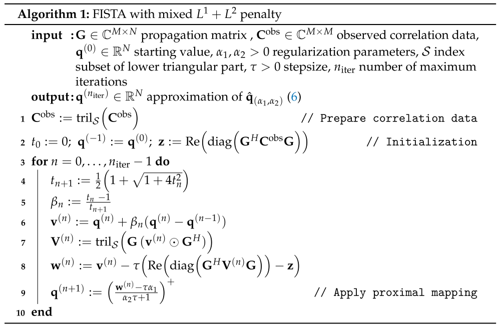
3. Source Power Reconstruction with FISTA

For real experimental data, only a noisy approximation ${\mathbf{C}}^{\mathrm{obs}}$ of the true CSM $\mathbf{C}$ is available. Therefore, an appropriate source power reconstruction technique is the following regularized version of Cross Spectral Matrix Fitting (CMF) [9,10]

$${\widehat{\mathbf{q}}}_{({\alpha }_1,{\alpha }_2)}=\underset{\mathbf{q}\ge 0}{argmin}\frac{1}{2}{∥\mathbf{G}{\mathbf{M}}_{\mathbf{q}}{\mathbf{G}}^H-{\mathbf{C}}^{\mathrm{obs}}∥}_F^2+\mathcal{R}\left(\mathbf{q}\right),$$

(6)

where the penalty functional $\mathcal{R}$ is given by

$$\mathcal{R}\left(\mathbf{q}\right)={\alpha }_1{∥\mathbf{q}∥}_1+{\alpha }_2\frac{1}{2}{∥\mathbf{q}∥}_2^2$$

and ${\alpha }_1,{\alpha }_2\ge 0$ denote the regularization parameters. The $L1$ penalty promotes a sparse source power vector, which is a realistic assumption for many aeroacoustic measurements. The $L2$ penalty ensures that the minimization problem has a unique solution. The objective function in Equation (6) can be efficiently minimized using the framework of the generalized Fast Iterative Shrinkage Thresholding Algorithm (FISTA) (p. 291, [34]). The principle of the FISTA algorithm is to repeat an alternating application of the following two operations:

• A gradient step with respect to the first summand of the objective function;
• Application of the proximal mapping (see Definition 6.1, p. 129, [34]) of the regularization part.

An implementation of this generic method for the specific problem (6) is given in Algorithm 1.

We conclude this section with some remarks on the implementation.

• The most expensive step in Algorithm 1 is the evaluation of ${\mathcal{C}}^{\ast }\mathcal{C}$, which corresponds to line 7 and 8. By exploiting the multiplicative structure (see Equations (4) and (5)), this can be implemented efficiently (see [35]).
• To ensure convergence, the step size $\tau$ must satisfy

  $$\tau <{\left(\underset{\mathbf{q}\in {\mathbb{R}}^N,x\ne 0}{sup}\frac{{∥{\mathcal{C}}^{\ast }\mathcal{C}\left(\mathbf{q}\right)∥}_2}{{∥x∥}_2}\right)}^{-1},$$

  where the upper bound may be estimated, e.g., by the power method (see p. 239, [36]).
• As the observed CSM ${\mathbf{C}}^{\mathrm{obs}}$ is Hermitian, the upper diagonal part can be neglected. Therefore, $\mathcal{S}$ denotes the index set of the lower triangular part of the CSM. The operation ${\mathrm{tril}}_{\mathcal{S}}\left((\right)·)$ sets all entries to zero that do not belong to $\mathcal{S}$. Moreover, the principle of diagonal removal can be easily incorporated by defining $\mathcal{S}$ as the lower triangular indices without the diagonal.
• The operation ${\mathbf{v}}^{\left(n\right)}\odot {\mathbf{G}}^H$ multiplies each column of ${\mathbf{G}}^H$ component-wise by the vector ${\mathbf{v}}^{\left(n\right)}$.
• The operation ${(·)}^{+}$ takes the positive part component-wise, i.e., ${\left(x\right)}^{+}=max(x,0)$.

4. Optimization of Phase Modeling Parameters

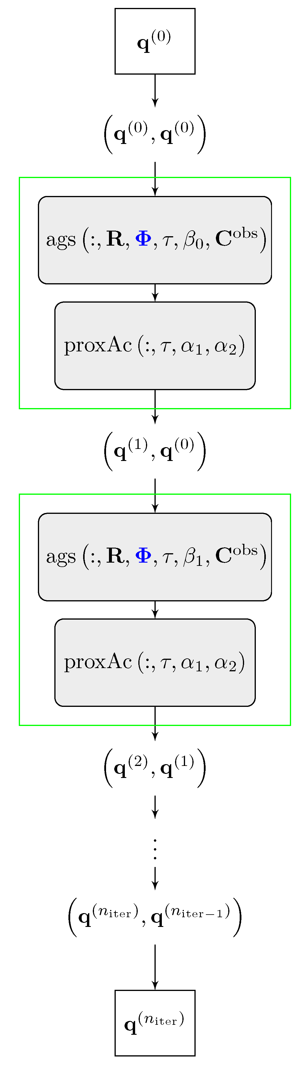
For most measurement scenarios, the free-field sound propagation matrix $\mathbf{G}$ (Equations (2) and (3)) is only an approximation of the true sound propagation. In this section, we will derive a framework that adds more degrees of freedom to the reconstruction process in order to compensate for this modeling error. Note that the propagation matrix $\mathbf{G}$ can be expressed as

$$\mathbf{G}=\mathbf{R}\odot exp\left(i\Phi \right),$$

where $\mathbf{R},\Phi \in {\mathbb{R}}^{M\times N}$ are the amplitude and phase matrices, respectively, ⊙ denotes the component-wise or Hadamard product and the exponential also operates component-wise. For the entire article, we assume that the amplitude matrix $\mathbf{R}$ is sufficiently well known but the phase matrix $\Phi$ is perturbed by a modeling error. In most measurement scenarios, the modeling of $\mathbf{R}$ is usually much more accurate than the modeling of the phase.

4.1. Unrolled FISTA

Let $\mathbf{R}$ be given and fixed, then for each phase matrix $\Phi$, we can define the corresponding Tikhonov minimizer

$$\widehat{\mathbf{q}}(\Phi )=\underset{\mathbf{q}\ge 0}{argmin}\frac{1}{2}{∥\left[\mathbf{R}\odot exp\left(i\Phi \right)\right]{\mathbf{M}}_{\mathbf{q}}{\left[\mathbf{R}\odot exp\left(i\Phi \right)\right]}^H-{\mathbf{C}}^{\mathrm{obs}}∥}_F^2+\mathcal{R}\left(\mathbf{q}\right).$$

(7)

As outlined in the last section, this minimizer can be efficiently approximated by $n_{\mathrm{iter}}$ steps of the FISTA algorithm (see Algorithm 1). Moreover, the FISTA algorithm with a fixed number of iterations can be regarded as the application of a neural network $\mathcal{F}$ with $n_{\mathrm{iter}}$ layers. The general principle of representing iterative optimization algorithms as neural networks is usually referred to as algorithm unrolling. For an extensive review on the principle of algorithm unrolling, we refer to the review article [18]. The specific case that is employed here (unrolling the FISTA algorithm), will be described in detail below.

For the computation of one FISTA iteration, one needs the pair of the last two iterates, denoted by $(\mathbf{q},{\mathbf{q}}^{\prime })$ in the following. Lines 6–8 in Algorithm 1 perform the accelerated gradient step. The computation of each line can be represented by a corresponding function

$$\begin{array}{cc}\hfill \mathrm{ag}1\left((\mathbf{q},{\mathbf{q}}^{\prime }\right),\beta )& =\mathbf{q}+\beta (\mathbf{q}-{\mathbf{q}}^{\prime }),\hfill \\ \hfill \mathrm{ag}2(\mathbf{v},\mathbf{R},\Phi )& ={\mathrm{tril}}_{\mathcal{S}}\left(\left[\mathbf{R}\odot exp\left(i\Phi \right)\right](\mathbf{v}\odot {\left[\mathbf{R}\odot exp\left(i\Phi \right)\right]}^H)\right),\hfill \\ \hfill \mathrm{ag}3\left(\mathbf{v},\mathbf{V},\mathbf{R},\Phi ,\tau ,{\mathbf{C}}^{\mathrm{obs}}\right)& =\mathbf{v}-\tau \mathrm{Re}\left(\mathrm{diag}\left({\left[\mathbf{R}\odot exp\left(i\Phi \right)\right]}^H\left[\mathbf{V}-{\mathbf{C}}^{\mathrm{obs}}\right]\left[\mathbf{R}\odot exp\left(i\Phi \right)\right]\right)\right).\hfill \end{array}$$

The entire accelerated gradient step can be represented by a concatenation of the functions defined above

$$\begin{array}{c}\hfill \mathrm{ags}\left((\mathbf{q},{\mathbf{q}}^{\prime }),\mathbf{R},\Phi ,\tau ,\beta ,{\mathbf{C}}^{\mathrm{obs}}\right)=\left(\mathrm{ag}3\left(\mathrm{ag}1(\mathbf{q},{\mathbf{q}}^{\prime },\beta ),\mathrm{ag}2(\mathbf{v},\mathbf{R},\Phi ),\mathbf{R},\Phi ,\tau ,{\mathbf{C}}^{\mathrm{obs}}\right),\mathbf{q}\right).\end{array}$$

(8)

Note that the function $\mathrm{ags}$ (8) is linear with respect to its first argument. In the context of neural networks, line 9 of Algorithm 1 can be interpreted as the application of a non-linear activation function. For a pair of vectors $(\mathbf{w},\mathbf{q})$, we therefore define the activation function of the neural network as

$$\begin{array}{c}\hfill \mathrm{proxAc}\left((\mathbf{w},\mathbf{q}),\tau ,{\alpha }_1,{\alpha }_2\right)=\left({\left(\frac{\mathbf{w}-\tau {\alpha }_1}{{\alpha }_2\tau +1}\right)}^{+},\mathbf{q}\right).\end{array}$$

(9)

Note that the activation function $\mathrm{proxAc}$ (9) applies the nonlinear proximal mapping on the first component $\mathbf{w}$ and simply keeps the second component q, as the previous two iterates are needed for the next FISTA iteration.

With the propagation function $\mathrm{ags}$ (8) and the activation function $\mathrm{proxAc}$ (9), we can interpret the FISTA algorithm as a feed-forward neural network with the following characteristics:

• The set of trainable parameters of $\mathcal{F}$ are the entries of the phase matrix $\Phi$. Those are shared for each layer. Note that the set of trainable and non-trainable parameters can be varied but we will restrict our investigations to the case where $\Phi$ is trainable.
• The starting value ${\mathbf{q}}^{\left(0\right)}$ is the data input of the neural network and is transformed to the pair $\left({\mathbf{q}}^{\left(0\right)},{\mathbf{q}}^{\left(0\right)}\right)$ before the first layer.
• The network consists of $n_{\mathrm{iter}}$ layers, where each layer represents one FISTA iteration. In each layer, the following two operations are applied to the pair $\left(\mathbf{q},{\mathbf{q}}^{\prime }\right)$:

  1.

  The current pair is propagated forward by linear operations, encoded in $\mathrm{ags}$ (8), which essentially depend on the trainable parameters $\Phi$ and the non-trainable parameters $\mathbf{R},{\mathbf{C}}^{\mathrm{obs}},\tau ,{\beta }_n,{\alpha }_1,{\alpha }_2$.

  2.

  After the propagation step, the activation function $\mathrm{proxAc}$ (9) is applied.

• After the last layer, the output pair $\left({\mathbf{q}}^{\left(n_{\mathrm{iter}}\right)},{\mathbf{q}}^{\left(n_{\mathrm{iter}-1}\right)}\right)$ is transformed to the final output ${\mathbf{q}}^{\left(n_{\mathrm{iter}}\right)}$.

A sketch of the framework of the neural network $\mathcal{F}$ is presented in Figure 1.

Denote by ${\mathcal{F}}_{\Phi }\left({\mathbf{q}}^{\left(0\right)}\right)$ the output of the neural network for starting value ${\mathbf{q}}^{\left(0\right)}$ and phase parameters $\Phi$. Using this notation and the definition of the Tikhonov minimizer $\widehat{\mathbf{q}}(\Phi )$ (7), we get the approximation

$$\widehat{\mathbf{q}}(\Phi )\approx {\mathcal{F}}_{\Phi }\left({\mathbf{q}}^{\left(0\right)}\right).$$

(10)

4.2. Constrained Residual Minimization

In a scenario where the phase of the propagation is subject to a modeling error, this will affect the accuracy of the Tikhonov minimizer $\widehat{\mathbf{q}}(\Phi )$. To account for this modeling error in the minimization process, we consider the following constrained problem

$$\begin{array}{cc}\hfill & \underset{\Phi }{min}\frac{1}{2}{∥\left[\mathbf{R}\odot exp\left(i\Phi \right)\right]{\mathbf{M}}_{\widehat{\mathbf{q}}(\Phi )}{\left[\mathbf{R}\odot exp\left(i\Phi \right)\right]}^H-{\mathbf{C}}^{\mathrm{obs}}∥}_F^2\hfill \\ \hfill \mathrm{subject}\mathrm{to}\widehat{\mathbf{q}}(\Phi )=& \underset{\mathbf{q}\ge 0}{argmin}\frac{1}{2}{∥\left[\mathbf{R}\odot exp\left(i\Phi \right)\right]{\mathbf{M}}_{\mathbf{q}}{\left[\mathbf{R}\odot exp\left(i\Phi \right)\right]}^H-{\mathbf{C}}^{\mathrm{obs}}∥}_F^2+\mathcal{R}\left(\mathbf{q}\right).\hfill \end{array}$$

Using the approximation (10) and replacing the constraint, we get the following unconstrained problem

$$\underset{\Phi }{min}{∥\left[\mathbf{R}\odot exp\left(i\Phi \right)\right]{\mathbf{M}}_{{\mathcal{F}}_{\Phi }\left({\mathbf{q}}^{\left(0\right)}\right)}{\left[\mathbf{R}\odot exp\left(i\Phi \right)\right]}^H-{\mathbf{C}}^{\mathrm{obs}}∥}_F^2=:\underset{\Phi }{min}\mathcal{J}(\Phi ).$$

(11)

Note that we also omitted the factor $\frac{1}{2}$ in front of the residual as it does not affect minimizers. The problem (11) is a minimization problem with respect to the trainable neural network parameters $\Phi$. Hence, the loss function in (11) can be minimized by standard tools (i.e., gradient descent schemes) for the training of neural networks. A generic gradient descent scheme $\mathcal{G}$ receives the current network parameters, the gradient of the cost function with respect to the network parameters, the learning rate, and potentially other parameters as in input and returns the updated network parameters. Typical examples for such schemes $\mathcal{G}$ are standard gradient descent, gradient descent with momentum or ADAM [37]. The whole procedure to minimize $\mathcal{J}$ with a generic gradient descent optimizer $\mathcal{G}$ is summarized in Algorithm 2.

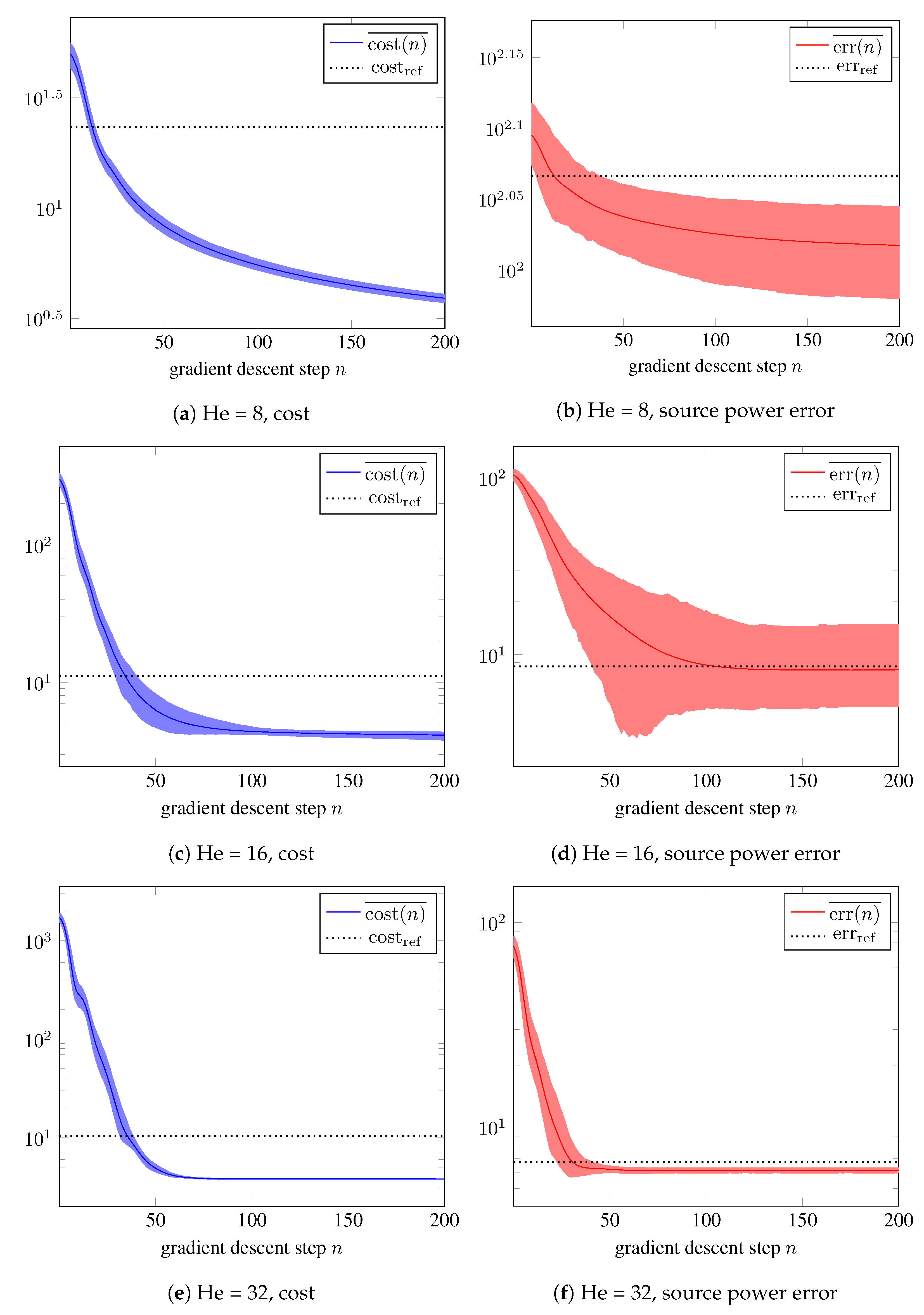
5. Numerical Examples

To examine the performance of the designed problem (11), we consider a simple numerical example with four monopole sources. This setup has also been used in previous publications for synthetic benchmark computations [38]. The microphone array has an aperture of $d=1.5$ m and consists of 64 microphones positioned in the x-y plane, where the center microphone is located at ${(0,0,0)}^{\top }$. The focus plane is positioned at $z=0.75\mathrm{m}$ with $x,y\in [-0.2\mathrm{m},0.2\mathrm{m}]$. All computations are done using an equidistant focus grid with resolution ${\Delta }_{xy}=0.02\mathrm{m}$ which results in $N=441$ focus points in total, denoted by ${\mathbf{y}}_n$.

Data generation: We consider a convective field with Mach vector $\mathbf{m}={(0.2,0,0)}^{\top }$, speed of sound $c=343\frac{\mathrm{m}}{\mathrm{s}}$. The data are generated for three Helmholtz numbers $\mathrm{He}=\frac{fd}{c}$ with values $\mathrm{He}\in \{8,16,32\}$. The exact correlation matrix, propagation matrix and source power vector are denoted by ${\mathbf{C}}^{\mathrm{exact}}\in {\mathbb{C}}^{M\times M}$, ${\mathbf{G}}^{\mathrm{exact}}\in {\mathbb{C}}^{M\times N}$ and ${\mathbf{q}}^{†}\in {\mathbb{R}}^N$. In order to generate also noisy data ${\mathbf{C}}^{\mathrm{obs}}\in {\mathbb{C}}^{M\times M}$, we draw $n_{\mathrm{samp}}=1000$ pressure samples according to

$${\mathbf{p}}^{\left(j\right)}={\mathbf{G}}^{\mathrm{exact}}\left({\eta }^{\left(j\right)}\odot \sqrt{{\mathbf{q}}^{†}}\right)+\delta {ϵ}^{\left(j\right)}\mathrm{for}j=1,\dots ,n_{\mathrm{samp}},\delta \ge 0.$$

(12)

In (12), ⊙ denotes pointwise multiplication and the vectors ${\eta }^{\left(j\right)}\in {\mathbb{C}}^M,{ϵ}^{\left(j\right)}\in {\mathbb{C}}^N$ are sampled independently from vector-valued, standard complex normal random variables $\eta$ and $ϵ$

$$\eta \sim {\left[{\mathcal{N}}_{\mathbb{C}}(0,1)\right]}^N,ϵ\sim {\left[{\mathcal{N}}_{\mathbb{C}}(0,1)\right]}^M,\eta \perp ϵ.$$

The level of the additive noise $\delta$ is chosen such that

$$\delta =\sqrt{\frac{M·0.05}{{\sum }_{m=1}^M\left|{\mathbf{C}}_{mm}^{\mathrm{exact}}\right|}}.$$

Thus, for $n_{\mathrm{samp}}\to \infty$, the average relative perturbation of the diagonal of the correlation matrix is approximately $5\%$. Noisy data are then obtained by

$${\mathbf{C}}^{\mathrm{obs}}=\frac{1}{n_{\mathrm{samp}}}\sum _{j=1}^{n_{\mathrm{samp}}}{\mathbf{p}}^{\left(j\right)}{{\mathbf{p}}^{\left(j\right)}}^H.$$

The neural network ${\mathcal{F}}_{\Phi }$ is set up using the fixed source input ${\mathbf{q}}^{\left(0\right)}={(0,\dots ,0)}^{\top }$, $n_{\mathrm{iter}}=100$ layers (i.e., FISTA iterations) and regularization parameters ${\alpha }_1={10}^{-5}$, ${\alpha }_2={10}^{-7}$ for all examples. Figure 2 shows the exact source powers and the reconstructed source powers for $\mathrm{He}=16$ using 100 FISTA iterations and the exact propagation matrix ${\mathbf{G}}^{\mathrm{exact}}$. Reconstruction with the correct propagation model leads to an reconstruction error of 7.49.

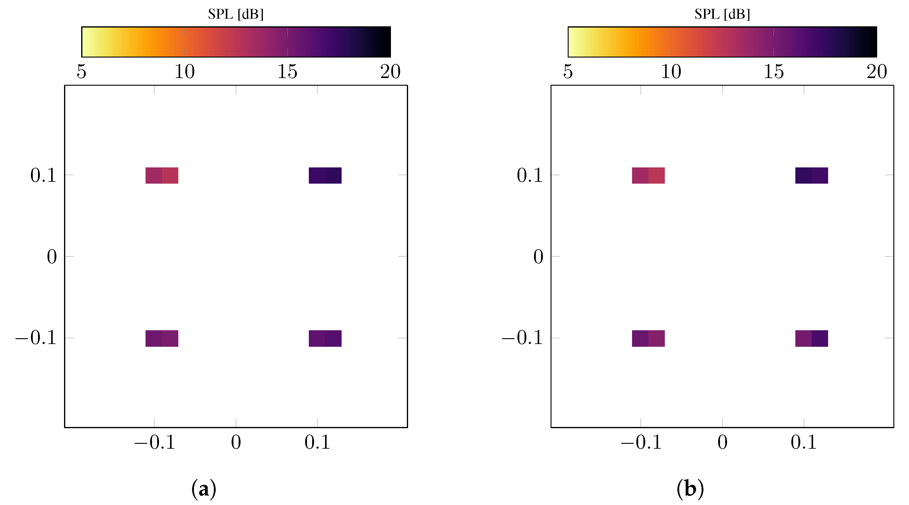
5.1. Systematic Modeling Error

As a first example, we consider a systematic phase modeling error by slightly perturbing the Mach vector by $5\%$ from $\mathbf{m}={(0.2,0,0)}^{\top }$ to $\mathbf{m}={(0.19,0,0)}^{\top }$. The resulting erroneous phase matrix is denoted by ${\Phi }^{\mathrm{syst}}$. The residual optimization (11) is done using Python and TensorFlow [39], where the used hyperparameter values are summarized in

Table 1. Hyperparameter values used for the gradient descent scheme.

Optimization algorithm	Gradient descent with Nesterov momentum (p. 353, [40])
Learning rate	lr$={10}^{-3}$
Momentum parameter	momentum$=0.9$
Gradient descent steps	$n_{\mathrm{grad}}=200$

.

Figure 3a shows the result for the FISTA reconstruction, the systematically perturbed propagation matrix $\mathbf{R}\odot exp{\Phi }^{\mathrm{syst}}$, and Figure 3b the result of the residual minimization (see (11)) with initial network parameters ${\Phi }^{\mathrm{syst}}$. We observe that the perturbed flow magnitude leads to an error in the source location. As the source grid is relatively coarse, the main peak of each source is distributed over two source grid points. This effect of the systematic model error cannot be compensated by the neural network method, i.e., both methods produce a reconstruction error of the same order of magnitude.

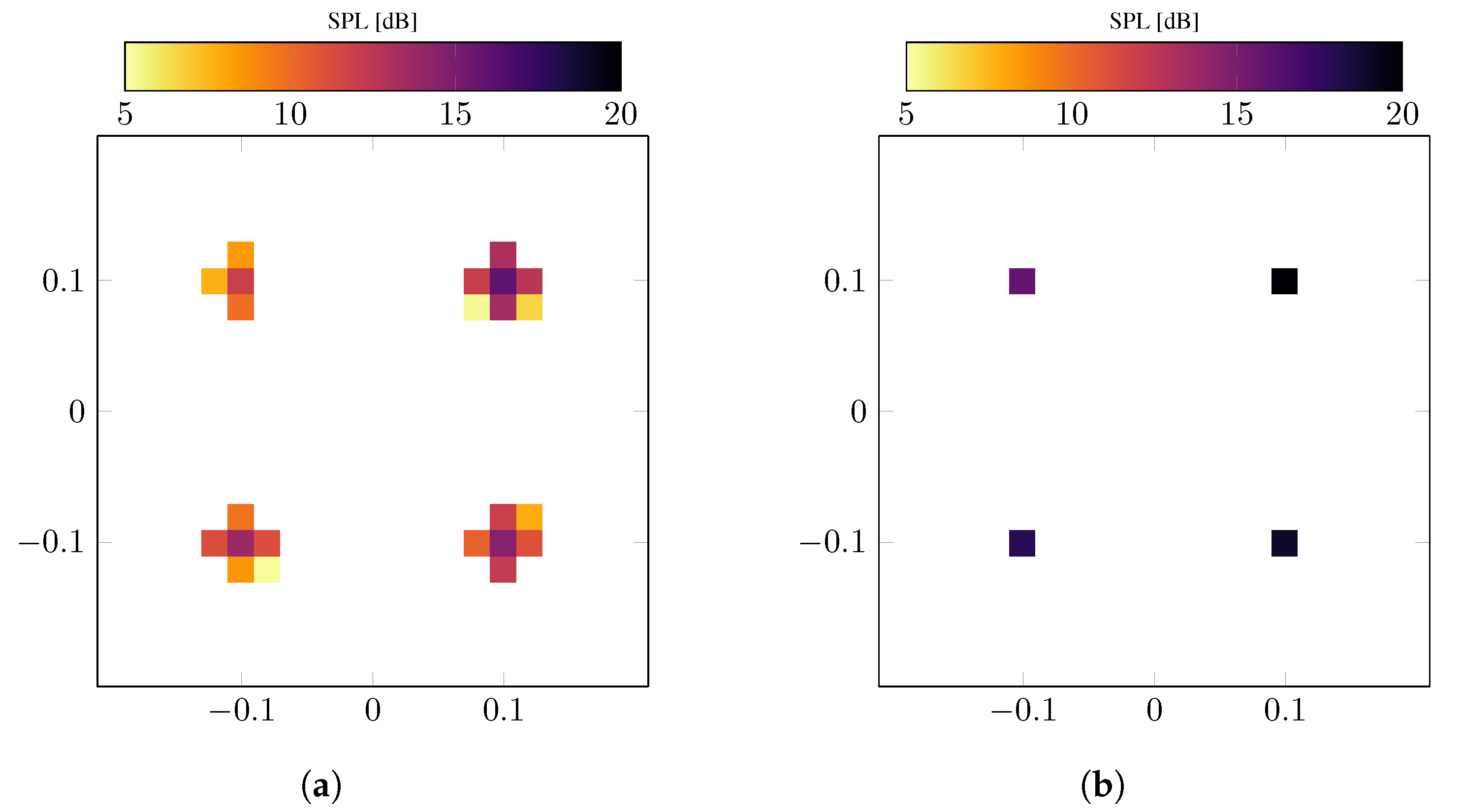
5.2. Random Modeling Error

Secondly, we consider an example with a random perturbation of the phase of the propagation matrix. Such deviations from the true propagation model may occur, e.g., due to small measurement errors of the microphone positions. Recall the definition of the travel times between microphone and source positions (see Equation (2))

$$\Delta t_{mn}=\frac{-({\mathbf{x}}_m-{\mathbf{y}}_n)·\mathbf{m}+{∥{\mathbf{x}}_m-{\mathbf{y}}_n∥}_{\mathbf{m}}}{c{\beta }^2}.$$

By means of the average travel time

$$\overline{\Delta t}=\frac{1}{NM}\sum _{m=1}^M\sum _{n=1}^N\Delta t_{mn},$$

the perturbed phase matrix is defined as

$${\Phi }^{\mathrm{rand}}={\Phi }^{\mathrm{exact}}+(-2\pi f)\sigma \overline{\Delta t}\mathcal{E}.$$

Here, $\mathcal{E}$ is a matrix-valued standard Gaussian random variable and $\sigma$ denotes noise power

$$\mathcal{E}\sim {\left[\mathcal{N}(0,1)\right]}^{M\times N}\sigma =5·{10}^{-3}.$$

The noise power level $\sigma$ is chosen such that

$$\mathbb{E}\left({∥\mathbf{R}\odot exp\left(i{\Phi }^{\mathrm{rand}}\right)-{\mathbf{G}}^{\mathrm{exact}}∥}_F\right)\approx {∥\mathbf{R}\odot exp\left(i{\Phi }^{\mathrm{syst}}\right)-{\mathbf{G}}^{\mathrm{exact}}∥}_F.$$

Hence, the perturbation of the propagation matrix has the same order of magnitude for both noise categories (systematic and random).

Figure 4 shows the reconstruction results for an exemplary realization of the randomly perturbed phase matrix ${\Phi }^{\mathrm{rand}}$ along with the result of the neural network residual minimization (see (11)). In contrast to the systematic error case, the setup is now able to strongly improve the reconstruction result. The final error is of the same order of magnitude as for the FISTA reconstruction with the correct propagation matrix. As this example yields promising results, we consider a small parameter study for three Helmholtz numbers $\mathrm{He}\in \{8,16,32\}$ and $n_{\mathrm{avg}}=100$ random noise realizations each. To evaluate the capabilities of the neural network residual minimization, several statistical measures will be considered.

Firstly, the j-th perturbed phase realization after the n-th gradient step is denoted by

$$\Phi (j,n)\mathrm{for}j=1,\dots ,n_{\mathrm{avg}};n=0,\dots ,n_{\mathrm{grad}}.$$

The cost value (residual) of each individual perturbed phase realization after n gradient descent steps is defined by

$$\cos \mathrm{t}(j,n)=\mathcal{J}\left(\Phi (j,n)\right)j=1,\dots ,n_{\mathrm{avg}};n=0,\dots ,n_{\mathrm{grad}}.$$

Refer to Equation (11) for the definition of the cost function $\mathcal{J}$. The average cost over all noise realizations after n gradient descent steps and the reference cost for the reconstruction with the correct propagation matrix are given by

$$\overline{\cos \mathrm{t}\left(n\right)}=\frac{1}{n_{\mathrm{avg}}}\sum _{j=1}^{n_{\mathrm{avg}}}\cos \mathrm{t}(j,n){\cos \mathrm{t}}_{\mathrm{ref}}=\mathcal{J}\left({\Phi }^{\mathrm{exact}}\right).$$

As a measure of variation among the ensemble, we consider the average positive and negative deviation of cost value measures for each gradient descent step

$$\begin{array}{ccc}\hfill {\cos \mathrm{t}}_{\mathrm{dev}}^{+}\left(n\right)& =& \frac{{\displaystyle \sum _{\cos \mathrm{t}(j,n)\ge \overline{\cos \mathrm{t}\left(n\right)}}}\left|\cos \mathrm{t}(j,n)-\overline{\cos \mathrm{t}\left(n\right)}\right|}{{\displaystyle \sum _{\cos \mathrm{t}(j,n)\ge \overline{\cos \mathrm{t}\left(n\right)}}}1}\hfill \\ \hfill {\cos \mathrm{t}}_{\mathrm{dev}}^{-}\left(n\right)& =& \frac{{\displaystyle \sum _{\cos \mathrm{t}(j,n)<\overline{\cos \mathrm{t}\left(n\right)}}}\left|\cos \mathrm{t}(j,n)-\overline{\cos \mathrm{t}\left(n\right)}\right|}{{\displaystyle \sum _{\cos \mathrm{t}(j,n)<\overline{\cos \mathrm{t}\left(n\right)}}}1}.\hfill \end{array}$$

Similarly, for the reconstruction errors, the source power vector for each noise realization after n gradient descent steps in (11) is denoted by

$$\mathbf{q}(j,n)\mathrm{for}j=1,\dots ,n_{\mathrm{avg}};n=0,\dots ,n_{\mathrm{grad}}$$

and the corresponding error is

$$\mathrm{err}(j,n)={∥\mathbf{q}(j,n)-{\mathbf{q}}^{†}∥}_{2}j=1,\dots ,n_{\mathrm{avg}};n=0,\dots ,n_{\mathrm{grad}}.$$

Again, the average reconstruction error for each gradient descent step and the reference reconstruction error are defined by

$$\overline{\mathrm{err}\left(n\right)}=\frac{1}{n_{\mathrm{avg}}}\sum _{j=1}^{n_{\mathrm{avg}}}\mathrm{err}(j,n){\mathrm{err}}_{\mathrm{ref}}={∥{\mathcal{F}}_{{\Phi }^{\mathrm{exact}}}\left({\mathbf{q}}^{\left(0\right)}\right)-{\mathbf{q}}^{†}∥}_2$$

and the average positive and negative deviations by

$$\begin{array}{ccc}\hfill {\mathrm{err}}_{\mathrm{dev}}^{+}\left(n\right)& =& \frac{{\displaystyle \sum _{\mathrm{err}(j,n)\ge \overline{\mathrm{err}\left(n\right)}}}\left|\mathrm{err}(j,n)-\overline{\mathrm{err}\left(n\right)}\right|}{{\displaystyle \sum _{\mathrm{err}(j,n)\ge \overline{\mathrm{err}\left(n\right)}}}1}\hfill \\ \hfill {\mathrm{err}}_{\mathrm{dev}}^{-}\left(n\right)& =& \frac{{\displaystyle \sum _{\mathrm{err}(j,n)<\overline{\mathrm{err}\left(n\right)}}}\left|\mathrm{err}(j,n)-\overline{\mathrm{err}\left(n\right)}\right|}{{\displaystyle \sum _{\mathrm{err}(j,n)<\overline{\mathrm{err}\left(n\right)}}}1}.\hfill \end{array}$$

Figure 5 shows the previously introduced statistical measures for each gradient descent step and for Helmholtz numbers $\mathrm{He}\in \{8,16,32\}$. For all cases, the mean cost and mean error reach the optimal level of the reference cost and error (dotted line), respectively, after 50–100 gradient descent steps. This shows that for the chosen parameter setup, the method is able to recover solutions of the same error level starting with an erroneous propagation matrix compared to source power reconstruction with the correct propagation matrix. Moreover, the method seems to be robust with respect to additional gradient descent iterations. After the optimal cost and error level are reached, the values stagnate there.

Even though this is still a rather simple synthetic example, the robustness and accuracy of the results with respect to the reconstruction of $\mathbf{q}$ are remarkable. The setup considers $M=64$ microphones, i.e., $\frac{M(M+1)}{2}=2080$ correlation datapoints and $N=441$ focus points. This leads to $M·N=$ 28,224 degrees of freedom (DOFs) for the phase perturbation within the residual minimization. Hence, even for this scenario, problem (11) is heavily underdetermined. Therefore, one should not expect to recover the correct phase matrix ${\Phi }^{\mathrm{exact}}$, at least not in such a setup with much more DOFs than datapoints.

6. Conclusions

In this article, we suggested a framework that accounts for modeling errors in the aeroacoustic source power reconstruction problem. We presented an approach that extends acoustic source power reconstruction based on the FISTA algorithm with additional degrees of freedom (DOFs) that allow a variation of the modeled sound propagation. We restricted our investigations on a variation of the phase of the propagation matrix as this is usually much more affected by the modeling error than the amplitude. Our framework uses the unrolling principle which represents the FISTA optimization by a neural network. The actual optimization with respect to the phase parameters can the be accomplished by standard gradient descent schemes from deep learning. In principle, the neural network representation is not explicitly needed to define the proposed method. However, the great advantage of such a representation is that it leads to a straightforward and efficient implementation using the automatic differentiation abilities of deep learning software packages.

Our results should be seen as a proof of concept for the suggested algorithmic framework. Certainly, this is still work in progress and several more steps are needed to make it usable for experimental data.

The numerical examples show that this approach has the potential to improve source power reconstruction results that are subject to modeling error effects. For random phase perturbations, the algorithm yields very good results in the chosen setup. However, this was a rather friendly setup, where the number of DOFs was approximately 10 times larger than the number of correlation datapoints. For realistic measurement scenarios, this relation becomes even worse. Therefore, in order to move to an application on real experimental datasets, one has to reduce the number of DOFs in the method. Here, we used a brute force strategy where each phase parameter could be varied independently. Alternatively, one may choose a physically motivated parametric phase perturbation model with P parameters, where $P\ll M·N$. The examples with the systematic phase perturbation show that the brute force approach is not well suited if the true perturbation is based on much less DOFs, in this case only one. Further research on this algorithmic approach should examine the performance of the presented framework using parametric perturbations based on the variation of physical parameters such as microphone positions, angle of attack, free stream velocity or speed of sound.

References

1. Billingsley, J.; Kinns, R. The acoustic telescope. J. Sound Vib. 1976, 48, 485–510. [Google Scholar] [CrossRef]
2. Brooks, T.F.; Marcolini, M.A.; Pope, D.S. A directional array approach for the measurement of rotor noise source distributions with controlled spatial resolution. J. Sound Vib. 1987, 112, 192–197. [Google Scholar] [CrossRef]
3. Allen, C.S.; Blake, W.K.; Dougherty, R.P.; Lynch, D.; Soderman, P.T.; Underbrink, J.R. Aeroacoustic Measurements; Springer: Berlin/Heidelberg, Germany, 2002. [Google Scholar] [CrossRef]
4. Oerlemans, S.; Sijtsma, P. Acoustic Array Measurements of a 1:10.6 Scaled Airbus A340 Model. In Proceedings of the 10th AIAA/CEAS Aeroacoustics Conference, Manchester, UK, 10–12 May 2004; American Institute of Aeronautics and Astronautics: Reston, VA, USA, 2004; p. 2924. [Google Scholar] [CrossRef]
5. Soderman, P.; Kafyeke, F.; Boudreau, J.; Burnside, N.; Jaeger, S.; Chandrasekharan, R. Airframe Noise Study of a Bombardier CRJ-700 Aircraft Model in the NASA Ames 7-by 10-Foot Wind Tunnel. Int. J. Aeroacoustics 2004, 3, 1–42. [Google Scholar] [CrossRef]
6. Johnson, D.H.; Dudgeon, D.E. Array Signal Processing; P T R Prentice Hall: Englewood Cliffs, NJ, USA, 1993. [Google Scholar]
7. Sijtsma, P. CLEAN Based on Spatial Source Coherence. Int. J. Aeroacoustics 2007, 6, 357–374. [Google Scholar] [CrossRef]
8. Brooks, T.F.; Humphreys, W.M. A deconvolution approach for the mapping of acoustic sources (DAMAS) determined from phased microphone arrays. J. Sound Vib. 2006, 294, 856–879. [Google Scholar] [CrossRef]
9. Blacodon, D.; Elias, G. Level Estimation of Extended Acoustic Sources Using a Parametric Method. J. Aircraft 2004, 41, 1360–1369. [Google Scholar] [CrossRef]
10. Yardibi, T.; Li, J.; Stoica, P.; Cattafesta, L.N. Sparsity constrained deconvolution approaches for acoustic source mapping. J. Acoust. Soc. Am. 2008, 123, 2631–2642. [Google Scholar] [CrossRef]
11. Beck, A.; Teboulle, M. A Fast Iterative Shrinkage-Thresholding Algorithm for Linear Inverse Problems. SIAM J. Imaging Sci. 2009, 2, 183–202. [Google Scholar] [CrossRef] [Green Version]
12. Chambolle, A.; Vore, R.D.; Lee, N.Y.; Lucier, B. Nonlinear wavelet image processing: Variational problems, compression, and noise removal through wavelet shrinkage. IEEE Trans. Image Process. 1998, 7, 319–335. [Google Scholar] [CrossRef]
13. Daubechies, I.; Defrise, M.; Mol, C.D. An iterative thresholding algorithm for linear inverse problems with a sparsity constraint. Commun. Pure Appl. Math. 2004, 57, 1413–1457. [Google Scholar] [CrossRef]
14. Chen, L.; Xiao, Y.; Yang, T. Application of the improved fast iterative shrinkage-thresholding algorithms in sound source localization. Appl. Acoust. 2021, 180, 108101. [Google Scholar] [CrossRef]
15. Lylloff, O.; Fernández-Grande, E.; Agerkvist, F.; Hald, J.; Tiana-Roig, E.; Andersen, M.S. Improving the efficiency of deconvolution algorithms for sound source localization. J. Acoust. Soc. Am. 2015, 138, 172–180. [Google Scholar] [CrossRef] [PubMed]
16. Shen, L.; Chu, Z.; Yang, Y.; Wang, G. Periodic boundary based FFT-FISTA for sound source identification. Appl. Acoust. 2018, 130, 87–91. [Google Scholar] [CrossRef]
17. Shen, L.; Chu, Z.; Tan, L.; Chen, D.; Ye, F. Improving the Sound Source Identification Performance of Sparsity Constrained Deconvolution Beamforming Utilizing SFISTA. Shock Vib. 2020, 2020, 1482812. [Google Scholar] [CrossRef]
18. Monga, V.; Li, Y.; Eldar, Y.C. Algorithm Unrolling: Interpretable, Efficient Deep Learning for Signal and Image Processing. IEEE Signal Process. Mag. 2021, 38, 18–44. [Google Scholar] [CrossRef]
19. Castellini, P.; Giulietti, N.; Falcionelli, N.; Dragoni, A.F.; Chiariotti, P. A neural network based microphone array approach to grid-less noise source localization. Appl. Acoust. 2021, 177, 107947. [Google Scholar] [CrossRef]
20. Lee, S.Y.; Chang, J.; Lee, S. Deep learning-based method for multiple sound source localization with high resolution and accuracy. Mech. Syst. Signal Process. 2021, 161, 107959. [Google Scholar] [CrossRef]
21. Lee, S.Y.; Chang, J.; Lee, S. Deep Learning-Enabled High-Resolution and Fast Sound Source Localization in Spherical Microphone Array System. IEEE Trans. Instrum. Meas. 2022, 71, 1–12. [Google Scholar] [CrossRef]
22. Ma, W.; Liu, X. Phased microphone array for sound source localization with deep learning. Aerosp. Syst. 2019, 2, 71–81. [Google Scholar] [CrossRef]
23. Mukherjee, S.; Dittmer, S.; Shumaylov, Z.; Lunz, S.; Öktem, O.; Schönlieb, C.B. Learned Convex Regularizers for Inverse Problems. arXiv 2020, arXiv:2008.02839. [Google Scholar]
24. Li, H.; Schwab, J.; Antholzer, S.; Haltmeier, M. NETT: Solving inverse problems with deep neural networks. Inverse Probl. 2020, 36, 065005. [Google Scholar] [CrossRef]
25. Lunz, S.; Hauptmann, A.; Tarvainen, T.; Schönlieb, C.B.; Arridge, S. On Learned Operator Correction in Inverse Problems. SIAM J. Imaging Sci. 2021, 14, 92–127. [Google Scholar] [CrossRef]
26. Borgerding, M.; Schniter, P.; Rangan, S. AMP-Inspired Deep Networks for Sparse Linear Inverse Problems. IEEE Trans. Signal Process. 2017, 65, 4293–4308. [Google Scholar] [CrossRef]
27. Gregor, K.; LeCun, Y. Learning fast approximations of sparse coding. In Proceedings of the ICML 2010—Proceedings, 27th International Conference on Machine Learning, Haifa, Israel, 21–24 June 2010; pp. 399–406. [Google Scholar]
28. Ito, D.; Takabe, S.; Wadayama, T. Trainable ISTA for Sparse Signal Recovery. IEEE Trans. Signal Process. 2019, 67, 3113–3125. [Google Scholar] [CrossRef]
29. Takabe, S.; Wadayama, T.; Eldar, Y.C. Complex Trainable Ista for Linear and Nonlinear Inverse Problems. In Proceedings of the ICASSP 2020—2020 IEEE International Conference on Acoustics, Speech and Signal Processing (ICASSP), Barcelona, Spain, 4–8 May 2020; pp. 5020–5024. [Google Scholar] [CrossRef]
30. Kayser, C.; Kujawski, A.; Sarradj, E. A trainable iterative soft thresholding algorithm for microphone array source mapping. In Proceedings of the CD of the 9th Berlin Beamforming Conference, Berlin, Germany, 8–9 June 2022; pp. 1–17. [Google Scholar]
31. Golub, G.H.; Hansen, P.C.; O’Leary, D.P. Tikhonov Regularization and Total Least Squares. SIAM J. Matrix Anal. Appl. 1999, 21, 185–194. [Google Scholar] [CrossRef]
32. Kluth, T.; Maass, P. Model uncertainty in magnetic particle imaging: Nonlinear problem formulation and model-based sparse reconstruction. Int. J. Magn. Part. Imaging 2017, 3, 1707004. [Google Scholar] [CrossRef]
33. Dittmer, S.; Kluth, T.; Maass, P.; Baguer, D.O. Regularization by Architecture: A Deep Prior Approach for Inverse Problems. J. Math. Imaging Vis. 2019, 62, 456–470. [Google Scholar] [CrossRef]
34. Beck, A. First-Order Methods in Optimization; Society for Industrial and Applied Mathematics: Philadelphia, PA, USA, 2017. [Google Scholar] [CrossRef] [Green Version]
35. Chardon, G.; Picheral, J.; Ollivier, F. Theoretical analysis of the DAMAS algorithm and efficient implementation of the covariance matrix fitting method for large-scale problems. J. Sound Vib. 2021, 508, 116208. [Google Scholar] [CrossRef]
36. Engl, H.W.; Hanke, M.; Neubauer, A. Regularization of Inverse Problems; Springer: Dordrecht, The Netherlands, 1996. [Google Scholar]
37. Kingma, D.P.; Ba, J. Adam: A method for stochastic optimization. arXiv 2014, arXiv:1412.6980. [Google Scholar]
38. Sarradj, E.; Herold, G.; Sijtsma, P.; Martinez, R.M.; Geyer, T.F.; Bahr, C.J.; Porteous, R.; Moreau, D.; Doolan, C.J. A Microphone Array Method Benchmarking Exercise using Synthesized Input Data. In Proceedings of the 23rd AIAA/CEAS Aeroacoustics Conference. American Institute of Aeronautics and Astronautics, Denver, CO, USA, 5–9 June 2017; p. 3719. [Google Scholar] [CrossRef] [Green Version]
39. Abadi, M.; Agarwal, A.; Barham, P.; Brevdo, E.; Chen, Z.; Citro, C.; Corrado, G.S.; Davis, A.; Dean, J.; Devin, M.; et al. TensorFlow: Large-Scale Machine Learning on Heterogeneous Systems. 2015. Available online: https://www.tensorflow.org/ (accessed on 24 August 2022).
40. Géron, A. Hands-on Machine Learning with Scikit-Learn, Keras, and TensorFlow; O’Reilly Media: Sebastopol, CA, USA, 2019. [Google Scholar]
Figure 1. Sketch of the unrolled FISTA network F . One forward pass through the network is equivalent to the application of n iter FISTA iterations. Green bounding boxes indicate one iteration of the FISTA algorithm, trainable parameters are marked in blue.
Acoustics 04 00050 g001
Figure 2. Reference solutions for numerical example. (a) Exact solution; (b) FISTA solution with exact phase ( q q 2 = 7.49 ).
Acoustics 04 00050 g002
Figure 3. Solutions for numerical example with systematic phase perturbation. (a) FISTA solution with perturbed phase ( q q 2 = 106.61 ); (b) FISTA solution after phase error compensation ( q q 2 = 104.46 ).
Acoustics 04 00050 g003
Figure 4. Solutions for numerical example with random phase perturbation. (a) FISTA solution with perturbed phase ( q q 2 = 106.31 ); (b) FISTA solution after phase error compensation ( q q 2 = 6.56 ).
Acoustics 04 00050 g004
Figure 5. Cost and error graphs for several Helmholtz numbers. The colored area indicates the interval cos t ( n ) ¯ ± 2 cos t dev ± ( n ) and err ( n ) ¯ ± 2 err dev ± ( n ) .
Acoustics 04 00050 g005