One-Way Wave Equation Derived from Impedance Theorem

Abstract

The wave equations for longitudinal and transverse waves being used in seismic calculations are based on the classical force/moment balance. Mathematically, these equations are 2nd order partial differential equations (PDE) and contain two solutions with a forward and a backward propagating wave, therefore also called “Two-way wave equation”. In order to solve this inherent ambiguity many auxiliary equations were developed being summarized under “One-way wave equation”. In this article the impedance theorem is interpreted as a wave equation with a unique solution. This 1st order PDE is mathematically more convenient than the 2nd order PDE. Furthermore the 1st order wave equation being valid for three-dimensional wave propagation in an inhomogeneous continuum is derived.

1. Introduction

The n-th order differential equation has n linearly independent solutions. In the classical 2nd order wave equation with n = 2, the solutions are the two waves running in forward and backward direction. Hence, the common term in seismic contexts is “Two-way wave equation”. For analytical calculations, by choosing the root of c² as +c or –c, the relevant wave direction needs to be selected. Due to the obvious ambiguity, a factorization [1] of the 2nd order partial differential equation (PDE) into two 1st order PDEs has been known (but not further applied) by seismicians for many decades:

$$\left(\frac{{\partial }^2}{\partial {\mathrm{t}}^2}-{\mathrm{c}}^2\frac{{\partial }^2}{\partial {\mathrm{x}}^2}\right)\mathrm{s}=\left(\frac{\partial }{\partial \mathrm{t}}-\mathrm{c}\frac{\partial }{\partial \mathrm{x}}\right)\left(\frac{\partial }{\partial \mathrm{t}}+\mathrm{c}\frac{\partial }{\partial \mathrm{x}}\right)\mathrm{s}=0$$

(1)

From this attempt two One-way wave equations result, but the original Equation (1) is only valid for straight wave propagation in a homogeneous continuum. Therefore for the calculation of three- dimensional wave propagation in an inhomogeneous continuum a huge number of additional equations were developed being summarized under the title “One-way wave equation”. A recent approach uses anti–sound techniques to extinguish backward travelling disturbing waves [2].

Corresponding to the great economic importance of seismic prospecting, the issue of “One/Two-way wave equation” is supplemented by a comprehensive amount of patents in addition to the relevant literature. In the absence of review articles, [3] and [4] are listed, that contain long lists of references. The multitude of solution trials of the last decades and the recent years are an obvious indication for a still unsatisfactory situation.

2. Method

The impedance theorem was introduced in 1886 by Heaviside. Originally written for electrodynamics, the concept was taken over by acoustics and has become an indispensable tool in seismology as well. Identical to the impedance formula is the so-called “Ohm’s acoustic law”.

In this article the impedance theorem is directly (i.e., unadulterated and hypothesis-free) transformed into an exact “One-way wave equation” being valid for longitudinal wave propagation. By taking a homogeneous solid with straight wave propagation as a starting point, also for an inhomogeneous solid the curved wave propagation in three-dimensional space is derived.

3. One-Way Wave Equation: Longitudinal Wave Propagation in a Homogenous Continuum

A lossless, isotropic and homogeneous continuum with density ρ [kg/m³] and elastic modulus E [Pa] has the longitudinal wave velocity c [m/s] and the specific impedance z = ρ c [kg/m²s = sPa/m]

$$\mathrm{c}=\sqrt{\mathrm{E}/\mathsf{\rho }}$$

(2)

$$\mathrm{z}=\mathsf{\rho }\mathrm{c}=\sqrt{\mathrm{E}\mathsf{\rho }}$$

(3)

In a longitudinal plane wave, the impedance determines the local proportionality of sound pressure p = p(x,t) [Pa] and particle velocity v = v(x,t) [m/s].

$$\frac{\mathrm{p}}{\mathrm{v}}=\mathsf{\rho }\mathrm{c}$$

(4)

For simplicity only the loss-free case is considered. With a complex elastic modulus damped wave propagation can be calculated. The conversion of the impedance equation used in the formula

ρ c v − p = 0

(5)

is known as “Ohm’s acoustic law” (

Table 1. Impedance theorem and Ohm’s law in electricity and acoustics.

	Electricity	Acoustics
Resistance	R [V/A]	z = ρ c [sPa/m]
Current	I [A]	v = $\dot{\mathrm{s}}$ [m/s]
Voltage	U [V]	p = E s′ [Pa]
Impedance-Theorem	R = U/ I	ρ c = p/v
Ohm’s law	R I − U = 0	ρ c v − p = 0

). An electrical voltage U in a conductor with resistance R causes the current flow I = U/R. In analogy, a local sound pressure p at the impedance z = ρc induces a local particle velocity v = $\dot{\mathrm{s}}$ = p/ρc (with displacement s, v = $\dot{\mathrm{s}}$ = ∂s/∂t, $\ddot{\mathrm{s}}$ = ∂²s/∂t², s′= ∂s/∂x).

A longitudinal plane wave of frequency ω (rad/s) and with displacement amplitude a [m] has the displacement s = s(x,t) [m] Equation (6), the particle velocity v Equation (7) and the pressure p Equation (8). For the respective equations, it is useful to combine, with agreement in Equation (9), the individual independent waves in the forward and the backward directions within one formula:

$$\mathrm{s}=\mathrm{s}(\mathrm{x},\mathrm{t})=\mathrm{a}\sin \left(\mathsf{\omega }\left(\mathrm{t}-\frac{\mathrm{x}}{\mathrm{c}}\right)\right)$$

(6)

$$\mathrm{v}=\frac{\partial \mathrm{s}}{\partial \mathrm{t}}=\dot{\mathrm{s}}=\mathrm{a}\mathsf{\omega }\cos \left(\mathsf{\omega }\left(\mathrm{t}-\frac{\mathrm{x}}{\mathrm{c}}\right)\right)$$

(7)

$$\mathrm{p}:=\mathrm{E}\frac{\partial \mathrm{s}}{\partial \mathrm{x}}=\mathrm{E}{\mathrm{s}}^{\prime }=-(\mathrm{E}\mathrm{a}\mathsf{\omega }/\mathrm{c})\cos \left(\mathsf{\omega }\left(\mathrm{t}-\frac{\mathrm{x}}{\mathrm{c}}\right)\right)$$

(8)

c = {+c, −c}  a = {a₊, a₋}

(9)

These relations, with the identity E = ρ c² in Equation (2) being inserted into impedance Equation (5), result in a 1st order PDE as longitudinal wave equation for the homogeneous medium

$$\dot{\mathrm{s}}-\mathrm{c}{\mathrm{s}}^{\prime }=0\hspace{1em}\hspace{1em}\mathrm{c}=\{+\mathrm{c},-\mathrm{c}\}$$

(10)

that competes with the conventional 2nd order PDE for the homogeneous longitudinal waveguide

$$\ddot{\mathrm{s}}-{\mathrm{c}}^2{\mathrm{s}}^{″}=0$$

(11)

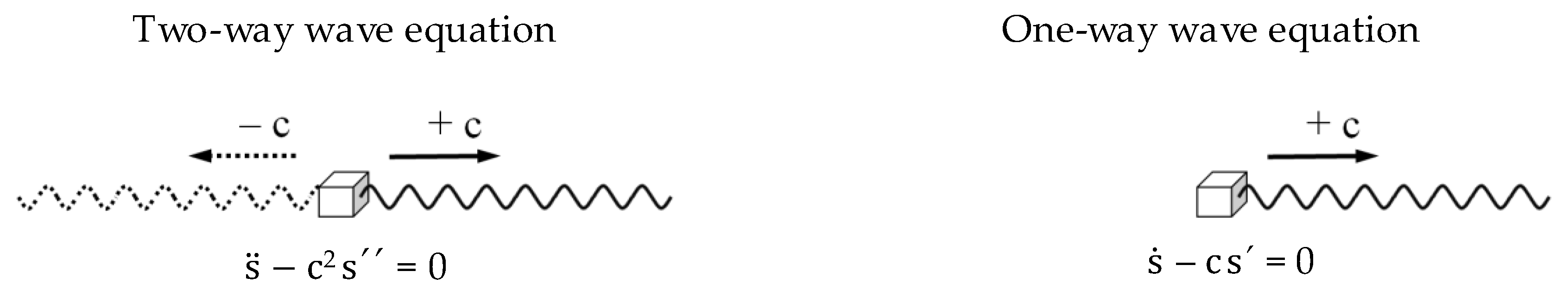
As can be verified, both PDEs provide the identical longitudinal propagating wave as seen in Equation (6). The difference is that for 1st order PDE (10) the wave direction +c or −c is set with respect to the task at the start of the calculation and a unique solution is obtained (Figure 1). On the other hand, the 2nd order PDE (2) includes both the forward and the backward traveling waves due to c² = (+c)² = (−c)² and the standing wave solution (φ = arbitrary phase angle)

$$\mathrm{s}={\mathrm{a}}_{+/-}\sin \left(\mathsf{\omega }\mathrm{t}\right)\sin \left(\mathsf{\omega }\frac{\mathrm{x}}{\mathrm{c}}+\mathsf{\phi }\right)$$

(12)

Therefore, in the numerical finite element calculation, it is yet necessary to additionally use auxiliary One-way wave equations for selecting the relevant wave direction or for eliminating unwanted wave portions.

4. One-Way Wave Equation: Longitudinal Wave Propagation in an Inhomogeneous Continuum

An inhomogeneous continuum is described by the global coordinates x = {xi, yj, zk}. In a field point ʘ = ʘ(x) the location-dependent material parameters ρ = ρ(x) and E = E(x) exist. In accordance with the locality axiom, the wave velocity c(x) is also location-dependent

$$\mathrm{c}(\mathbf{x})=\sqrt{\frac{\mathrm{E}(\mathbf{x})}{\mathsf{\rho }\left(\mathbf{x}\right)}}$$

(13)

With respect to linear theory a continuous inhomogeneity is assumed (λ[m] = wave length):

λ∇E << E  λ∇ρ << ρ

(14)

In case of inhomogeneity, waves do not propagate in a straight way. Generalizing to curved waves, in addition to the global coordinates x, the local coordinates {ξt, n, b} of the accompanying tripod being located in the respective field point ʘ are introduced (t, n, b: orthogonal unit vectors; ξ[m]: coordinate in t-direction).

$$\mathbf{t}=\mathbf{t}(\mathbf{x},\mathrm{t})=\frac{\mathbf{c}}{\mathrm{c}}\hspace{1em}\hspace{1em}\mathbf{t}·\mathbf{t}=1$$

(15)

$$\mathbf{n}=\mathbf{n}(\mathbf{x},\mathrm{t})=\frac{\mathbf{t}·\nabla \mathbf{t}}{|\mathbf{t}·\nabla \mathbf{t}|}=\mathrm{R}\mathbf{R}{}^{-1}$$

(16)

b = t × n

(17)

The tangential vector t points in the wave direction c (since t is only used as vector it can be distinguished from scalar time t). In the Frenet theory for space curves, a change of direction ∇t corresponds to a curvature radius R [m]

$$\mathbf{t}·\nabla \mathbf{t}=-\mathbf{t}\times \mathrm{rot}\mathbf{t}=\frac{1}{R}=\frac{n}{\mathrm{R}}$$

(18)

The vectorial curvature radius R = Rn determines the normal direction n. The local wave propagation takes place in the so-called osculating plane being spanned by the tangential vector t and the normal vector n, whereby the vertical binormal vector b direction is force-free. The relevant field parameters are the linear elastic vector displacement s = s(x,t) [m], the velocity $\dot{s}$ = v = ∂s/∂t [m/s], the gradient ∇s [–] and the pressure p = ∇Es [Pa] measured at fixed coordinate x and time t [s]. Together with the vectorial impedance z = ρc = ρct inserted into the basic Equation (5) the constitutive tensor Equation (19) for the inhomogeneous medium follows. By scalar multiplication with c = ct the tensor Equation (19) can be transformed into the vector form in Equation (20)

$$\mathsf{\rho }\mathbf{c}\dot{\mathbf{s}}-\nabla \left(\mathrm{E}\mathbf{s}\right)=\mathbf{0}$$

(19)

$$\mathsf{\rho }{\mathrm{c}}^2\dot{\mathbf{s}}-\mathbf{c}·\nabla \left(\mathrm{E}\mathbf{s}\right)=\mathbf{0}$$

(20)

For longitudinal wave propagation, per definition, the displacement s points into the t-direction, i.e.,

s = s t

(21)

$$\dot{\mathbf{s}}=\partial \left(\mathrm{s}\mathbf{t}\right)/\partial \mathrm{t}=\dot{\mathrm{s}}\mathbf{t}+\mathrm{s}\dot{\mathbf{t}}=\dot{\mathrm{s}}\mathbf{t}+\mathrm{s}\left|\dot{\mathbf{t}}\right|\mathbf{n}$$

(22)

$$\nabla \mathbf{s}=\nabla \left(\mathrm{s}\mathbf{t}\right)=(\nabla \mathrm{s})\mathbf{t}+\mathrm{s}\nabla \mathbf{t}$$

(23)

These expressions inserted in Equation (20) lead to the vector equation with t- and n-components (∇E/E = ∇(ln E)):

$$(\dot{\mathrm{s}}\mathbf{t}+\mathrm{s}\dot{\mathbf{t}})-\mathrm{c}\mathbf{t}·(\mathrm{s}\mathbf{t}·\nabla (\ln \mathrm{E})+(\nabla \mathrm{s})\mathbf{t}+\mathrm{s}\nabla \mathbf{t})=\mathbf{0}$$

(24)

$$\mathbf{t}-\mathrm{components}:\hspace{1em}\hspace{1em}\mathbf{t}(\dot{\mathrm{s}}-\mathrm{c}\mathbf{t}·\nabla \left(\ln \mathrm{E}\right)+\mathrm{c}\mathbf{t}·\nabla \mathrm{s})=\mathbf{0}$$

(25)

$$\mathbf{n}-\mathrm{components}:\hspace{1em}\hspace{1em}\mathrm{s}\dot{\mathbf{t}}-\mathrm{sc}\mathbf{t}·\nabla \mathbf{t}=\mathbf{0}\hspace{1em}\to \hspace{1em}\dot{\mathbf{t}}-\mathrm{c}\mathbf{n}/\mathrm{R}=\mathbf{0}$$

(26)

The t-components in Equation (25) refer to the equilibrium in t-direction. With the identities

$$\mathbf{t}·\nabla \mathrm{s}=\frac{\partial \mathrm{s}}{\partial \mathsf{\xi }}:={\mathrm{s}}^{`}$$

(27)

$$\mathbf{t}·\nabla (\ln \mathrm{E}):={\left(\ln \mathrm{E}\right)}^{`}$$

(28)

results the scalar wave equation as a function of coordinate ξ [m] running in wave direction t = t(x)

$$\dot{\mathrm{s}}-\mathrm{c}({\left(\ln \mathrm{E}\right)}^{`}\mathrm{s}+{\mathrm{s}}^{`})=0$$

(29)

By inserting the particle velocity $\dot{\mathrm{s}}$ = iωs and s`/s = (lns)` in Equation (29)

iω/c − (lnE)` + (lns)` = 0

(30)

the solution in the ξt-tripod-coordinate follows, sic:

$$\mathrm{s}={\mathrm{s}}_{\mathrm{0}}\frac{{\mathrm{E}}_{\mathrm{o}}}{\mathrm{E}}\exp (\mathrm{i}\mathsf{\omega }(\mathrm{t}-{{\displaystyle \int }}_0^{\mathsf{\xi }}\frac{\mathrm{d}\mathsf{\xi }}{\mathrm{c}}))$$

(31)

For the specific case of a constant wave velocity c = const. the integral simplifies to ${{\displaystyle \int }}_0^{\mathsf{\xi }}\frac{\mathrm{d}\mathsf{\xi }}{\mathrm{c}}$ = $\mathsf{\xi }/\mathrm{c}$.

The n-component in Equation (26) refers to the tautological relationship of a circular motion with radius R [m], circumferential wave velocity c and angular velocity |$\dot{\mathbf{t}}$| [rad/s]

$$|\dot{t}|=\frac{\mathrm{c}}{\mathrm{R}}$$

(32)

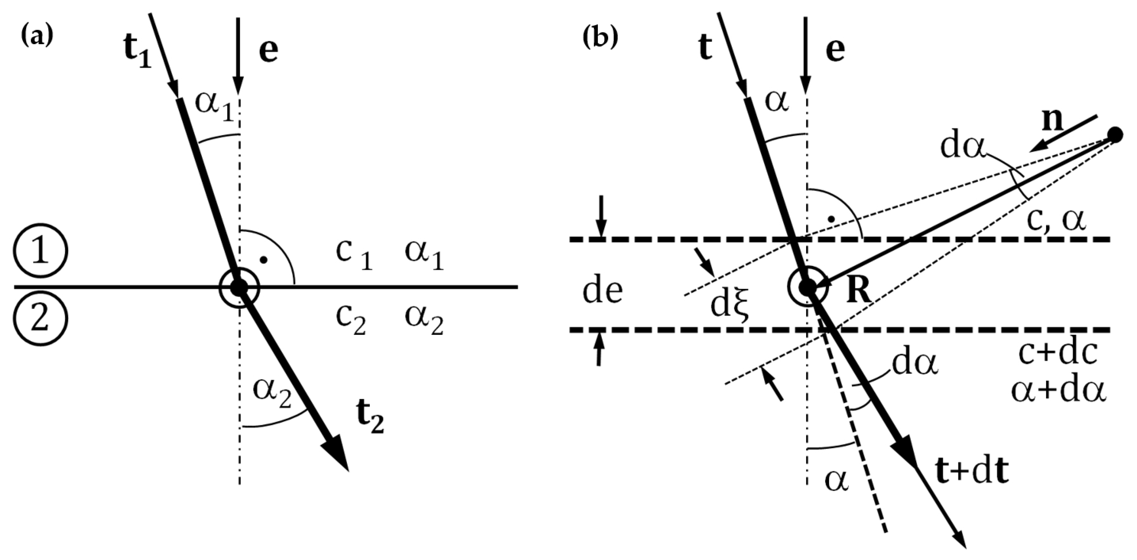
With reference to the differential time interval dt, the angle change dα = |$\dot{\mathbf{t}}$| dt corresponds to a displacement change dξ = c dt in circumferential direction and following relation (Figure 2a) results:

$$\mathrm{R}=\frac{\mathrm{d}\mathsf{\xi }}{\mathrm{d}\mathsf{\alpha }}$$

(33)

The curvature radius R of the wave is determined by Snell’s law:

$$\frac{\sin {\mathsf{\alpha }}_1}{{\mathrm{c}}_1}=\frac{\sin {\mathsf{\alpha }}_2}{{\mathrm{c}}_2}=\frac{\sin \mathsf{\alpha }}{\mathrm{c}}=\mathrm{const}.$$

(34)

At the interface boundary plane of two waveguides with different wave velocities c₁ und c₂, the angle of incidence α₁ being measured from perpendicular direction e changes to α₂ (Figure 2a).

The wave form in an inhomogeneous medium (Figure 2b) is similar, but the velocity step c₁ → c₂ is replaced by an infinitesimal differential dc. The perpendicular vector e is determined by the local velocity gradient ∇c in the field point ʘ

$$\mathbf{e}=\mathbf{e}(\mathbf{x})=\frac{\nabla \mathrm{c}}{|\nabla \mathrm{c}|}$$

(35)

In a layer vertical to e with the differential thickness de the velocity difference dc is given by

$$\mathrm{dc}=\mathrm{de}|\nabla \mathrm{c}|$$

(36)

According to the differential Snell’s law

$$\frac{\sin \mathsf{\alpha }}{\mathrm{c}}=\frac{\sin \left(\mathsf{\alpha }+\mathrm{d}\mathsf{\alpha }\right)}{\mathrm{c}+\mathrm{dc}}=\mathrm{const}.$$

(37)

the differential dc at an angle of incidence α refers to the angle differential dα (Figure 2b)

$$\mathrm{d}\mathsf{\alpha }=\tan \mathsf{\alpha }\frac{\mathrm{dc}}{\mathrm{c}}=\tan \mathsf{\alpha }\frac{|\nabla \mathrm{c}|}{\mathrm{c}}\mathrm{de}$$

(38)

Within the layer de the sound beam covers the distance dξ

$$\mathrm{d}\mathsf{\xi }=\frac{\mathrm{de}}{\cos \mathsf{\alpha }}$$

(39)

In accordance with Equation (33), a directional change dα along a path dξ corresponds to the curvature radius R = dξ/dα. Thus, a wave from direction α at the field point ʘ is bent − due to the local gradient ∇c − according to the local curvature radius R

$$\mathrm{R}=\frac{\mathrm{c}}{|\nabla \mathrm{c}|\sin \mathsf{\alpha }}$$

(40)

Knowing the wave curvature allows larger increments in finite element calculations and is also useful for ray tracing.

5. Results

The impedance theorem is equivalent with a 1st order PDE that can be interpreted as a One-way wave equation for one-dimensional wave propagation. For an inhomogeneous continuum, a vectorial form of the One-way wave equation has been derived using Snell’s law (

Table 2. Derivation of the One-way wave equation from impedance theorem, overview of results.

	One-Way Wave Equations Derived from Impedance Theorem
Derivation	a) ρc v − p = 0 Impedance Theorem (Ohm’s acoustic law) b) v = $\frac{\partial \mathrm{s}}{\partial \mathrm{t}}$ = $\dot{\mathrm{s}}$ and p = E $\frac{\partial \mathrm{s}}{\partial \mathrm{x}}$ = E s′ Note: Derivation also possible with impulse flow equilibrium [5,6,7].
1D wave propagation, homogeneous continuum	$\dot{\mathrm{s}}$ −c s′= 0  with c = {+c, −c} and c = $\sqrt{\mathrm{E}/\mathsf{\rho }}$ s = a sin $\left(\mathsf{\omega }\left(\mathrm{t}-\frac{\mathrm{x}}{\mathrm{c}}\right)\right)$
3D wave propagation, inhomogeneous continuum	ρc$\dot{s}$− ∇(Es) = 0 with c = {+ c, – c} and c($x$) = $\sqrt{\mathrm{E}\left(x\right)/\mathsf{\rho }\left(x\right)}$ s = s0 $\frac{E_o}{E}$ exp $\left(\mathrm{i}\mathsf{\omega }\left(t-{{\displaystyle \int }}_0^{\mathsf{\xi }}\frac{\mathrm{d}\mathsf{\xi }}{\mathrm{c}}\right)\right)$

). In addition, the wave curvature in an inhomogeneous continuum could be found. Interestingly, the vectorial One-way wave equation also results from the hypothetical impulse flow equilibrium [4,5,6].

6. Discussion

The One-way wave equations and the Two-way wave equations show significant differences. For a better comparison, the 1st order PDE / One-way Equation (10) and the 2nd order PDE / Two-way Equation (11) for the homogeneous waveguide are rewritten in the quotient form

$$\dot{\mathrm{s}}/{\mathrm{s}}^{\prime }=\mathrm{c}$$

(41)

$$\ddot{\mathrm{s}}/{\mathrm{s}}^{″}={\mathrm{c}}^2$$

(42)

In the One-way wave Equation (41), the particle velocity $\dot{\mathrm{s}}$ [m/s] and the gradient s′ [–] are the field variables. Their quotient provides the speed of sound c = {+c, −c} defining the wave direction. The solution of the 1st order One-way wave equation is obtained by simple one-time integration.

However, the Two-way wave Equation (42) is based on the field variable‘s acceleration $\ddot{\mathrm{s}}$ [m/s²] and the displacement‘s double gradient s″ [1/m]. It is significant that their quotient with the ambiguous result c² = (+c)² = (−c)² does not contain information regarding the direction of the wave. The higher level of differentiation of these variables also results in higher mathematical efforts for solving the 2nd order Two-way wave equation.

7. Conclusions

The One-way wave Equation (19) has been derived from the elementary impedance theorem. The One-way wave equations show lower differentiation levels and are more convenient to use then the Two-way wave equations with their 2nd order derivatives. The One-way wave Equation (19) for three-dimensional wave propagation in an inhomogeneous continuum and its solution (31) could potentially enhance seismic calculations as well as finite elements methods [8,9].

References

1. Baysal, E.; Kosloff, D.D.; Sherwood, J.W.C. A two-way nonreflecting wave equation. Geophysics 1984, 49, 132–141. [Google Scholar] [CrossRef] [Green Version]
2. Maeda, K.; Colonius, T. A source term approach for generation of one-way acoustic waves in the Euler and Navier-Stokes equation. Wave Motion 2017, 75, 36–49. [Google Scholar] [CrossRef] [PubMed] [Green Version]
3. Angus, D.A. The One-Way Wave Equation: A Full-Waveform Tool for Modeling Seismic Body Wave Phenomena. Surv. Geophys. 2014, 35, 359–393. [Google Scholar] [CrossRef] [Green Version]
4. Luo, M.; Jin, S. Halliburton Energy Services: Hybrid One-Way and Full-Way Wave Equation Migration. US-Patent US8116168, 14 February 2012. [Google Scholar]
5. Bschorr, O. Deviationswellen im Festkörper [Deviation waves in solids]. In Proceedings of the DAGA 2014—40th German Annual Conference of Acoustics, Oldenburg, Germany, 10–13 March 2014; pp. 80–81. [Google Scholar]
6. Bschorr, O. Wellen im anisotropen Festkörper nach dem Impulskonzept [Waves in anisotropic solids according to the impulse concept]. In Proceedings of the DAGA 2016—42th German Annual Conference of Acoustics, Aachen, Germany, 14–17 March 2016; pp. 270–271. [Google Scholar]
7. Raida, H.-J.; Bschorr, O. Konventionelles Kräftegleichgewicht versus hypothetisches Impulsgleichgewicht [Conventional force equilibrium versus hypothethical impulse equilibrium]. In Proceedings of the DAGA 2018—44th German Annual Conference of Acoustics, Aachen, Germany, 19–22 March 2018; pp. 828–831. [Google Scholar]
8. Bschorr, O. Verfahren zur Berechnung von Schwingungen in Kontinuen [Procedure for calculating vibrations in continuums]. German Patent Application DE102014019643A1, 31 December 2014. [Google Scholar]
9. Bschorr, O. Verfahren zur Berechnung von elastischen Festkörpern [Procedure for the calculation of elastic solids]. German Patent Application DE102016005236A1, 29 April 2016. [Google Scholar]
Figure 1. 1D-waveguide with sinusoidal wave propagation (single waveguide element is displayed): Two-way wave equation with two solutions according to the wave velocities +c and –c vs. One-way wave equation with one unique solution acc. to the chosen wave velocity c (here: +c).
Acoustics 02 00012 g001
Figure 2. (a) A sound wave from direction t at the interface boundary plane of two homogeneous media (1 and 2) with different wave velocities c1 and c2 (here: c2 > c1) is refracted from the angle α1 to α2 according to Snell’s Law (34). The vector e is perpendicular to the interface. (b) A sound wave from direction t propagates through an inhomogeneous medium. The osculation plane is defined by tangential vector t and normal vector n lying within the drawing plane. In a field point ʘ the velocity gradient ∇c determines the perpendicular direction e = ∇c / | c | . The angle differential dα results from the differential Snell’s Law in Equation (37).
Acoustics 02 00012 g002