Positive Position Feedback Control of a Galloping Structure

Abstract

In this study, the suppression of wind-induced oscillations of a D-shaped prism mounted on a cantilever beam by means of a positive position feedback (PPF) controller is investigated. The assumed mode method is applied to determine the stiffness, mass and non-linear force matrixes of a second order ordinary differential equation system. The positive position feedback control by use of a sensor-actuator piezoelectric is implemented on the galloping system to suppress the mechanical oscillations. The results show that the PPF controller is a powerful method to decrease the galloping amplitude of the D-shaped prism. The numerical results are in a good agreement with experimental results.

1. Introduction

The wind-induced vibrations in most structures, buildings, and dynamic systems is unwanted, not only because of the consequential surplus motions and instability, the resultant stresses which possibly will make possible creep, fatigue, and failure of the structure or machine, which reduces their performance and lifetime [1]. On the whole, engineering structures which are exposed to the cross flows are likely subject to flow-induced shakiness containing galloping, vortex-induced vibrations (VIV), flutter, etc. One type of flow-induced instability is categorized as flow-induced vibrations (FIV), in which various fields have conducted many studies, such as pipes conveying fluid in oceanic engineering [2], electric power transmission cables and lines [3], structure vibrations [4], and aero-elasticity shock and vibration in aerospace engineering [5]. Other than the harmful impact of flow-induced vibrations on engineering structures and smart materials [6] they can be used to harvest energy from transverse galloping [7] and failed sensors of the structures. Consequently, the forecast of FIV and its performance [7] and conquest of its amplitude by active and passive approaches has been of interest for many researchers in recent years [8].

Active control of FIV of a resonance flexible cylinder to suppressing structural oscillations by means of direct velocity feedback is presented by Baz and Ro firstly [9]. Their suggested method was successfully applied in the dreadful conditions of the single-mode vibration. Subsequently, Mehmood et al. [10] employed both linear and nonlinear feedback of velocity to decrease the vortex encouraged fluctuations of rigid aero-elastic galloping circular cylinders in the lock-in systems condition. Mehmood et al. [10] demonstrate that their constructed nonlinear control is superior to the linear controllers. Recently, Wang et al. presented a linear delay controller for square geometries [11]. Then and there, they improved the time delay feedback controller to examine the usefulness of mixed methods (a mixture of linear and non-linear) to overwhelm high-amplitude oscillations. The effect of sound on the active control of a vortex shedding from cylinders, studied by Blevins [12], is controlled experimentally by Huang [13], which could be categorized in the acoustic feedback method. Additionally, the active method of suction and blowing is applied by Akhtar and Nayfeh to model-based control of laminar vorticity by means of fluidic actuators [14]. Adaptive fuzzy [15], sliding mode active control [16], and feedback control [17] strategies are also examined successfully to control the flow-induced oscillations including vortex effects at low Reynolds numbers, such as seismically-excited highway bridge.

Contrariwise, the passive control methods are also applied to suppress the FIV and VIVs. Some passive methods are focused on the natural frequency of the structure such, as employing wire ropes [18], tripping wires [19], and non-linear stiffness [20], while the others are concentrated on the fluid flow, such as adding hemispherical bumps on the cylinder to reduce the vortex shedding by Owen et al. [21]. Passive methods, such as adding a non-linear dynamic absorber, have lower cost of maintenance, and are more interesting [22]. To solve the non-linear dynamic behavior of the nonlinear vibration systems multiple scale and singular perturbation methods are used in the literature [23,24,25].

In this research study, we investigate the use of a positive position feedback (PPF) controller on a galloping structure, including a cantilevered beam with D-shaped tip mass and piezoelectric actuator and sensor. The effect of several parameters in the PPF controller on the suppression of the produced open circuit voltage of a ceramic piezoelectric (PZT) mounted on an aluminum beam exposed to the wind is investigated in this research. A PPF controller is designed and efficaciously employed for vibration control of galloping structures.

2. Mathematical Model

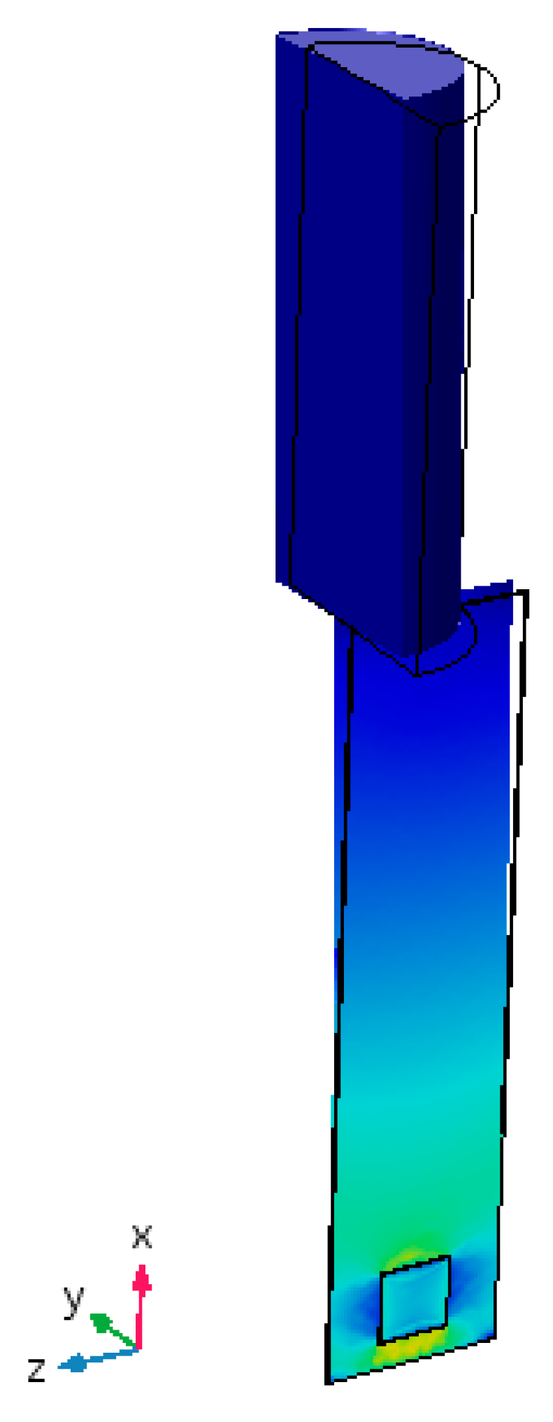
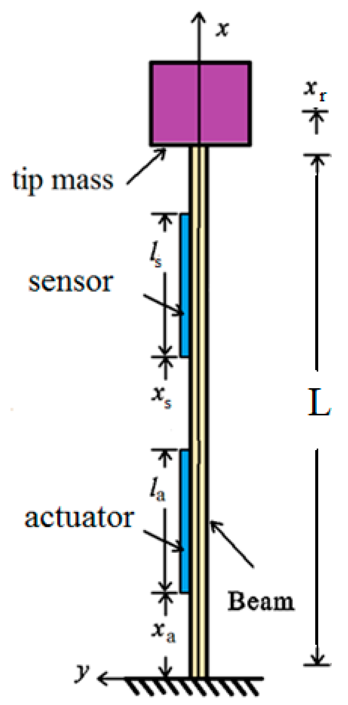
Figure 1 shows the schematic of the problem. The schematic of the aero-elastic system, as illustrated in Figure 1 and Figure 2, is an elastically-mounted D-shaped prism on a cantilever beam which is exposed to galloping fluctuations in the cross-flow direction. The slender beam (255 × 40 mm) has a D-shaped cylinder tip (70 × 60 mm) made of cardboard to capture the fluid flow energy. Here the D-shaped geometry is used for the experiment as it has maximum energy harvesting efficiency between simple shapes. However, with respect to the theory presented here, the other geometries could also be used with corresponding length, width, and aerodynamic coefficients in the presented formulas. Stability conditions for the PPF are obtained numerically and experimentally. With the intention to suppress and control such an aero-elastic coupled system, the system comprised of a sensor and actuator made of PZT is attached to the cantilever leg, as understood from Figure 2.

The kinetic energy of the aero-elastic coupled system is formed up from kinetic energy of the beam (with the mass per length of ${\overline{m}}_b$), kinetic energy of the piezoelectric sensor (with the mass per length of ${\overline{m}}_s$), kinetic energy of the piezoelectric actuator (with the mass per length of ${\overline{m}}_a$), and kinetic energy of the tip mass (with the mass per length of ${\overline{m}}_r$) as:

$$T=\frac{1}{2}{\displaystyle \underset{0}{\overset{L}{\int }}{\overline{m}}_b{\dot{u}}^{2}dx+}\frac{1}{2}{\displaystyle \underset{x_s}{\overset{x_s+h_s}{\int }}{\overline{m}}_s{\dot{u}}^{2}dx+}\frac{1}{2}{\displaystyle \underset{x_a}{\overset{x_a+h_a}{\int }}{\overline{m}}_a{\dot{u}}^{2}dx+}\frac{1}{2}{\displaystyle \underset{0}{\overset{L_r}{\int }}{\overline{m}}_r{(\dot{u}(L)+x_r\frac{d}{dx}\dot{u}(L))}^{2}d{x}_r}$$

(1)

where $\frac{d}{dx}\dot{u}(L)$is the angular velocity ($\dot{\theta }$) of the element of tip mass and the distance x_r is measured from the beginning of the tip mass. By the use of the method of separation of variables (u = Φ(ξ)q(t)), where Φ(ξ) are the matrix of shape functions and q(t) are the matrix of modal coefficients. By means of the length of the cantilever beam L as length scale, we introduce the following non-dimensional quantities:

$$\xi =\frac{x}{L},\lambda =\frac{L_r^{}}{L}$$

(2)

The kinetic energy of the system could be rewritten as:

$$\begin{array}{l}T=\frac{1}{2}{\overline{m}}_{b}L{\dot{q}}^T\left({\displaystyle \underset{0}{\overset{1}{\int }}{\Phi }^T\Phi d\xi }\right)\dot{q}+\\ \frac{1}{2}{\overline{m}}_{s}L{\dot{q}}^T\left({\displaystyle \underset{{\overline{x}}_s}{\overset{{\overline{x}}_s+{\overline{h}}_s}{\int }}{\Phi }^T\Phi d\xi }\right)\dot{q}+\\ \frac{1}{2}{\overline{m}}_{a}L{\dot{q}}^T\left({\displaystyle \underset{{\overline{x}}_a}{\overset{{\overline{x}}_a+{\overline{h}}_a}{\int }}{\Phi }^T\Phi d\xi }\right)\dot{q}+\\ \frac{1}{2}{\overline{m}}_r{L}_r{\dot{q}}^T\left({\Phi }^T(1)\Phi (1)\right)\dot{q}+\\ \frac{1}{2}\left(\frac{1}{3}{\overline{m}}_r{L}_r{}^3\right){\dot{q}}^T\left({{\Phi }^{\prime }}^T(1){\Phi }^{\prime }(1)\right)\dot{q}+\\ \frac{1}{2}\left({\overline{m}}_r{L}_r\right){\dot{q}}^T\left({\Phi }^T(1){\Phi }^{\prime }(1)+{{\Phi }^{\prime }}^T(1)\Phi (1)\right)\dot{q}\end{array}$$

(3)

which can be simplified to $T=\frac{1}{2}{\dot{q}}^T{M}_t\dot{q}$ by the aid of the following symbols:

$$\begin{array}{l}{M}_t=\left({\overline{m}}_{b}L\right)M_b+\left({\overline{m}}_s{h}_s\right)M_s+\left({\overline{m}}_a{h}_a\right)M_a+\left({\overline{m}}_r{L}_r\right)M_r+\left(\frac{{\overline{m}}_r{L}_r}{3}\right)I_r+\left(\frac{{\overline{m}}_r{L}_r}{2}\right)S_r\\ where\{\begin{array}{l}{M}_b={\displaystyle \underset{0}{\overset{1}{\int }}{\Phi }^T\Phi d\xi }\\ M_s={\displaystyle \underset{{\overline{x}}_s}{\overset{{\overline{x}}_s+{\overline{h}}_s}{\int }}{\Phi }^T\Phi d\xi }\\ M_a={\displaystyle \underset{{\overline{x}}_a}{\overset{{\overline{x}}_a+{\overline{h}}_a}{\int }}{\Phi }^T\Phi d\xi }\\ M_r={\Phi }^T(1)\Phi (1)\\ I_r={{\Phi }^{\prime }}^T(1){\Phi }^{\prime }(1)\\ S_r={\Phi }^T(1){\Phi }^{\prime }(1)+{{\Phi }^{\prime }}^T(1)\Phi (1)\end{array}\end{array}$$

(4)

Additionally, the potential energy of the system is formed from the potential energy of the beam (with a Young’s modulus of E and I = w_bt_b³/12), potential energy of the piezoelectric sensor (with a Young’s modulus of E_p), and potential energy of the piezoelectric actuator (with a Young’s modulus of E_p) as:

$$\begin{array}{l}V=\frac{1}{2}EI{\displaystyle \underset{0}{\overset{L}{\int }}{\left(\frac{{\partial }^{2}u}{\partial x^2}\right)}^{2}dx+}\frac{E_p{w}_p{t}_p}{2}{\displaystyle \underset{x_s}{\overset{x_s+h_s}{\int }}{\left(\frac{t_b}{2}\frac{{\partial }^{2}u}{\partial x^2}-\frac{d_{31}}{t_p}v\right)}^{2}dx+}\\ \frac{E_p{w}_p{t}_p}{2}{\displaystyle \underset{x_a}{\overset{x_a+h_a}{\int }}{\left(\frac{t_b}{2}\frac{{\partial }^{2}u}{\partial x^2}-\frac{d_{31}}{t_p}v\right)}^{2}dx}\end{array}$$

(5)

which can be simplified by $V=\frac{1}{2}{q}^T{K}_{t}q+\frac{1}{2}{v}^T{C}_{v}v-q^{T}Bv$ by the aid of the following symbols:

$$K_t=\left(\frac{EI}{L^3}\right)K_b+\left(\frac{E_s{w}_s{t}_s{t}_b{}^2}{4L^3}\right)K_s+\left(\frac{E_a{w}_a{t}_a{t}_b{}^2}{4L^3}\right)K_a$$

(6)

where:

$$\begin{array}{l}{K}_b={\displaystyle \underset{0}{\overset{1}{\int }}{{\Phi }^{″}}^T{\Phi }^{″}d\xi }\\ K_s={\displaystyle \underset{{\overline{x}}_s}{\overset{{\overline{x}}_s+{\overline{h}}_s}{\int }}{{\Phi }^{″}}^T{\Phi }^{″}d\xi }\\ K_a={\displaystyle \underset{{\overline{x}}_a}{\overset{{\overline{x}}_a+{\overline{h}}_a}{\int }}{{\Phi }^{″}}^T{\Phi }^{″}d\xi }\\ v=\left[\begin{array}{cc}{v}_s& v_a\end{array}\right]\\ B=\left[\begin{array}{cc}\frac{E_s{w}_s{t}_b{d}_{31}}{2L}\left({\Phi }^{\prime }({\overline{x}}_s+{\overline{h}}_s)-{\Phi }^{\prime }({\overline{x}}_s)\right)& \frac{E_a{w}_a{t}_b{d}_{31}}{2L}\left({\Phi }^{\prime }({\overline{x}}_a+{\overline{h}}_a)-{\Phi }^{\prime }({\overline{x}}_a)\right)\end{array}\right]\\ C_v=\left[\begin{array}{cc}\frac{E_s{w}_s{h}_s{d}_{31}{}^2}{2t_s}& 0\\ 0& \frac{E_a{w}_a{h}_a{d}_{31}{}^2}{2t_a}\end{array}\right]\end{array}$$

(7)

and charge amplitude is given by:

$$Q=C_s{V}_s=E_p{w}_p{d}_{31}{\displaystyle \underset{x_s}{\overset{x_s+h_s}{\int }}\frac{t_b}{2}\frac{{\partial }^{2}u}{\partial x^2}dx}=\frac{t_b{E}_p{w}_p{d}_{31}}{2}\left(\frac{\partial u(x_s+h_s)}{\partial x}-\frac{\partial u(x_s)}{\partial x}\right)$$

(8)

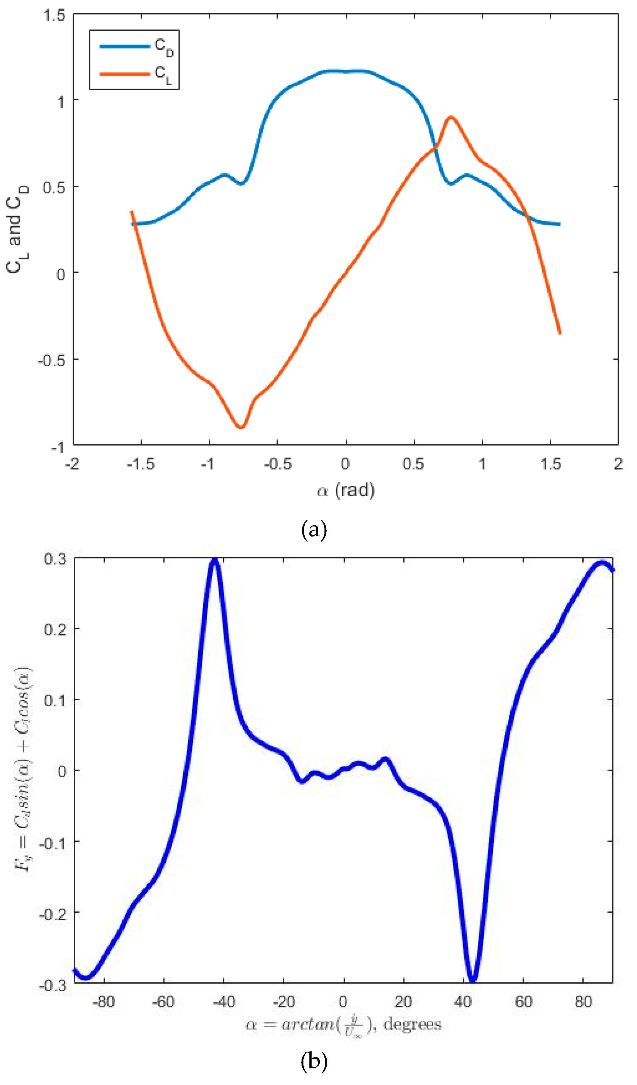
where $V_s=\frac{t_b{t}_s({\phi }^{\prime }(x_s+h_s)-{\phi }^{\prime }(x_s))}{2d_{31}}$. Figure 3 presents the lift and drag coefficient for D-shaped cross-section geometry and the effectiveness in normal direction. On the other hand the virtual work of the galloping force applied on the D-shaped could be found from:

$$\begin{array}{l}\delta W={\displaystyle \underset{0}{\overset{L_r}{\int }}}{F}_y\left(\delta u(L)+x_r\frac{d\delta u(L)}{d{x}_r}\right)d{x}_r\\ ={\displaystyle \underset{0}{\overset{L_r}{\int }}-}\left(F_{lift}\cos (\alpha )+F_{drag}\sin (\alpha )\right)\left(\delta u(L)+x_r\frac{d\delta u(L)}{d{x}_r}\right)d{x}_r\\ ={\displaystyle \underset{0}{\overset{L_r}{\int }}-}\left(\frac{1}{2}\rho U_{\infty }^{2}D\left(a_1\alpha -a_3{\alpha }^3\right)\right)\left(\delta u(L)+x_r\frac{d\delta u(L)}{d{x}_r}\right)d{x}_r\end{array}$$

(9)

where U_∞ is the free stream velocity, D is the diameter of the D-shaped tip mass and α is defined by:

$$\alpha =t{g}^{-1}\left(\frac{\dot{u}(L)+x_r\frac{d\dot{u}(L)}{d{x}_r}}{U_{\infty }}\right)\cong \frac{\Phi (L)+x_r{\Phi }^{\prime }(L)}{U_{\infty }}\dot{q}$$

(10)

Since the virtual work of the galloping force applied on the D-shaped could be rewritten in the form of:

$$\begin{array}{l}\delta W={\displaystyle \underset{0}{\overset{L_r}{\int }}-}\left(\frac{1}{2}\rho D\left(a_1{U}_{\infty }\left(\Phi (L)+x_r{\Phi }^{\prime }(L)\right)\dot{q}-\frac{a_3{\dot{q}}^3}{U_{\infty }}{\left(\Phi (L)+x_r{\Phi }^{\prime }(L)\right)}^3\right)\right)\delta q^T\left({\Phi }^T(L)+x_r{{\Phi }^{\prime }}^T(L)\right)d{x}_r\\ =-\delta q^T{C}_1\dot{q}+\delta q^{T}C\dot{q}\end{array}$$

(11)

where:

$$C_1=\frac{1}{2}\rho D{L}_r{a}_1{U}_{\infty }\left(\begin{array}{l}{\Phi }^T(L)\Phi (L)+{{\Phi }^{\prime }}^T(L){\Phi }^{\prime }(L)\frac{L_r{}^2}{3}+\\ \left({{\Phi }^{\prime }}^T(L)\Phi (L)+{\Phi }^T(L){\Phi }^{\prime }(L)\right)\frac{L_r}{2}\end{array}\right)$$

(12)

and:

$$C=\frac{\rho D{L}_r{a}_3}{2U_{\infty }}\left(\begin{array}{l}\left({\dot{u}}_L^2+\frac{L_r{}^2}{2}{\dot{\theta }}_L^2\right){\Phi }^T(L)\Phi (L)+\frac{L_r}{L}\left({\dot{u}}_L^2+\frac{3L_r{}^2}{4}{\dot{\theta }}_L^2\right){{\Phi }^{\prime }}^T(L)\Phi (L)\\ +\frac{L_r}{L}\left(\frac{3{\dot{u}}_L^2}{2}+\frac{L_r{}^2}{4}{\dot{\theta }}_L^2\right){\Phi }^T(L){\Phi }^{\prime }(L)+{\left(\frac{L_r}{L}\right)}^2\left({\dot{u}}_L^2+\frac{L_r{}^2}{5}{\dot{\theta }}_L^2\right){{\Phi }^{\prime }}^T(L){\Phi }^{\prime }(L)\end{array}\right)$$

(13)

where:

$${\dot{u}}_L^2={\dot{q}}^T{\Phi }^T(L)\Phi (L)\dot{q},L^2{\dot{\theta }}_L^2={\dot{q}}^T{{\Phi }^{\prime }}^T(L){\Phi }^{\prime }(L)\dot{q}$$

(14)

2.1. The Method of Multiple Scales for the Single-Mode

In this section, a perturbation analysis is achieved with the purpose of study the special effects of mass, stiffness, force coefficients, and damping of the single-mode model of the system on the frequency of the response, amplitude, and phase shift of galloping of the aero-elastic structure. The Poincaré-Linstedt method provides a way to construct asymptotic approximations of periodic solutions, but it cannot be used to obtain solutions that evolve periodically on a slow time-scale. The method of multiple scales (MMS) is a more general approach in which we introduce one or more new ‘slow’ time variables for each time scale of interest in the problem (see [23,24,25] for more detail of MMS). It does not require that the solution depends periodically on the ‘slow’ time variables. For the solution of the one degree of freedom equation:

$$m\frac{d^{2}y(t)}{d{t}^2}+c\frac{dy(t)}{dt}+ky(t)=\frac{1}{2}\rho U_{\infty }D{L}_r{a}_1\frac{dy(t)}{dt}+\frac{1}{2}\rho D{L}_r\frac{a_3}{U_{\infty }}{\left(\frac{dy(t)}{dt}\right)}^3$$

(15)

we introduce the ansatz of:

$$y=y_0(\overline{t},\tau )+\epsilon y_1(\overline{\mathrm{t}},\tau )$$

(16)

where $\omega =\sqrt{\frac{k}{m},}\tau =\epsilon \overline{\mathrm{t}},\overline{\mathrm{t}}=\omega \mathrm{t}$. Hence, the equation of motion (Equation (15)) can be expressed as:

$$\frac{{\partial }^{2}y}{\partial {\overline{t}}^2}+y=\epsilon \left(\frac{\partial y}{\partial \overline{t}}+\beta {\left(\frac{\partial y}{\partial \overline{t}}\right)}^3\right)$$

(17)

which leads to the solution of this system:

$$\begin{array}{l}\frac{{\partial }^2{y}_0}{\partial {\overline{t}}^2}+y_0=0\\ \frac{{\partial }^2{y}_1}{\partial {\overline{t}}^2}+y_1=\frac{\partial y_0}{\partial \overline{t}}+\beta {\left(\frac{\partial y_0}{\partial \overline{t}}\right)}^3-2\frac{{\partial }^2{y}_0}{\partial \overline{t}\partial \tau }\end{array}$$

(18)

where $\epsilon =\frac{0.5\rho U_{\infty }D{L}_r{a}_1-c}{m\omega },\beta =\frac{\rho kDL{a}_3}{m{U}_{\infty }\left(-2c+\rho U_{\infty }D{L}_r{a}_1\right)}$. The solution of the first equation:

$$y_0=A(\tau )\cos (\overline{t}+\phi (\tau ))$$

(19)

could be replaced in second equation in Equation (17) to obtain:

$$\frac{{\partial }^2{y}_1}{\partial {\overline{t}}^2}+y_1=\sin (\overline{t}+\phi )\left(-A+\beta \frac{3A^3}{4}+2A^{\prime }\right)+2A{\phi }^{\prime }\cos (\overline{t}+\phi )$$

(20)

The occurrence of secular terms can be prevented when the coefficient of sine and cosine terms on the right-hand side of Equation (20) is considered zero to obtain:

$$\begin{array}{l}\phi ={\phi }_0^{}\\ A=\frac{1}{\sqrt{\frac{3\beta }{4}(e^{-\tau }-1)+A_0^{-2}{e}^{-\tau }}}\end{array}$$

(21)

Since the transient solution of Equation (14) is:

$$y=\frac{1}{\sqrt{\frac{3\beta }{4}(e^{-\epsilon \omega t}-1)+A_0^{-2}{e}^{-\epsilon \omega t}}}\cos (\omega t+{\phi }_0)$$

(22)

2.2. The Assumed Mode Expansion for Two Modes

If the two term assumed modes expansion utilized in u = Φ(ξ)q(t) then:

$$u(\mathrm{x},\mathrm{t})=q_1(t){\phi }_1(x)+q_2(t){\phi }_2(x)$$

(23)

The solution of $\frac{{\mathrm{d}}^4}{\mathrm{d}{\mathrm{x}}^4}\mathrm{Y}(\mathrm{x})-{\mathrm{c}}^2\left\{\frac{\mathsf{\rho }}{\mathrm{EI}}\right\}\mathrm{Y}(\mathrm{x})=0$ is $\mathrm{Y}(\mathrm{x})={\mathrm{a}}_1\sin \mathrm{h}(\mathsf{\beta }\mathrm{x})+{\mathrm{a}}_2\cosh (\mathsf{\beta }\mathrm{x})+{\mathrm{a}}_3\sin (\mathsf{\beta }\mathrm{x})+{\mathrm{a}}_4\cos (\mathsf{\beta }\mathrm{x})$so, for a cantilever beam, the constant could be found and rewritten as:

$$\begin{array}{l}{\phi }_1(x)=\cosh ({\beta }_{1}x)-\cos ({\beta }_{1}x)+\\ \frac{\cosh ({\beta }_{1}L)+\cos ({\beta }_{1}L)}{\sin ({\beta }_{1}L)+\sinh ({\beta }_{1}L)}\left(\sin ({\beta }_{1}x)-\sinh ({\beta }_{1}x)\right)\\ {\phi }_2(x)=\cosh ({\beta }_{2}x)-\cos ({\beta }_{2}x)+\\ \frac{\cosh ({\beta }_{2}L)+\cos ({\beta }_{2}L)}{\sin ({\beta }_{2}L)+\sinh ({\beta }_{2}L)}\left(\sin ({\beta }_{2}x)-\sinh ({\beta }_{2}x)\right)\end{array}$$

(24)

where $\cosh ({\beta }_{1}L)\cos ({\beta }_{1}L)+1=0$. Using the extended Hamilton’s principle, the equations of motion for the galloping controlled by piezoelectric sensor and actuator can be obtained from the equation:

$${\displaystyle \underset{t_1}{\overset{t_2}{\int }}}\left(\delta T+\delta W\right)dt=0$$

(25)

where δT and δW are the virtual kinetic energy and the total virtual work, respectively. Inserting Equations (1), (5), (11) and (23) into Equation (25) and integrating by parts, we obtain:

$$\delta q^T\left(M_t\ddot{q}+K_{t}q+Bv-\left(C_1+C\right)\dot{q}\right)+\delta v^T\left(C_{v}v-B^{T}q\right)=0$$

(26)

Based on the fact that δq and δv are independent and arbitrary the terms in parentheses should be zero that result in the subsequent system of ordinary equations of motion:

$$\begin{array}{l}{M}_t\ddot{q}+K_{t}q=-Bv+\left(C_1+C\right)\dot{q}\\ C_{v}v=B^{T}q\end{array}$$

(27)

The above time-varying and non-linear equations is solved by the MATLAB ode45 function, and the results are shown in Section 3.

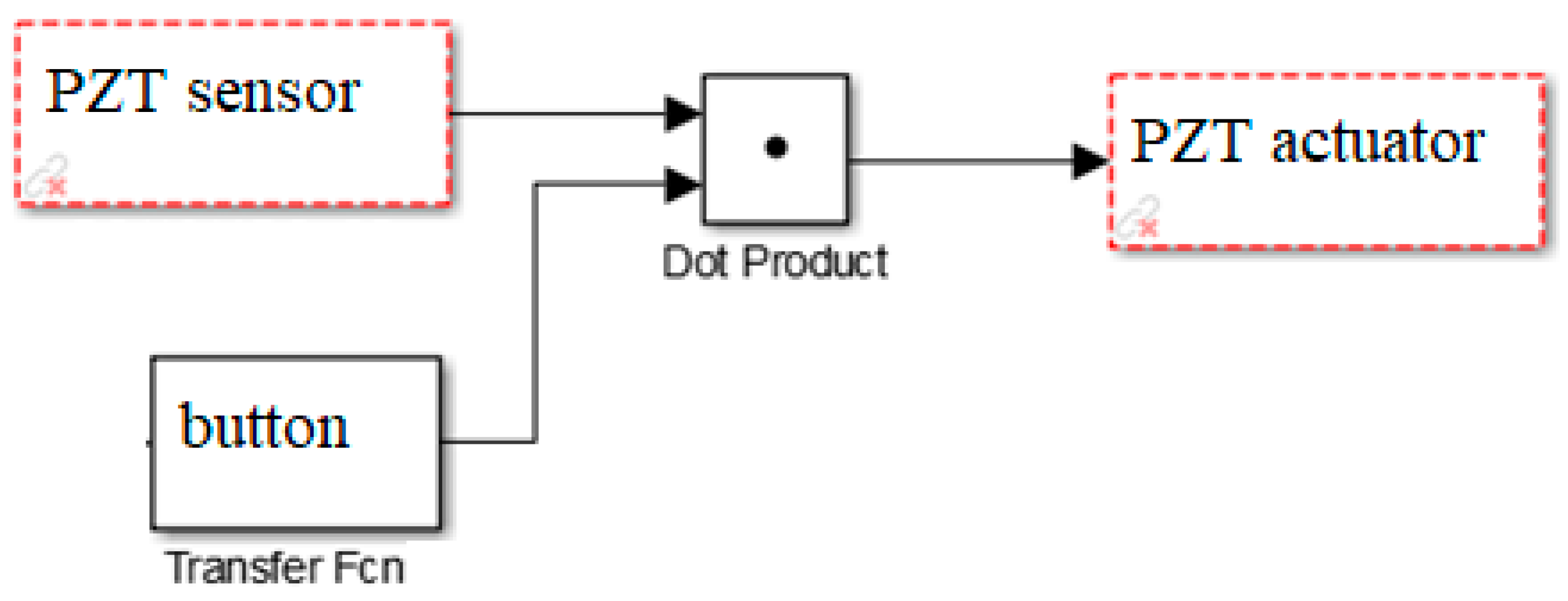
2.3. Positive Feedback Control of the Galloping Structures

To activate the vibration control of the beam, it is equipped with piezo-ceramic actuators and sensors. The positive position feedback (PPF) algorithm is assumed to control the single-input and single-output (SISO). For each mode a PPF is designed.

$$\begin{array}{l}{M}_t\ddot{q}+K_{t}q=-\frac{E_a{w}_a{t}_b{d}_{31}}{2L}\left({\Phi }^{\prime }({\overline{x}}_a+{\overline{h}}_a)-{\Phi }^{\prime }({\overline{x}}_a)\right)G_a{v}_a+\left(C_1+C\right)\dot{q}\\ v_s=G_s{\left(\frac{t_s{t}_b}{L{h}_s{d}_{31}}\left({\Phi }^{\prime }({\overline{x}}_s+{\overline{h}}_s)-{\Phi }^{\prime }({\overline{x}}_s)\right)\right)}^{T}q\\ {\ddot{Q}}_i+2{\zeta }_f{\omega }_i{\dot{Q}}_i+{\omega }_i^2{Q}_i=g_i{\omega }_i^2{q}_i\end{array}$$

(28)

where G_a and G_s have been added to represent the sensor and actuator amplifier gains, respectively.

We discuss how to design the single-input and single-output positive position feedback controller for a target structure by considering an Euler-Bernoulli beam. It is found that the theories developed in this study are capable of predicting the control system characteristics and its performance.

The closed-loop response of the beam to a wind excitation can be modeled by a nonlinear second-order differential equation, while the dynamics of the controller can be modeled by a linear second-order differential equation.The galloping structure studying here be made up of D-shaped cross-section with mass m and a cantilever which has the following governing equations:

$$\begin{array}{l}m\frac{d^{2}y(t)}{d{t}^2}+c\frac{dy(t)}{dt}+ky(t)=\frac{1}{2}\rho U_{\infty }D{L}_r{a}_1\frac{dy(t)}{dt}+\frac{1}{2}\rho D{L}_r\frac{a_3}{U_{\infty }}{\left(\frac{dy(t)}{dt}\right)}^3+\theta V_a(t)\\ \frac{d^2{V}_a(t)}{d{t}^2}+2{\xi }_F{\omega }_F\frac{d{V}_a(t)}{dt}+{\omega }_F{}^2{V}_a(t)=K_p{V}_s(t)\\ C_p\frac{d{V}_s(t)}{dt}+\frac{V_s(t)}{R}+\theta \frac{dy(t)}{dt}=0\end{array}$$

(29)

If the piezoelectric sensor be free of electrical load the equation of controlled system is:

$$\left(s^2+\left(2\xi \omega -\frac{1}{2m}\rho U_{\infty }D{L}_r{a}_1\right)s+{\omega }^2+\frac{{\theta }^2{K}_p}{m{C}_p\left(s^2+2{\xi }_F{\omega }_{F}s+{\omega }_F{}^2\right)}\right)Y=\frac{1}{2m}\rho D{L}_r\frac{a_3}{U_{\infty }}{\left(sY\right)}^3$$

(30)

The Routh-Hurwitz stability criterion with the coefficients of the characteristics polynomial of:

$$\begin{array}{l}{s}^4+\left(2{\xi }_F{\omega }_F+2\xi \omega -\frac{1}{2m}\rho U_{\infty }D{L}_r{a}_1\right)s^3+\left({\omega }_F{}^2+{\omega }^2\right)s^2+\\ \left(2{\xi }_F{\omega }_F{\omega }^2+2\xi \omega {\omega }_F{}^2-\frac{1}{2m}\rho U_{\infty }D{L}_r{a}_1{\omega }_F{}^2\right)s+\\ \left({\omega }_F{}^2{\omega }^2+\frac{{\theta }^2{K}_p}{m{C}_p}\right)=0\end{array}$$

(31)

leads to the following condition for the stability of linear part for the case of feedback frequency matches the natural frequency of the system:

$${\xi }_F>\frac{1}{4\omega m}\rho U_{\infty }D{L}_r{a}_1-\xi$$

(32)

and

$$K_p<\frac{m{C}_p{\omega }^4}{{\theta }^2}$$

(33)

As the for a fourth-order polynomial ($s^4+b_3{s}^3+b_2{s}^2+b_{1}s+b_0=0$), all the coefficients must be positive: $b_1<b_2{b}_3$ and$b_0{b}_3^2+b_1^2<b_1{b}_2{b}_3$.

3. Results

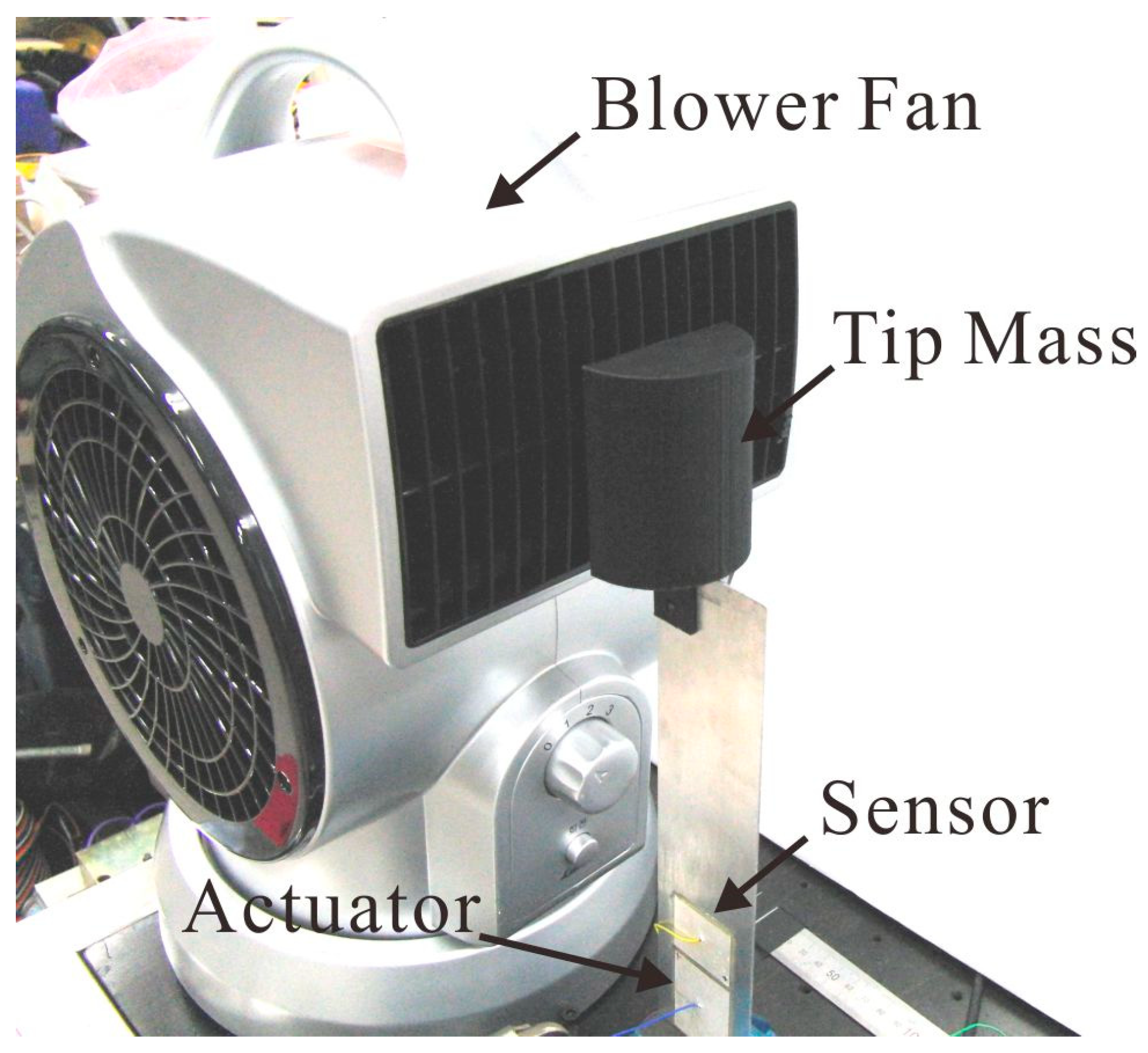
The experimental rig of a galloping elastic cantilever beam with a rigid mass (see Figure 1) was used to validate the theory by the parameters shown in

Table 1. Parameters of the simulation.

Parameter	Value	Parameter	Value	Parameter	Value	Parameter	Value
ζ	1.6815 × 10−4	bb, tb	40.1 mm	d31	−190 pm/V	xs	1 cm
ω	42.5 s−1	bp,a, tb,a	35.5 mm	Lb	29 cm	Ls	6 cm
ζF	0.3	bp,s, tb,s	15.5 mm	D,H	6.14 cm	xa	7.5 cm
fF	7.6 s−1	Ep	69 Gpa	m	78 g	La	1.5 cm

[17]. The piezo-ceramic wafer PZT-5A was bonded to the beam to harvest transverse vibrational mechanical energy in electric charge form. A blower fan is used for wind source while the signals are processed in MATLAB software (2018a, academic license, Dongguk univeristy, Seoul, Korea, 2018) via a SIMULINK interface. During the course of using PPF (with block diagram of Figure 4) to suppress the vibration of a beam excited by wind velocity, the parameters of the simulation model are given in Table 1. The experimental rig provided is shown in Figure 5. It consists of a blower fan, tip mass, cantilever beam, sensor, and actuator. 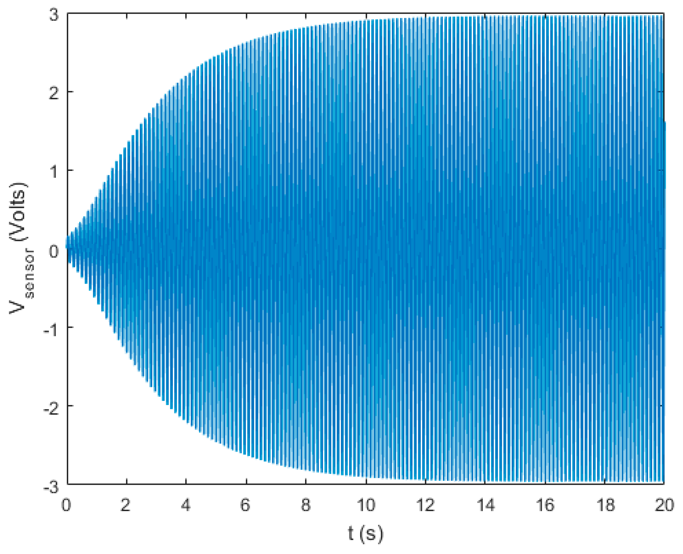The results presented in Figure 6 show the simulated sensor voltage for an initial velocity of 1 m/s starting from static equilibrium. As shown, the system reaches a steady state condition for less than 15 s.

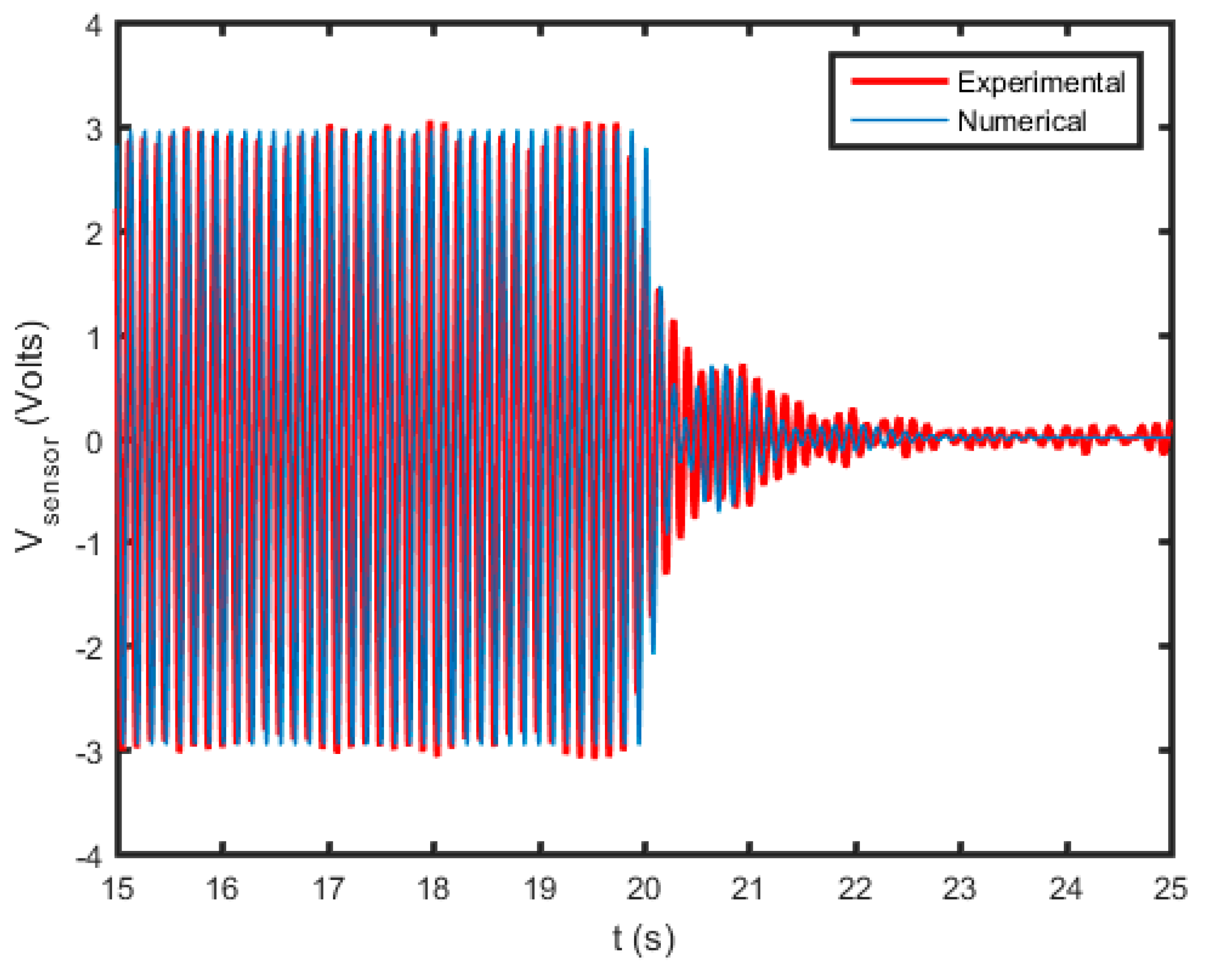
Figure 7 presents a comparison of numerical and experimental results of [17] for the sensor voltage where the FPP is applied at t = 20. As shown, the experimental results in Figure 7 are in 85% agreement with the model in Equation (2) for the estimated parameters of the system.

4. Conclusions

In this study, the control of a galloping-based energy harvester system, consisting of a D-shaped prism mounted on a cantilever beam by means of a positive position feedback (PPF) controller, is investigated. The system is simulated with the assumed mode method and represented by two coupled second-order ordinary differential equation systems. Then, the positive position feedback control by use of a sensor-actuator piezoelectric is implemented on the system to suppress the galloping oscillations. The results shows that the PPF controller is a powerful method to decrease the galloping amplitude of the D-shaped prism. The numerical results are in a good agreement with experimental results. Engineering applications of the proposed method are with respect to the vibration suppression of the galloping structure to the wind gustiness. The limitation of the proposed method is described in Equation (33).

References

1. Novak, M. Galloping oscillations of prismatic structures. J. Eng. Mech. 1972, 98, 27–46. [Google Scholar]
2. Dai, H.L.; Wang, L.; Qian, Q.; Ni, Q. Vortex-induced vibrations of pipes conveying fluid in the subcritical and supercritical regimes. J. Fluids Struct. 2013, 39, 322–334. [Google Scholar] [CrossRef]
3. Chang, W.K.; Pilipchuk, V.; Ibrahim, R.A. Fluid flow-induced non-linear vibration of suspended cables. Nonlinear Dyn. 1997, 14, 377–406. [Google Scholar] [CrossRef]
4. Blevins, R.D. Flow-Induced Vibrations; Van Nostrand Reinhold: New York, NY, USA, 1990. [Google Scholar]
5. Jun, L. Positive position feedback control for high-amplitude vibration of a flexible beam to a principal resonance excitation. Shock Vib. 2010, 17, 187–203. [Google Scholar] [CrossRef]
6. Abdelkefi, A.; Nuhait, A.O. Modeling and performance analysis of cambered wing-based piezoaeroelastic energy harvesters. Smart Mater. Struct. 2013, 22, 095029. [Google Scholar] [CrossRef]
7. Barrero-Gil, A.; Alongso, G.; Sanz-Andres, A. Energy harvesting from transverse galloping. J. Sound Vib. 2010, 329, 2873–2883. [Google Scholar] [CrossRef]
8. Paidoussis, M.P. Fluid–Structure Interactions: Slender Structures and Axial Flow; Academic Press: London, UK, 1998. [Google Scholar]
9. Baz, A.; Ro, J. Active control of flow-induced vibrations of a flexible cylinder using direct velocity feedback. J. Sound Vib. 1991, 146, 33–45. [Google Scholar] [CrossRef]
10. Mehmood, A.; Abdelkefi, A.; Akhtar, I.; Nayfeh, A.H.; Nuhait, A.; Hajj, M.R. Linear and nonlinear active feedback controls for vortex-induced vibrations of circular cylinders. J. Vib. Control 2012, 20, 1137–1147. [Google Scholar] [CrossRef]
11. Wang, L.; Liu, W.B.; Dai, H.L. Aeroelastic galloping response of square prisms: The role of time-delayed feedbacks. Int. J. Eng. Sci. 2014, 75, 79–84. [Google Scholar] [CrossRef]
12. Blevins, R.D. The effect of sound on vortex shedding from cylinders. J. Fluids Struct. 1985, 161, 217–237. [Google Scholar] [CrossRef]
13. Huang, X.Y. Feedback control of vortex shedding from a circular cylinder. Exp. Fluids 1996, 20, 218–224. [Google Scholar] [CrossRef]
14. Akhtar, I.; Nayfeh, A.H. Model based control of laminar wake using fluidic actuators. J. Comput. Nonlinear Dyn. 2010, 5, 041015. [Google Scholar] [CrossRef]
15. Gattulli, V.; Ghanem, R. Adaptive control of flow-induced oscillations including vortex effects. Int. J. Nonlinear Mech. 1999, 34, 853–868. [Google Scholar] [CrossRef]
16. Hasheminejad, S.M.; Rabiee, A.H.; Jarrahi, M.; Markazi, A.H.D. Active vortex-induced vibration control of a circular cylinder at low Reynolds numbers using an adaptive fuzzy sliding mode controller. J. Fluids Struct. 2014, 50, 49–65. [Google Scholar] [CrossRef]
17. Kim, G.-Y.; Kwak, M.K.; Shin, J.-H. Active Vibration Control of Galloping Structure. Available online: http://m.dbpia.co.kr/Journal/ArticleDetail/NODE07184982 (accessed on 7 December 2018).
18. Walshe, D.E.; Wootton, L.R. Preventing wind-induced oscillations of structures of circular section. Proc. Inst. Civil Eng. 1979, 47, 1–24. [Google Scholar] [CrossRef]
19. Quadrante, L.A.R.; Nishi, Y. Amplification/suppression of flow-induced motions of an elastically mounted circular cylinder by attaching tripping wires. J. Fluids Struct. 2014, 48, 93–102. [Google Scholar] [CrossRef]
20. Holmes, P.J. Center manifolds, normal forms and bifurcations of vector fields with application to coupling between periodic and steady motions. Phys. D 1981, 2, 449–481. [Google Scholar] [CrossRef]
21. Owen, J.C.; Bearman, P.W.; Szewczyk, A.A. Passive control of VIV with drag reduction. J. Fluids Struct. 2001, 15, 597–605. [Google Scholar] [CrossRef]
22. Savadkoohi, A.T.; Vaurigaud, B.; Lamarque, C.H.; Pernot, S. Targeted energy transfer with parallel non-linear energy sinks, part II: Theory and experiments. Nonlinear Dyn. 2012, 67, 37–46. [Google Scholar] [CrossRef]
23. Kevorkian, J.; Cole, J.D. Multiple Scale and Singular Perturbation Methods; Springer: Berlin, Germany, 1996; ISBN 0-387-94202-5. [Google Scholar]
24. Bender, C.M.; Orszag, S.A. Advanced Mathematical Methods for Scientists and Engineers; Springer: Berlin, Germany, 1999; pp. 544–568. ISBN 0-387-98931-5. [Google Scholar]
25. Nayfeh, A.H. Perturbation Methods; Wiley–VCH Verlag: Weinheim, Germany, 2004; ISBN 0-471-39917-5. [Google Scholar]
Figure 1. Schematic of the problem.
Acoustics 01 00005 g001
Figure 2. Front view of concentrated mass at the end of a cantilever beam.
Acoustics 01 00005 g002
Figure 3. Force coefficient for D-shaped cross-section geometry: (a) lift and drag, and (b) effectiveness in normal direction.
Acoustics 01 00005 g003
Figure 4. Applied voltage model for the FPP method.
Acoustics 01 00005 g004
Figure 5. Experimental setup [17].
Acoustics 01 00005 g005
Figure 6. Simulated sensor voltage for the initial velocity of 1 m/s started from static equilibrium.
Acoustics 01 00005 g006
Figure 7. Comparison of numerical and experimental [17] for sensor voltage where the FPP applied at t = 20.
Acoustics 01 00005 g007