Classic Evans’s Drop Corrosion Experiment Investigated in Terms of a Tertiary Current and Potential Distribution

Abstract

Background: Evans’s drop is a classic corrosion experiment that is nearly 100 years old, and it is analogous to other corrosion systems promoted by O₂ gradients. The availability of more robust finite element software packages opens the possibility to reach a deeper understanding of these kind of corrosion systems. Methodology: In order to solve the problem, the model includes the governing mass transport diffusion and migration equation and the material balance in a nonsteady state by the finite element method. This is performed using COMSOL Multiphysics to predict the tertiary current and potential distribution considering the geometry, reaction kinetics, and mass transport for each ionic species. Significant Findings: A simulation of the tertiary current and potential distribution of the Evans’s drop corrosion experiment on an iron surface is presented. An oxygen concentration difference of 0.18 mol m⁻³ between the center and the drop periphery sets up a potential difference of 60 mV which acts as a corrosion driving force. Reaction kinetics are described by Tafel equations. Results include the evolution of concentration profiles for OH⁻, Fe²⁺, Fe³⁺, Fe(OH)₂, and Fe(OH)₃.

1. Introduction

Within the group of experiments developed by U. R. Evans, the “drop experiment” remains one of the most remarkable, colorful, and classic experiments in corrosion, as reported by Professor U. R. Evans in 1925 [1,2]. This clever experiment is based on the use of a drop of aqueous saline solution (e.g., NaCl or KCl), placed on a clean, polished, iron surface. This simple experiment convincingly demonstrates that aqueous corrosion results of both oxidation and reduction electrochemical reactions. These take place simultaneously on the iron surface and render invalid the idea that the corrosion of iron is purely a chemical process, as was believed for a long period of time.

Although it has been almost 100 years since the Evans’s drop experiment was conceived, it remains within the scope of scientists. This is due to its similarity with other natural corrosion systems such as the water line corrosion and differential aeration cells [1,2,3]. In addition, the Evans’s drop experiment is also considered to be an illustrative experiment in classrooms and laboratories during introductory corrosion courses. There are studies in the literature concerning experimental measurements of the potential distribution developed across the surface of an Evans’s drop by using the Kelvin probe technique [4]. Furthermore, corrosion products on the metal surface formed during the oxidation and reduction reactions have been analyzed by means of in situ RAMAN spectroscopy. The formation of two zones with different types of oxides was found. These were detected depending on the type of material, medium and pH [5]. Other techniques applied to investigate this system complement and deepen the knowledge of the original experiment proposed by Professor Evans. A couple of examples are the kinetic studies of iron dissolution and potential changes in the presence or absence of oxygen [6,7,8]. Moreover, other experiments such as measuring in situ oxygen diffusion coefficients in water–air interfaces can also be relevant to the experiment [8]. The above-mentioned reports have been mostly devoted to describing the mechanisms involved during the corrosion process and the prevention of its effects. In that sense, the resolution of the mass transport governing equations that describe this system can add additional information, such as the effects of oxygen concentration differences and a strategy to validate models with experimental results. A work that involves time-dependent mathematical modelling of the under-deposit corrosion for an Evans’s drop model was presented by Chang et al. [2]. These authors solved the conservation equations for each one of the ionic species, local electroneutrality, homogeneous reactions, and the formation of precipitates with the purpose of modeling the Evans’s drop experiment without defining the anodic and cathodic regions a priori.

In general, electrochemical systems are usually investigated by taking into account different factors that determine the deepness of the analysis. A primary current distribution considers electrical parameters only. A secondary current distribution considers electrical and kinetic factors, and a tertiary current distribution involves electrical and kinetic parameters, as well as the mass transfer of electrochemical species.

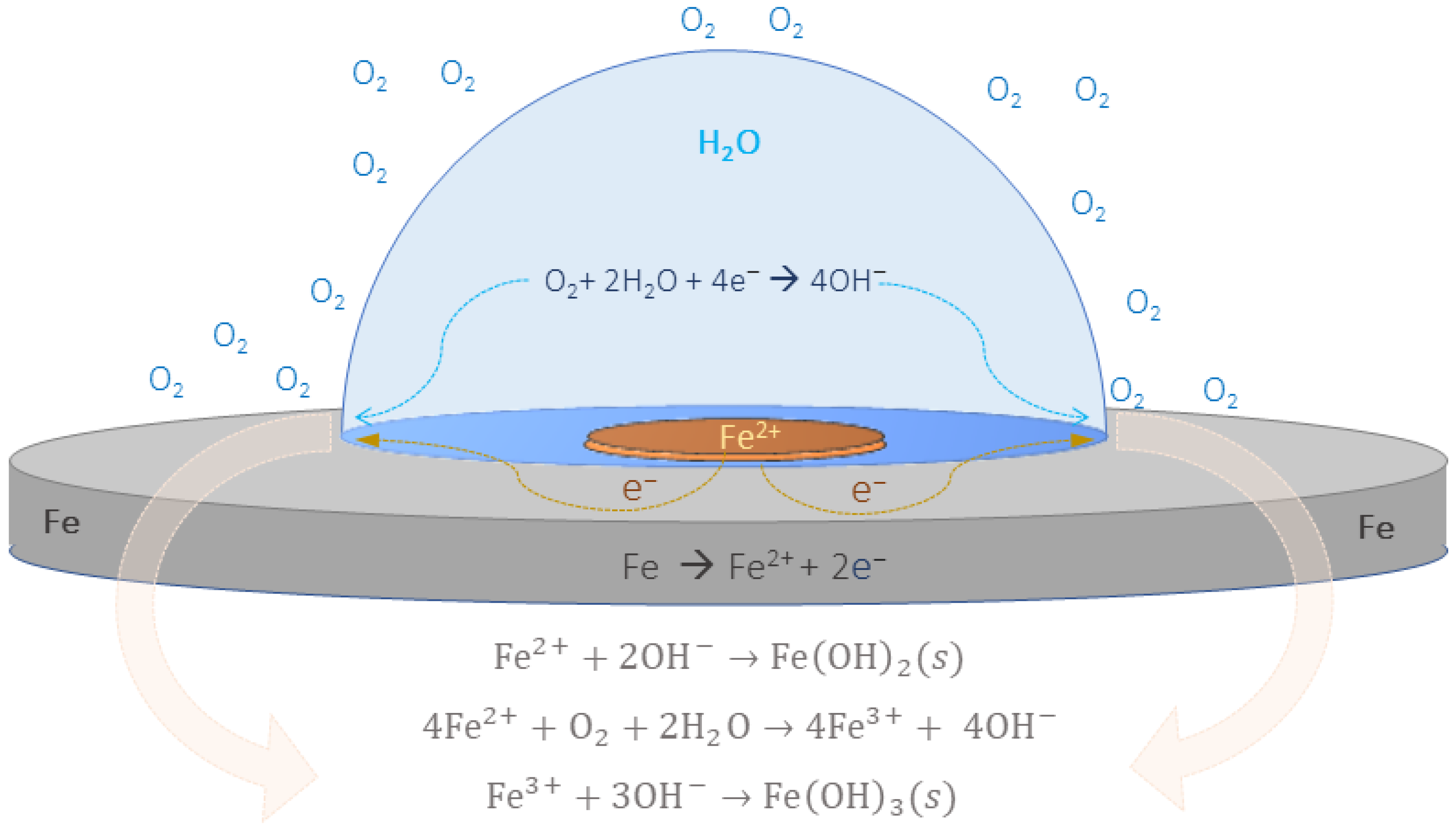
This work aims to simulate the tertiary current and potential distribution on iron covered by a saline drop. The model considers the oxidation of active Fe to form ferrous ions Fe²⁺, and the reduction of O₂ to form OH⁻, the mass transfer diffusion and migration of each ionic species, the reaction of Fe²⁺ with OH⁻ to produce Fe(OH)₂, and the reaction of Fe(OH)₂ with oxygen to produce Fe(OH)₃ as shown in Figure 1.

2. Materials and Methods

Evans’s drop experiments were performed on the surface of mild steel 1018 samples. Samples that were successively polished with abrasive paper grits (500 to 2000) to guarantee a smooth surface of known average surface roughness (R_A = 25 μm). The Evans’s solution was prepared by mixing 1 mL of potassium chloride 0.5 M, 1 mL of potassium ferricyanide 50 mM and 50 µL of 1% phenolphthalein in ethanol. A drop of solution (ca. 300 μL) was placed at the center of a recently abraded clean iron sheet using a micropipette. After a few minutes (ca. 15 min), color changes became evident at the center and periphery of the drop. Calculations were performed using COMSOL Multiphysics 5.1 software, on a PC with an i7 processor, 16GB RAM, 256 SSD. An extrafine free triangular geometry mesh was used for the finite element calculations. Five additional contour layers were added to the top and the bottom of the hemispherical cap to improve accuracy. Total simulation time was set to 600 seconds, with a 5 seconds time step.

3. Theory

The set of reactions considered in the model appears listed below. The equilibrium potentials are calculated in terms of concentrations and the Nernst’s equation.

$$\mathrm{Fe}\rightleftarrows {\mathrm{Fe}}^{2+}+2{\mathrm{e}}^{-}$$

(1)

$${\mathrm{O}}_2+2{\mathrm{H}}_2\mathrm{O}+4{\mathrm{e}}^{-}\rightleftarrows 4{\mathrm{OH}}^{-}$$

(2)

$$4{\mathrm{Fe}}^{2+}+{\mathrm{O}}_2+2{\mathrm{H}}_2\mathrm{O}\rightleftarrows 4{\mathrm{Fe}}^{3+}+4{\mathrm{OH}}^{-}$$

(3)

$${\mathrm{Fe}}^{2+}+2{\mathrm{OH}}^{-}\rightleftarrows \mathrm{Fe}{\left(\mathrm{OH}\right)}_2$$

(4)

$$2\mathrm{Fe}{\left(\mathrm{OH}\right)}_2+\frac{1}{2}{\mathrm{O}}_2+{\mathrm{H}}_2\mathrm{O}\rightleftarrows 2\mathrm{Fe}{\left(\mathrm{OH}\right)}_3\mathrm{or}{\mathrm{Fe}}_2{\mathrm{O}}_3\ast 3{\mathrm{H}}_2\mathrm{O}$$

(5)

It is assumed that the flux of all species in solution is described by the Nernst–Planck’s equation. This equation includes the diffusion, migration, and convection terms Equation (6), respectively:

$${\mathit{N}}_{\mathit{i}}=-D_i\nabla c_i-z_{i}F{u}_i\nabla \varnothing +\mathit{v}{c}_i$$

(6)

where D_i, is the diffusion coefficient of the species i, c_i is the concentration, z_i is the electrical charge of species i, F is Faraday’s constant, u_i is the ionic mobility, $\varnothing$ is the potential and v is the velocity vector. In our model, it is assumed to be a stagnant solution, therefore the convection term is absent.

The nonsteady state material balance for the system in terms of the divergence of the flux is described by Equation (7):

$$\frac{\partial C_i}{\partial t}=-\nabla ·{\mathit{N}}_{\mathit{i}}+R_i$$

(7)

where R_i is the production term of species i, and t is the time. The total current density, i, in terms of the flux is given by Equation (8):

$$i=-F{\displaystyle \sum }{z}_i{\mathit{N}}_{\mathit{i}}$$

(8)

The electrode surface allows to set up the boundary condition for the electrolyte potential, where i_loc,m (SI units: A/m²) are the local individual electrode reaction current densities and n denotes the unit vector normal to the electrode surface. The i_loc depends on the kinetic expression and the overpotential, which is defined in terms of the equilibrium potential at the anode and cathode Equations (14) and (15).

The total current density, $i$, is given by the sum of the local cathodic currents:

$$\mathit{n}·i={\displaystyle \sum _m{i}_{loc,m}}$$

(9)

Although for a primary current and potential distribution the potential at the electrode surface is considered constant assuming a fast kinetics, for a secondary and tertiary current and potential distribution it depends on the reaction kinetics at the solid surface. The potential at each electrode is equal to the difference between the potential at the solid and solution Equation (10).

$$E_{electrode}={\varphi }_s-{\varphi }_l$$

(10)

$E_{cell}$ is defined as the potential difference between the solid phases of the two electrodes Equation (11) and assuming the potential at cathode, ${\varphi }_{s,c}=0$, as a reference, we obtain Equation (12).

$$E_{cell}={\varphi }_{s,a}-{\varphi }_{s,c}={\varphi }_{s,a}$$

(11)

$$E_{cell}={\varphi }_{s,a}$$

(12)

In terms of the overpotential, Equation (12) turns into Equation (13).

$$\eta =E_{electrode}-E_{eq}$$

(13)

Thus, the anodic and cathodic overpotentials are represented by Equations (14) and (15), respectively.

$${\eta }_a=E_{electrode}-E_{eq,a}$$

(14)

$${\eta }_c=E_{electrode}-E_{eq,c}$$

(15)

On the other hand, the oxidation reaction kinetics of Fe and the reduction reaction kinetics of O₂ are described by Tafel’s equations, which are adjusted to the local current density of the metal according to Equations (16) and (17), where $b_a$ and $b_c$ are the Tafel slopes, and $i_{o,a}$ is the exchange current density, for the Fe oxidation, and $i_{o,c}$ is the exchange current density for the O₂ reduction.

$$i_{loc,a}=i_{0,a}{e}^{\frac{2.3{\eta }_a}{b_a}}$$

(16)

$$i_{loc,c}=-i_{0,c}{e}^{-\frac{2.3{\eta }_c}{b_c}}$$

(17)

The current density for the oxygen reduction reaction (ORR) is coupled to the O₂ flux as a boundary condition, the flux being proportional to the current density according to Faraday’s laws of electrolysis:

$$\mathit{n}·\mathit{N}=\frac{\nu i_{loc,c}}{nF}$$

(18)

where F is Faraday’s constant (96,485 C mol⁻¹), $\nu$ is the stoichiometric coefficient for the ORR, and n is the number of electrons involved in the reaction. In this model, the following two initial and boundary conditions are considered:

The typical mol fraction of oxygen in dry air at room temperature is equal to 0.2095, which corresponds to 0.2 mol m⁻³. It is assumed as the oxygen concentration at the solution/air interface.

$$C_{ref}=0.2\mathrm{mol}{\mathrm{m}}^{-3}$$

(19)

The initial concentration of O₂ inside the drop is assumed to be 0.02 mol m⁻³.

The electrode kinetics for the ORR is described by the following expression:

$$i_{loc,c}=-\left(\frac{c}{C_{ref}}\right)i_{0,c}{10}^{-\frac{{\eta }_c}{b_c}}$$

(20)

The flux vector for isolated boundaries is zero.

$$\mathit{n}·\mathit{N}=0$$

(21)

The set of differential equations with the initial and boundary conditions is solved in a nonstationary steady state, assuming an integration time of 600 s. Usually, it takes a similar time for equilibrium to be achieved and this is a typical time needed to carry out a practical experiment. The parameters used in the simulation are summarized in

Table 1. Parameters and constants used for the simulation.

Symbol	Value [9]	Description
r	0.005 m	Drop radius
T	298 K	Temperature
K	2.5 S m−1	Electrolyte conductivity
R	8.3144 J K−1 mol−1	Universal gas constant
pO2	21278 Pa	Partial oxygen pressure
O2 concentration	0.2 mol m−3	Oxygen concentration on the drop’s surface
bc for ORR on Fe	0.12 V	Cathodic Tafel slope [9]
ba for Fe = Fe2+	0.04 V	Anodic Tafel slope [9]
io,c for ORR on Fe	4 × 10−9 A m−2	Exchange current density for ORR on Fe [9]
io,a for Fe = Fe2+	0.01 A m−2	Exchange current density for Fe = Fe2+ [9]
D_O2	1.96 × 10−9 m2 s−1	Oxygen diffusion coefficient [9]
D_OH−	5.26 × 10−9 m2 s−1	Hydroxide diffusion coefficient [10]
D_H2O	2.30 × 10−9 m2 s−1	Water diffusion coefficient
D_Fe3+	0.61 × 10−9 m2 s−1	Diffusion coefficient of Fe3+ in solution [10]
D_Fe2+	0.72 × 10−9 m2 s−1	Diffusion coefficient of Fe2+ in solution [10]
D_Cl−	2.032 × 10−9 m2 s−1	Diffusion coefficient of Cl− in solution [10]
D_K+	1.957 × 10−9 m2 s−1	Diffusion coefficient of K+ in solution [10]

For the calculation of the current and potential distribution in the Evans’s drop, oxygen gradients, current, and fluxes of all species are considered in the solution.

.

4. Results and Discussion

A time sequence of images illustrating the evolution of the Evans’s drop experiment on the surface of a freshly polished iron plate is shown in Figure 2. Once the droplet of saline solution with the indicators added is dropped on the iron surface, it immediately starts developing a blue color at the central anodic part due to the oxidation of Fe to produce ferrous ions, Fe²⁺, which react with ferricyanide ions in solution, Fe(CN)₆³⁻, to form an insoluble precipitate of Prussian blue, Fe₄[Fe(CN₆)]₃. Released electrons during the Fe oxidation move to the periphery of the drop, where O₂ is reduced at the cathodic areas producing hydroxyl ions, OH⁻, while the Fe surface remains bright [3]. In the process, the pH of the periphery increases, and the phenolphthalein changes the color of the solution from colorless to magenta as it is evidenced in the images. On the other hand, ferrous ions that do not react with ferricyanide at the center diffuse and migrate in solution, reacting with hydroxyl ions coming from the drop´s periphery to produce either ferrous hydroxide or react with incoming O₂ to produce ferric ions. The former ones react with hydroxyl ions in solution to produce ferric hydroxide [9]. The complete set of reactions taken into consideration in the system for the calculations were summarized previously in Equations (1)–(5).

While maintaining standard temperature and pressure conditions, it takes about 15 min for this experiment to be completed. It becomes evident from Figure 2, that the geometry of the drop plays a key role in setting up an O₂ gradient concentration and establishing anodic and cathodic zones (i.e., differential aeration cells). The oxygen is consumed by the cathodic, oxygen reduction, reaction. Replenishment of this oxygen from the air is more rapid at the periphery of the drop, where the liquid layer is thinner than at the center. Therefore, the cathodic reaction predominates in the periphery of the drop. Even if any anodic spots develop in this area, the high hydroxyl ions concentration will precipitate the Fe²⁺ ions as fast as they pass into solution, thus sealing these anodic areas. On the other hand, at the drop´s center the lack of O₂ builds up an anodic zone where Fe oxidizes to Fe²⁺.

The oxygen concentration gradient sets up a potential difference that promotes the oxidation and reduction reactions. This potential difference can be estimated by knowing the oxygen and hydroxyl ion concentrations at different locations. A simple calculation of the potential difference between the drop’s center and the periphery, based on the oxygen reduction reaction (Equation (2)), and Nernst’s Equation (22) can be performed. For instance, if we consider an oxygen concentration of 0.2 mol m⁻³ and the calculated hydroxyl ion concentration of 0.5 mol m⁻³ at the periphery along with an assumed O₂ concentration of 0.02 mol m⁻³ and a calculated 0.05 mol m⁻³ hydroxyl ion concentration at the drop’s center, a potential difference of 43 mV is obtained.

$$E=0.401V+\frac{0.059}{4}log\left[\frac{O_2}{{\left[O{H}^{-}\right]}^4}\right]$$

(22)

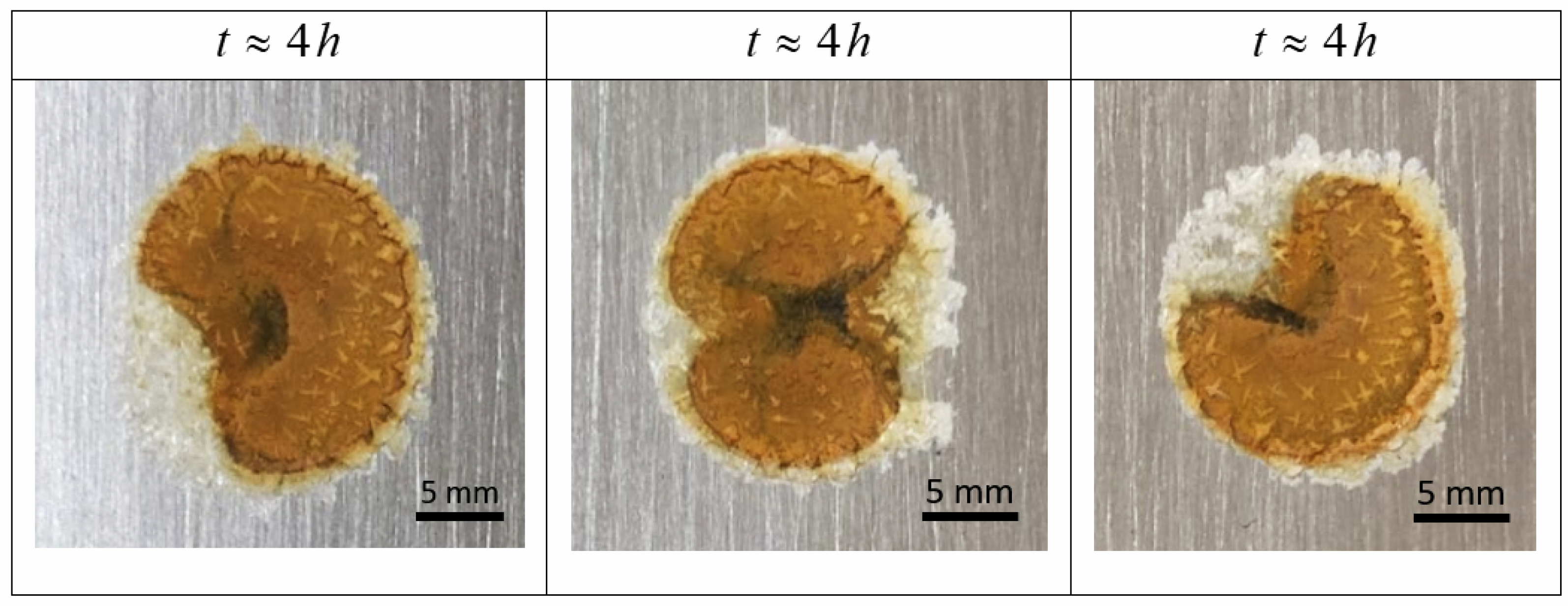
By allowing the saline drop to dry for about 4 h, the potassium chloride crystals precipitate mostly in the periphery and a ferric oxy-hydroxide stain appears in the whole area [5]. The shape of the rust stain depends on either how the solution was dropped on the iron surface or how it was distributed. Figure 3 shows the appearance of the rust stain in three different experiments. For all of them the KCl concentration was reduced to 0.25 M and the ferricyanide and phenolphthalein indicators were avoided to prevent color interference. At the central area some pits in the iron metal are also evidenced.

As abovementioned, a relevant parameter in Evans’s drop experiment is the potential difference set up along the radius caused by O₂ concentration gradients. In that sense, the corrosion process can be controlled by O₂ mass transfer through the drop, thus the mathematical simulations could allow us to visualize how the O₂ concentration gradient evolves. It requires to use a tertiary current and potential distribution to make a better modelling of the system. One set of potential difference calculations between the anodic and cathodic regions as a function of time is presented in Figure 4. The potential difference between the drop’s center to the periphery after 600 s, (i.e., the time it takes the experiment to be performed) is ca. 30 mV, while initially it was predicted to be 60 mV. These calculated potentials are similar to the ones measured experimentally with the Kelvin probe technique reported by Chen et al. [4]. At the center of the drop, there is a less noble potential of 92 mV, which increases at the cathodic region of the periphery, reaching ca. 103 mV after 5 s. A simulated potential distribution for an Evans´s drop model along the electrode surface shows a maximum 100 mV potential difference between the center and the periphery of the droplet for a surface covered with precipitates [2].

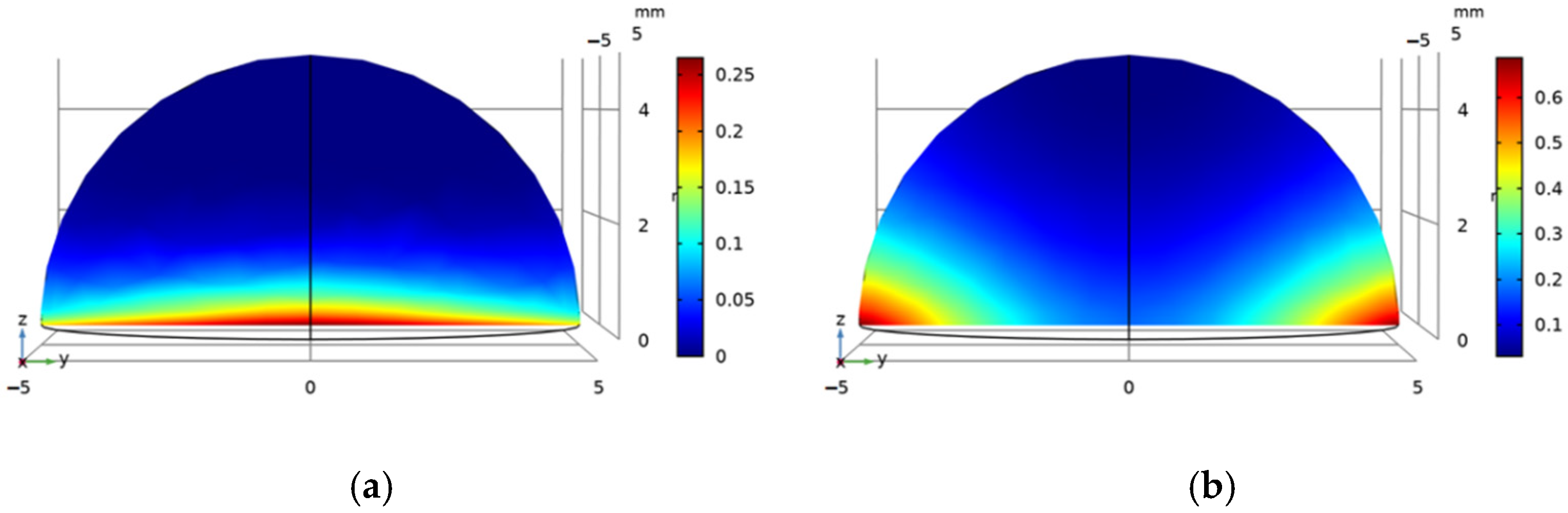
A simulation of the current and potential distribution for the whole system is shown in Figure 5a, where the arrows emerging from the central zone (anodic region) move toward the periphery (cathodic region). A similar result has been reported for an analogous experiment modeled with Butler–Volmer’s equation on a Zn surface reported by Venkatraman [11]. They also predicted the movement of charged ions in a solution promoted by diffusion and migration caused by the electric field. In both systems, the results approximate the ones calculated for a primary current distribution, without taking into consideration kinetics and mass transfer [12,13]. Accordingly, the equipotential lines are parallel to the electrode surface and perpendicular to the current lines. On the other hand, Figure 5b shows the oxygen concentration profile that develops through the electrolyte. The O₂ concentration value at the solution/air interface is the highest, approaching 0.2 mol m⁻³, which indeed is the boundary condition value used in the simulation, while at the center of the drop, the calculated O₂ concentration approaches 0.02 mol m⁻³.

Since the water column height at the center of the drop is thicker than at the edges, ca. 5 mm, it offers more resistance to oxygen diffusion than at the periphery. Thus, it takes a longer time for O₂ to diffuse and reach the Fe surface. This behavior agrees with the results observed in Figure 5b, where the red colors mean a higher O₂ concentration. This effect is more evident in Figure 6, where the simulation of the concentration profiles is presented. There, a comparison of the oxygen concentration at two different positions over a period of 600 s is shown. As shown, Figure 6a represents the variation of the oxygen concentration on the horizontal axis (0 < r < 5). Likewise, Figure 6b shows the oxygen concentration profile from the center of the drop moving perpendicular to the metal surface to the solution/air interface (r = 0, 0 < h < 5). It is clearly observed how the concentration of O₂ decreases near the periphery, where the oxygen is consumed by the cathodic reaction.

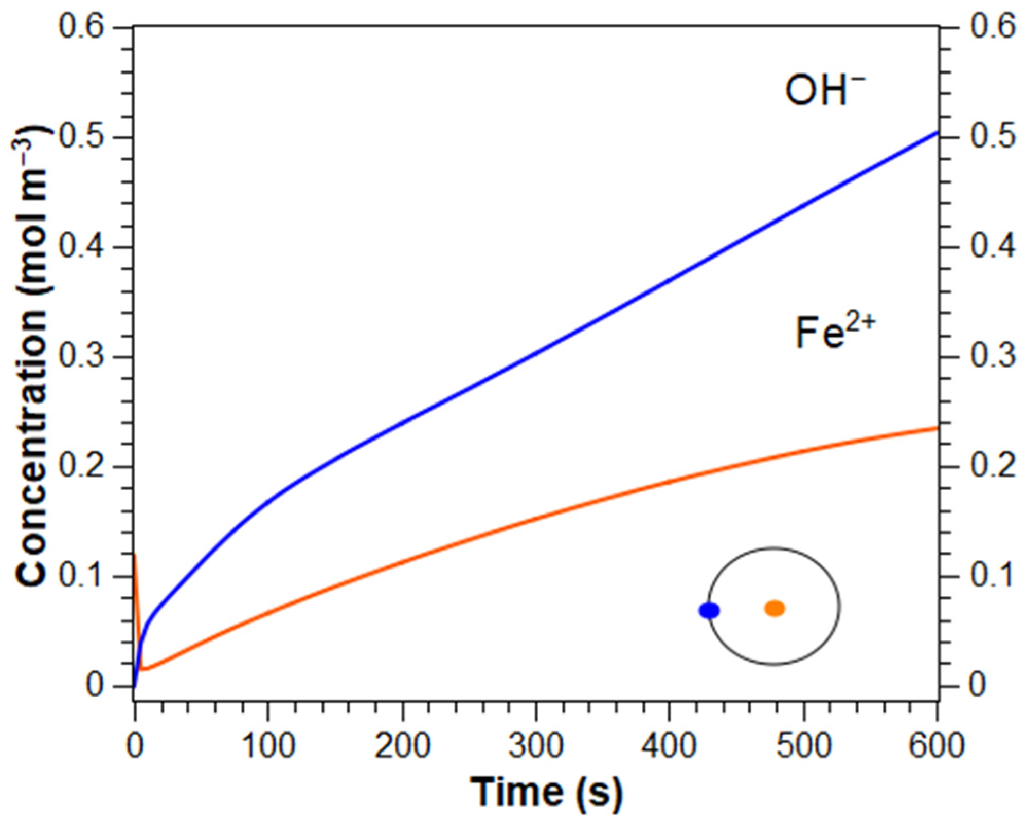
On the other hand, the oxidation of Fe takes place mainly at the center of the drop. Therefore, there is a rapid buildup in the concentration of ferrous ions Fe²⁺ that diffuse and migrate into the solution toward the periphery of the drop, owing to both the concentration and electric field gradients in Figure 7a. The maximum concentration of hydroxyl ions calculated in the periphery is 0.5 mol m⁻³, equivalent to an alkaline pH of 10.69 (Figure 7b), while at the center it may reach a pH 6.00 under the anode deposits [3]. Chang et al. reported a much slighter alkaline conditions at the periphery with a pH equal to 7.12. These authors suggest that the Fe(OH)₃ is mainly formed at this condition. However, it is more likely for the pH to be more alkaline since phenolphthalein turns into magenta color at pH 10, as it is observed in the Evan’s drop experiment.

The iron oxidation reaction at the drop’s center supplies the electrons for the oxygen reduction reaction at the periphery for the formation of OH⁻ ions (Figure 8). Oxidation and reduction kinetics on the iron surface are commonly described by Tafel expressions, however, we have also taken into account that the corrosion rate for this system is also limited by O₂ mass transfer [9,13].

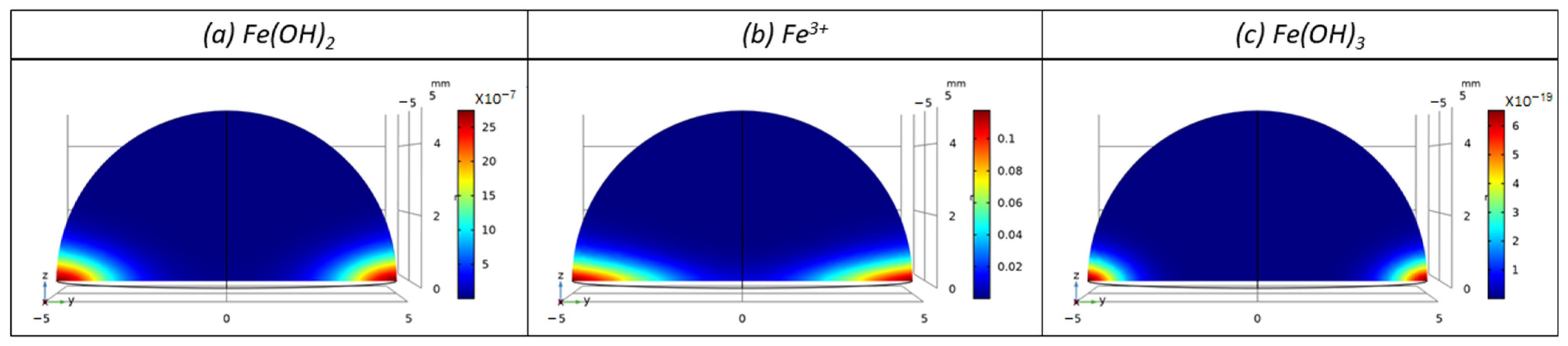
The complete group of species produced in the Evans’s drop is summarized in Figure 9. Figure 9a shows the concentration profile of Fe(OH)₂. Since the highest OH^- concentration is at the periphery and Fe²⁺ can travel by diffusion and migration, the highest concentration of Fe(OH)₂ appears near to the drop edges [14]. When the Fe²⁺ ions come in contact with the dissolved oxygen at the periphery, they oxidize to ferric ions, Fe³⁺. In a similar process, ferric ions, Fe³⁺, react with hydroxyl ions in solution and form ferric hydroxide, or as a result of the oxidation of Fe(OH)₂ in the presence of O₂ as shown in Figure 9b. The formation of ferric ions takes place to a lesser degree, due to the scarcity of Fe³⁺ in solution as it is observed in Figure 9c.

Figure 10 shows the concentration profiles of all the species considered in the Evans’s drop calculations, namely Fe²⁺, Fe³⁺, OH⁻, O₂, Fe(OH)₂, and Fe(OH)₃ through the base radius at the electrode surface for a time of 600 s. Once the experiment is completed, it can be observed that the concentration of hydroxyl ion OH⁻ is ca. 0.06 mol m⁻³ which is equivalent to a pH of 9.77 at the center of the drop. This pH value tends to increase towards the periphery, reaching a value of 0.5 mol m⁻³, equivalent to a pH of 10.69. The increment in the pH values is associated with a constant flux of oxygen coming from the surrounding air as well as the fact that the oxidation is maintained. The concentration of O₂ was considered constant at the solution/air interface (0.2 mol m⁻³).

Similar simulations can be performed to investigate other systems where there are oxygen concentration gradients, such as a corrosion line and oxygen concentration cells [15]. The performed simulation allowed us to predict the conditions required to promote corrosion and help to clearly determine where species are formed.

5. Conclusions

This work presented a simulation of the tertiary current distribution during the classical Evans’s drop experiment, which allowed the graphic visualization of the evolution of concentration profiles of species involved in iron corrosion as a function of time. The oxygen concentrations difference (0.18 mol m⁻³) between the center and periphery of the drop established a potential difference of 60 mV that agreed with experimental results published in the literature with a Kelvin probe technique. However, this potential difference evolved with time reaching a value of 30 mV at the end of the experiment according with the simulations. The O₂ consumption and replenishing zones were located at the edges of the drop and its profiles determined as a function of the position. An increase in the pH from the initial value of 6 at the center of the drop to a value of 10.69 after 600 s at the drop edges was calculated. The evolution profiles of Fe²⁺ and Fe³⁺ and the formation of Fe(OH)₂ were also predicted. Fe(OH)₂ formed in solutions took place at the edges due to the Fe²⁺ diffusion in the electrolyte and its reaction with the produced hydroxyl ions. The formation of Fe(OH)₃ (1 × 10⁻¹⁹ mol m⁻³) occurred mostly at the drop’s periphery where the oxygen concentration was higher. This study helped to achieve a better understanding of a classical corrosion experiment by considering the main iron oxidation and reduction reactions; however, it can be improved by including the formation of other oxides and the experimental evaluation of the oxygen concentration and pH across the droplet.