Minimum Noise Fraction Analysis of TGO/NOMAD LNO Channel High-Resolution Nadir Spectra of Mars

Abstract

NOMAD is a suite of spectrometers on the board of the ESA-Roscosmos Trace Gas Orbiter (TGO) spacecraft and is capable of investigating the Martian environment at very high spectral resolution in the ultraviolet–visible and infrared spectral ranges by means of three separate channels: UVIS (0.2–0.65 μm), LNO (2.2–3.8 μm), and SO (2.3–4.3 μm). Among all channels, LNO is the only one operating at infrared wavelengths in nadir-viewing geometry, providing information on the whole atmospheric column and on the surface. Unfortunately, the LNO data are characterized by an overall low level of signal-to-noise ratio (SNR), limiting their contribution to the scientific objectives of the TGO mission. In this study, we assess the possibility of enhancing LNO nadir data SNR by applying the Minimum Noise Fraction (MNF), a well-known algorithm based on the Principal Components technique that has the advantage of providing transform eigenvalues ordered with increasing noise. We set up a benchmark process on an ensemble of synthetic spectra in order to optimize the algorithm specifically for LNO datasets. We verify that this optimization is limited by the presence of spectral artifacts introduced by the MNF itself, and the maximum achievable SNR is dependent on the scientific purpose of the analysis. MNF application study cases are provided to LNO data subsets in the ranges 2.627–2.648 μm and 2.335–2.353 μm (spectral orders 168 and 189, respectively) covering absorption features of gaseous H₂O and CO and CO₂ ice, achieving a substantial enhancement in the quality of the observations, whose SNR increases up to a factor of 10. While such an enhancement is still not enough to enable the investigation of spectral features of faint trace gases (in any case featured in orders whose spectral calibration is not fully reliable, hence preventing the application of the MNF), interesting perspectives for improving retrieval of both atmospheric and surface features from LNO nadir data are implied.

1. Introduction

The ExoMars Trace Gas Orbiter (TGO) spacecraft launched in 2016 towards Mars as a joint ESA-Roscosmos mission and is still currently operating. Its main scientific objectives are to search for and investigate several trace gases in the Martian atmosphere [1], with a particular focus on methane, thanks to a set of spectrometers at very high spectral resolution. Following the heritage of previously flown high-resolution spectrometers, like SOIR-SPICAV on the Venus Express spacecraft [2] and PFS [3] and SPICAM [4] on the Mars Express mission, the TGO spacecraft carries two spectrometers: the Atmospheric Chemistry Suite (ACS, [5]) and the Nadir and Occultation for Mars Discovery (NOMAD, [6,7]). Both instruments can take advantage of solar occultation observations to achieve a signal-to-noise ratio (SNR) high enough for detecting the narrow and shallow spectral lines diagnostic of trace gases and isotopologues. In particular, the NOMAD instrument consists of three channels operating in different spectral ranges and with different observing modes (Section 2). In the present study, we focus on the data registered by the NOMAD-LNO (Limb, Nadir, and Occultation) infrared channel in nadir-viewing geometry, which is characterized by an overall low SNR level (Section 2.1) and would therefore benefit from noise-reduction procedures. A well-known technique that is commonly adopted to improve SNR within spectroscopic data is the Principal Component (PC) transform. The PC algorithm diagonalizes the spectral covariance matrix of a statistically meaningful ensemble of data and transforms it into a new space of eigenvectors ordered with decreasing variance. This diagonalization enables us to discriminate between the transform components of the signal due to the source, characterized by correlated variations, and those due to the noise, randomly fluctuating without correlation (see [8] for a comprehensive review). However, this approach does not provide a definite trend for how the noise increases with the number of components adopted in the transformation [9].

The Minimum Noise Fraction (MNF) transform is a PC-based technique that, instead, provides transformation components (eigenvectors) ordered with the content of increasing random, uncorrelated noise [9,10,11]. This estimation relies on the comparison between the data and a sample of purely random noise that must be provided to the algorithm as well. The MNF is usually applied to hyperspectral imaging datasets to improve performance in spectral classifications of surface minerals or for other geological applications (e.g., [11,12,13,14,15]).

Here, we apply the transform to high-spectral-resolution data of the Martian surface and atmosphere acquired by the LNO channel in nadir-viewing. Our goal is to assess the improvement of SNR achievable by applying the MNF technique to these observations, establishing both the gain and the limitations of the approach. In Section 2, we provide some details on the instrument characteristics and operations necessary to understand the rationale behind the analysis. Section 3 deals with MNF’s theoretical background and tuning of its parameters, while the test on LNO observations is presented in Section 4. Results are discussed in Section 5, while Section 6 is dedicated to the conclusions.

2. The NOMAD Instrument

NOMAD spectrometers each have their own optical bench but share the same interface with the satellite. Two channels operate in the infrared (LNO and SO, covering the spectral ranges 2.2–3.8 μm and 2.3–4.3 μm, respectively) and one in the ultraviolet–visible spectral range (UVIS, covering the 0.2–0.65 μm range). UVIS operates in nadir-viewing, limb-viewing, and solar occultation geometries, whereas the SO channel is dedicated to solar occultation measurements, directly observing the Sun’s extinction through the atmosphere during every sunset and sunrise for each TGO polar orbit. The Limb, Nadir, and Occultation channel (LNO) can work in all three observing modes, with most of the measurements dedicated to the nadir geometry, that is, looking at the sunlight reflected from the surface and atmosphere of Mars at an emission angle close to 0°. Nadir acquisitions are limited to latitudes between −75° and 75° in order to avoid dealing with too large solar incidence angles.

Among the three NOMAD spectrometers, LNO is the only one operating at infrared wavelengths in nadir-viewing geometry. With respect to the Solar Occultation channel (SO), whose sounding altitude is limited by the increased atmospheric extinction at low heights, LNO is conceived to provide information on the whole atmospheric column and, hence, also on species that could be only present close to the surface (e.g., CH₄ [16]). Potentially, it can also be used to investigate surface features, even if the instrumental characteristics (i.e., high spectral resolution, low spatial resolution, and limited instantaneous spectral range) are not optimized for such a purpose.

The design of both infrared channels is inherited from the Venus Express/Solar Occultation in the InfraRed (SOIR) spectrometer and consists of an échelle grating combined with a passband Acousto-Optical Tunable Filter (AOTF, see Section 2.1). This configuration enables a very high spectral resolution, about 0.15 cm⁻¹ and ~0.3 cm⁻¹ for SO and LNO, respectively.

While in-depth technical descriptions of NOMAD channels can be found in [6,7,17,18], in Section 2.1 and Section 2.2, we provide basic information about LNO channel data calibration and noise in order to give context to the presented analysis.

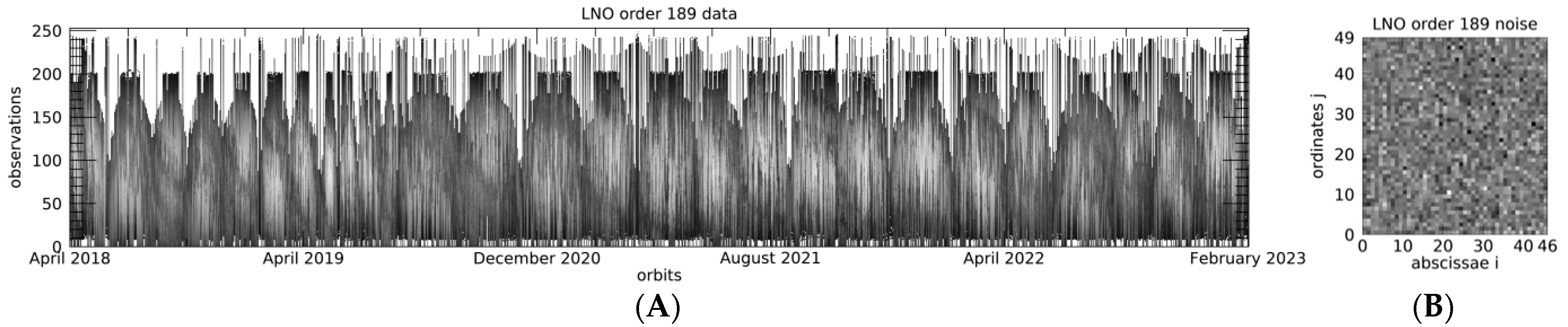
2.1. LNO Instrumental Characteristics and Noise

The LNO channel’s main instrumental characteristics related to the nadir observing mode are given in

Table 1. Instrumental characteristics of the NOMAD LNO channel for nadir observing geometry [6,7,19].

LNO Channel Instrumental Characteristics (NADIR)
Wavelength range λ	2.3–3.8 (μm)
Wavenumber range k	2630–4250 (cm−1)
Resolving power λ/Δλ	104
Field of view (FOV)	4 × 150 (arcmin2)
Instantaneous footprint (400 km orbit)	0.5 × 17.5 (km2)
Integration time per order	$\frac{15}{\mathrm{n}\mathrm{u}\mathrm{m}\mathrm{b}\mathrm{e}\mathrm{r} \mathrm{o}\mathrm{f} \mathrm{s}\mathrm{i}\mathrm{m}\mathrm{u}\mathrm{l}\mathrm{t}\mathrm{a}\mathrm{n}\mathrm{e}\mathrm{o}\mathrm{u}\mathrm{s}\mathrm{l}\mathrm{y} \mathrm{a}\mathrm{c}\mathrm{q}\mathrm{u}\mathrm{i}\mathrm{r}\mathrm{e}\mathrm{d} \mathrm{o}\mathrm{r}\mathrm{d}\mathrm{e}\mathrm{r}\mathrm{s}} (\mathrm{s})$
Detector	HgCdTe, 320 × 256 pixel
Signal-to-noise ratio (SNR)	20 (average)–80 (maximum)

.

The size of the slit of the LNO spectrometer provides a compromise between maximizing the signal entering the instrument and limiting the footprint size. With a 4 × 150 arcmin² slit, LNO reaches a spectral resolution of 0.3 cm⁻¹ at 3000 cm⁻¹ (resolving power λ/Δλ∼10,000) and an instantaneous footprint of 0.5 × 17.5 km². The actual footprint is significantly enlarged by motion smearing during the integration time and through spatial binning if performed on the acquisitions. The detector is a mercury–cadmium–telluride (HgCdTe) focal plane array (FPA), made up of 320 pixels along the spectral axis and 256 rows in the spatial direction.

Although the LNO detector is overall sensitive to the full 2.3–3.8 μm (2630–4250 cm⁻¹) spectral interval, the actual spectral range of an individual observation is defined by the AOTF transmission curve, which has a main central lobe about 22 cm⁻¹ wide, with the central wavelength selected through an internal radiofrequency generator. The AOTF’s response spectral width is matched to the width of one single order of diffraction of the échelle grating, and, for this reason, from now on, we will refer to each spectral window as “order”. Given this configuration, the data are not acquired simultaneously in the whole spectral range, and each order is characterized by a different spatial and temporal coverage.

Initially conceived to be actively cooled down to −100 °C, the instrument actually operates at about 0 °C due to a descoping that forced the removal of the cryo-radiator [6]. As a result, the instrument’s thermal background is the dominant SNR-limiting factor since it both increases the shot noise and prevents the use of long exposures, which could saturate the detector. As a noise mitigation strategy, on-board frame co-adding is used instead, adopting integration times shorter than 200 ms for each frame [18], even if detector readout impacts the number of acquisitions that can be made in a single measurement. For nadir observations, the resulting integration time for a LNO spectrum is obtained by dividing the duration of an observation cycle (15 s on average) by the number of diffraction orders contextually measured (6 at maximum). Such a configuration is able to yield SNR average values of about 20, taking into account the whole LNO spectral range. This moderate SNR value is the main factor preventing a wider exploitation of NOMAD infrared data in exploring the Martian surface and low-altitude atmosphere at a very high spectral resolution, and it is the reason for which we attempt to apply a noise reduction technique to the dataset (Section 3).

2.2. LNO Data Calibration

The in-depth calibration process for LNO data can be found in [20]. In short, raw data are radiometrically calibrated in radiance by taking into account optic transmission and detector sensitivity and incorporating the effects of the instrument’s temperature. On the other hand, no assumptions are made about the transmission curves of the AOTF and of the échelle grating (i.e., the Blaze function), whose peaks and shapes change from one order to the next and are not easily determined. As a result, the spectral shape of a LNO radiance spectrum is modulated by the shapes of these functions. The Blaze function is well approximated by a sinc function, while the AOTF transmission curve is better described by a combination of a sinc function with a Gaussian [19] and is characterized by the presence of secondary peaks (side-lobes) in addition to the main one. These side-lobes allow photons with wavelengths not pertaining to the selected order range to fall on the detector. This yields a partial mixing of the spectral information that cannot be removed by the calibration procedure and is more relevant at the edges of any order’s nominal spectral range. Conversion to reflectance is performed by using the direct Sun’s observations, occasionally acquired through the LNO occultation mode with very short integration times. The radiance is then converted to reflectance factor $R_F$ by dividing it by the solar flux at Mars and by the cosine of the solar incidence angle:

$$R_F(\lambda )=f_{SN}\frac{\pi L\left(\lambda \right)}{{\varphi }_{Sun}\left(\lambda \right)d_{Mars}^2}\times \frac{1}{{\mu }_0}$$

where $L\left(\lambda \right)$ is the nadir spectral radiance (W cm⁻² sr⁻¹ cm), ${\varphi }_{Sun}\left(\lambda \right)$ is the spectral solar flux at 1 astronomical unit (AU), $d_{Mars}$ is the Sun–Mars distance in AU, ${\mu }_0=\cos \left(\mathsf{\theta }\right)$ with θ being the solar incidence angle, and $f_{SN}$ a conversion factor taking into account the slightly different optical path between Sun and nadir observation modes. In principle, apart from a small residual coming from additive contributions from side-lobes, the instrumental modulations affecting the signal should cancel out in reflectance spectra, being present in both the Mars and the Sun observations. However, even if this turns out to be often the case in the central part of the orders’ range, where a nearly flat spectral reflectance continuum is found, it is not true in general. In fact, the AOTF- and blaze-induced modulations are found to significantly change among observations; hence, they also propagate to the reflectance factor conversion in the form of low-frequency oscillations of the spectral continuum, making the direct comparison of these data with radiative transfer simulations not trivial. In this study, we do not attempt to remove these modulations with any continuum fitting processing since this could potentially alter the low-frequency spectral signatures related to surface or aerosol features (see Section 4.3.1). Also, the spectral calibration has been found to slightly change among observations due to the thermal-induced mechanical stress of the detector. In this regard, reliable wavenumber calibration can only be obtained by fitting the positions of well-known solar lines, giving slightly different results for each observation [19].

3. Method Description and Synthetic Data Analysis

In this section, we describe the method behind our analysis. Section 3.1 provides a brief description of the MNF transform, while a test application of the technique to a synthetic dataset is provided in Section 3.2 and its subsections.

3.1. The Minimum Noise Fraction Transformation

In this study, we use the generalized MNF algorithm described in [9,11], consisting of two separate PC rotations. In-depth descriptions of the MNF transform are given in several dedicated papers (e.g., [21,22]) so we report only some basic information here.

Let us represent the LNO reflectance factor dataset as a two-dimensional array X consisting of a statistically significant number of observations, each having 320 spectral bands b. In the presence of a random noise N, the measured signal X can be written as:

X = S + N

(1)

where S represents the signal from the target. Under the assumption that the two components are uncorrelated, the covariance matrix of the dataset, ∑_X, is:

∑_X = ∑_S + ∑_N

(2)

where ∑_S and ∑_N are the covariance matrices of S and N, respectively. It is now possible to introduce the so-called noise whitening matrix W, which orthonormalizes ∑_N and contains the eigenvectors of ∑_N∑_X⁻¹:

W^T∑_N W = I

(3)

W∑_N ∑_X⁻¹ = EW

(4)

where E is a diagonal matrix of eigenvalues. By linearly transforming the initial dataset X with the noise whitening matrix W, we can obtain a new dataset Y in which the 320 bands are uncorrelated:

Y = W^TX

(5)

Let us now define the noise fraction, F, as the ratio of the variance of the noise, ν_N, to that of the total signal, ν_X, for each spectral band b:

F(b) = ν_N (b)/ν_X (b)

(6)

The eigenvalues in E, which by convention can be ordered as monotonically increasing, give the noise fraction of Y. Conversely, they provide the quantity (SNR + 1)⁻¹, giving information on the signal-to-noise ratio, ordered as decreasing. By keeping only the first N_e eigenvalues and inverting the transformation back to the initial data space, we can therefore obtain a dataset Z with enhanced SNR:

Z = (W⁻¹)^TI*Y

(7)

where I* is an identity matrix in which all diagonal elements, except for the first N_e ones, have been zeroed. It is worth noting that those pieces of information that are only present in a limited number of initial spectra could correspond to eigenvalues with values close to 1, hence providing SNR~0 [11]. Nevertheless, this issue can be overcome by applying the algorithm to data subsets in which the information content is more homogeneously distributed among observations (provided that the data statistics are still enough to ensure the computation of the ∑_X and ∑_N matrices; see Section 5.2). For our applications, we take advantage of the implementation of the MNF transform algorithm included in the ENVI^® software package, version 5.7 (Exelis Visual Information Solutions, Boulder, CO, USA, https://www.nv5geospatialsoftware.com/Products/ENVI, accessed on 7 December 2023).

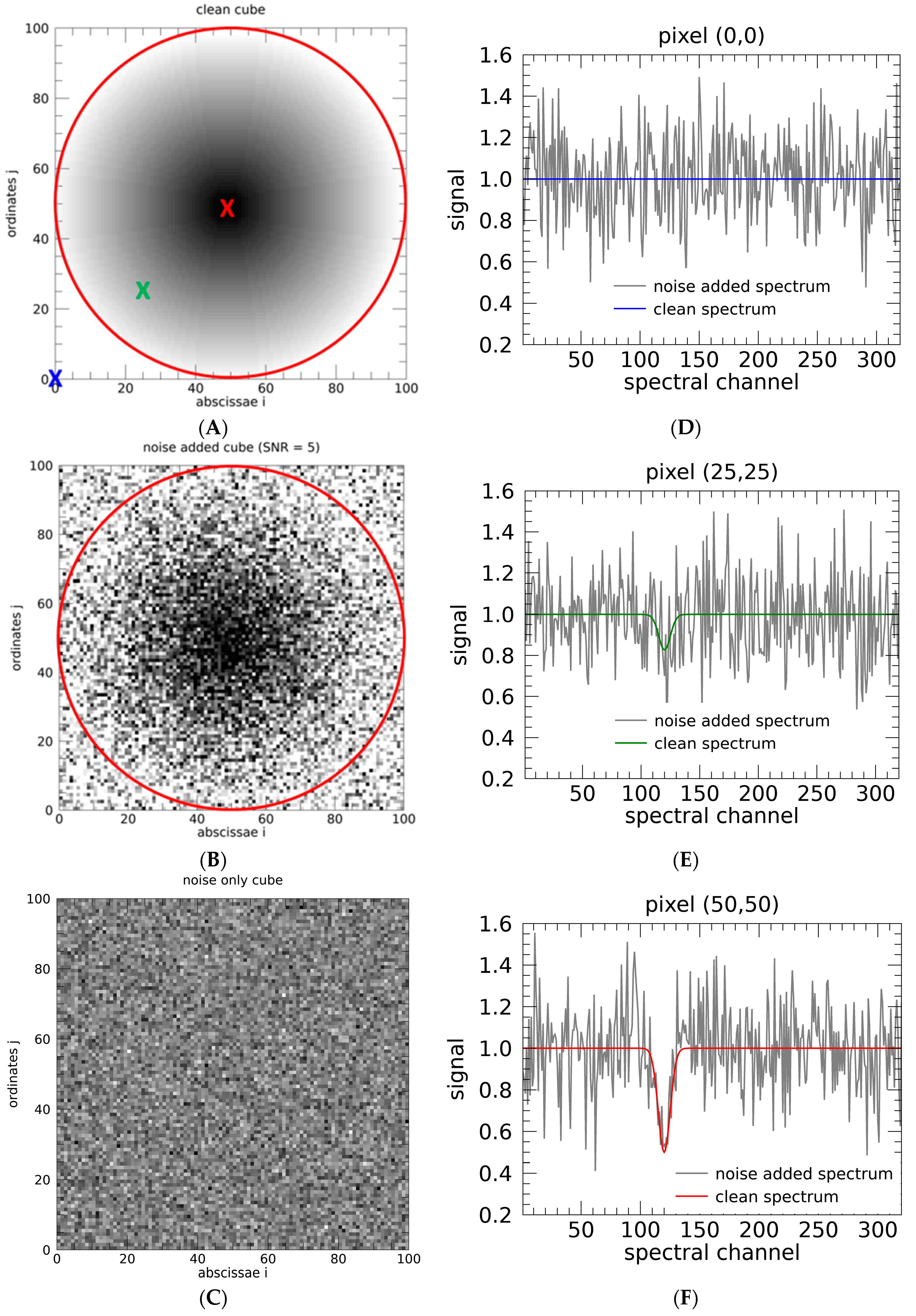
3.2. Synthetic Dataset Test

In order to test the MNF performances on LNO spectral data, we first apply it to a fully supervised, LNO-like synthetic dataset. Our purpose is to track the information content throughout the processing and, in particular, to study the optimal number of eigenvalues needed to be retained to meaningfully reconstruct the spectra (Section 3.2.1). The test also allows for verifying the spatial coherence between the reconstructed data and the original ones (Section 3.2.2).

We build three-dimensional synthetic datasets (cubes) with two spatial dimensions (100 by 100 pixels) and a third spectral one with 320 spectral channels (consistent with the number of bands of LNO; Section 2.1). The first cube contains correlated data in the form of an absorption band of variable intensity (Figure 1A), to which random Gaussian noise is added in order to simulate SNR values as low as 5 (Figure 1B). Such values set up the basis for reproducing some of the most critical noise conditions in LNO nadir data. The added noise is stored in a second cube (Figure 1C) and used for the noise covariance matrix computation. In the data cube, a Gaussian-shaped absorption band (denoted as band β from now on) is spectrally centered on channel 120 (the choice is arbitrary) and spatially located only inside a circular region with a radius of 50 pixels (Figure 1A). The band depth is set to decrease radially from the center (where it is 0.5, Figure 1F) to the boundaries of the circle, while its width is kept constant. Outside that, the band is not present at all, so this can be used as a zero control region (see Figure 1D,E).

We apply the MNF to the cubes shown in Figure 1B,C, respectively, to compute the covariance matrices ∑_X and ∑_N required by the algorithm. In output, we obtain 320 eigenvalues, which are ordered with an increasing noise fraction (Section 3.1). By back-transforming the data and retaining an increasing number of eigenvalues, it is possible to investigate how the information content is processed. If only a few eigenvalues are used (Figure 2B), very small fluctuations arise in the reconstructed spectra, yielding a very high SNR gain. However, it is worth noting that some spurious spectral features appear (shaped as both absorption and emission lines) in the zero control region, probably due to a selection effect acting on random fluctuations induced by the β band itself (Figure 2C). The presence of these artifacts represents a warning about information processing since they can potentially bias the distribution of spectral features in the transformed dataset. On the other hand, increasing the number of retained eigenvalues yields larger and larger fluctuations in the transformed spectra, making the artifacts less statistically meaningful but decreasing the SNR gain. We can therefore take advantage of such a phenomenon to estimate the number N_e of eigenvalues that need to be adopted for a statistically viable determination of the output noise.

3.2.1. Best SNR Gain

In order to estimate the statistical significance of the artifacts with respect to the number of MNF eigenvalues, for every spectrum in the zero control region, we compare the equivalent width values of β (derived by evaluating the spectral integrals of the band and of the continuum across the absorption) with those of the fluctuation amplitude of the spectral continuum (denoted as γ and evaluated far from the β band location). These two quantities are normally distributed with mean and standard deviation values (µ and σ, respectively) that depend on the number N_e of eigenvalues. As shown in Figure 3, due to the presence of the artifacts in the MNF-reconstructed data, we have systematically:

|μ_β ± σ_β| > |μ_γ ± σ_γ|

(8)

with |μ_γ ± σ_γ| that approaches |μ_β ± σ_β| as N_e increases. In Section 3.2.2, we will see how we can equate these two quantities in a conservative way; here, we report a more relaxed approach aimed at maximizing the SNR gain. Taking into account separately the + and – signs in (8), we derive the numbers N_e+ and N_e− for which the two sides of the equation become comparable within their errors (Figure 3), obtained by propagating the uncertainties of the normal distributions’ Gaussian fits. Then, the final number N_e for the data reconstruction is set as the maximum between N_e+ and N_e−. In our example, N_e+ = 3, N_e− = 4, and, hence, N_e = 4, yielded a SNR gain of 12 (output SNR = 60). This gain implies that, while in the non-processed cube (SNR = 5) β is already comparable to the noise when it is still 25% of its maximum equivalent width, the MNF processing can decrease this value down to 3%, in fact lowering the detection limit of β.

Such a criterion ensures the largest SNR gain while making the artifacts statistically not significant. It also provides the basis for practically characterizing the output noise in the reconstructed spectra. However, it is worth stressing that this method removes the spectral artifacts only statistically and is not totally reliable with individual observations, thus preventing, for example, the retrieval of atmospheric variations at the single spectrum level (see Section 3.2.2). Of course, this approach cannot be applied to real observations as it is since, in that case, we cannot know a-priori whether a particular spectral feature should be present or not in a given spectrum. Nevertheless, this analysis sets the basis to modify the control region method in order to manage real LNO data as well (Section 4).

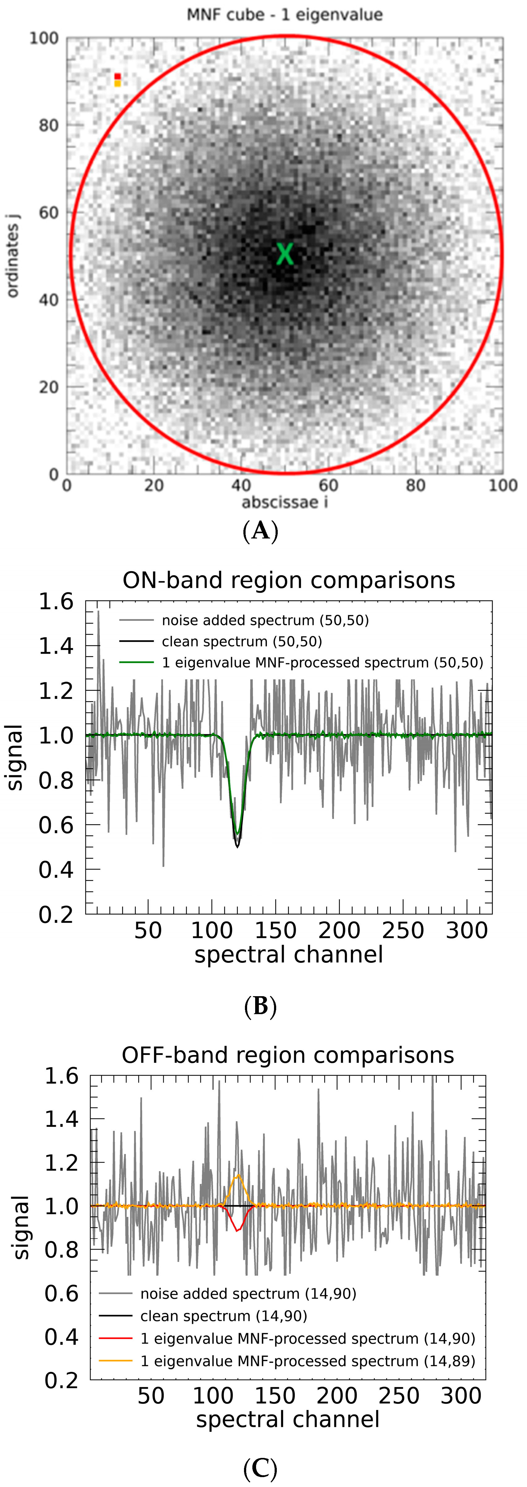
3.2.2. Reconstructed Data Coherence and Scientific Case

The same synthetic dataset also allows for checking for eventual biases in the spatial distribution of spectral features in MNF-reconstructed data since it is possible to verify if the radial gradient of β is preserved after the processing. To this purpose, we evaluate the β equivalent width for both the noise-added initial cube (β_noisy) and the MNF-processed one (β_MNF), reconstructed with N_e = 4 as in Section 3.2.1. The comparison with the nominal noise-free band area, β_clean, quantifies the absorption bias for each spectrum before and after MNF application. Once averaged over coronal regions of different radius, which share the same values of β_clean, we obtain the bias profiles $\overline{{\beta }_{noisy}-{\beta }_{clean}}$ and $\overline{{\beta }_{MNF}-{\beta }_{clean}}$ shown in Figure 4. The mean values are very close to 0 for all β_clean values (black dashed curve), indicating that no bias emerges on average and that the reconstructed data are spatially coherent with the original ones. The spread of values associated with both profiles (shaded areas) is indicative of the band area uncertainties, which appear, of course, reduced in the MNF case. The large spread at small values of β_clean is expected due to the presence of the gradient, which makes the band comparable to the noise as the boundaries of the red circle are approached.

The tests described here and in the previous section shed light on the possible performances and limitations of MNF processing on NOMAD LNO data. In particular, we have seen how eventual MNF-induced spectral artifacts can only be statistically removed by adopting a suitable number of eigenvalues. As a consequence, a smaller N_e yielding a more efficient noise reduction can only be adopted when dealing with average trends of ubiquitous species’ spectral signatures. This is the case, for example, of gases like CO₂, H₂O, and CO, which are widespread in the Martian atmosphere, and, hence, the accuracy of their geographical or climatological mapping would benefit from the MNF application.

By definition of the MNF, increasing N_e results in enhanced fluctuations, which can progressively embed the spectral artifacts, in fact removing them, as is evident from Figure 5A–E. The trend of artifact occurrence and SNR gain with respect to N_e is shown in Figure 5F. The overall monotone decrease in the two curves is a general property of the MNF that allows us to select the number of eigenvalues on the basis of the purpose of the analysis. It is indeed possible to decrease the spectral artifacts’ significance at the cost of reducing the SNR gain. This enables us to more reliably deal with species less statistically represented in the dataset, hence requiring more eigenvalues for a robust spectral information reconstruction (e.g., CO₂ ice; see Section 4.1).

In summary, we can identify two main regimes of N_e, whose threshold value needs to be determined case by case: (1) smaller values providing a high SNR gain and mostly useful for the investigation of spectral features that are more widespread in the dataset and (2) larger values high enough to make the spectral artifacts irrelevant for the analysis, yielding a moderate SNR gain but enabling the possibility to better characterize non-ubiquitous features (see Section 4.3.1).

4. Results: Application to LNO Nadir Data

As described in Section 2.1, LNO acquires data in spectral orders about 22 cm⁻¹ wide, each covering different species’ spectral signatures related to gases, aerosols, and ices (an overview of the spectral ranges and features covered by all orders can be found in [23]). The SNR performance worsening caused by the cryocooler removal is, of course, more significant for all spectral ranges where the Martian radiance level is low. This is particularly evident with orders 149–165, covering the wavelength range of 2.58–2.70 μm, which is affected by strong CO₂ and H₂O absorption bands, and with orders 119–136 (3.24–3.74 μm), in which the instrumental performances are so reduced to yield an average SNR of <2.

4.1. Methane and Other Trace Gases

The wavelength range covered by orders 134–136 (3.24–3.32 μm) is diagnostic for methane, whose presence on Mars is still debated nowadays. Recent TGO limb measurements from both ACS and NOMAD instruments did not succeed in detecting this gas [24], providing constraints on its airborne abundance (upper limit of 20 ppt for altitudes above 10 km [25]). On the other hand, in situ measurements from the Curiosity rover’s SAM-TLS spectrometer suggest that it could be circumscribed at low altitude and released during nighttime seepage events happening in Gale crater [16]. In this context, LNO nadir observations, contrary to limb viewing, offer a unique opportunity for methane detection, being sensitive to the whole atmospheric column down to the surface. Therefore, these observations would definitely benefit from the application of a noise-reduction technique such as the MNF, which could potentially reduce their noise and expand the possibilities for their investigation.

However, it is worth stressing that the detection of methane lines with the abundances described above would require a SNR of the order of thousands, way beyond the maximum value achievable thanks to the MNF gain (see Figure 5F). Moreover, in these orders, the SNR is so low that the spectral calibration described in Section 2.2 is not applicable since no solar or gaseous lines can be identified. In turn, a non-reliable wavenumber calibration can alter the statistical behavior of the signal, thereby preventing the MNF’s capability of identifying spectral correlations in the observations.

The above problems, related to both the spectral calibration and the too high SNR requirement for the identification of faint gaseous lines, are not specific for methane only but apply, in general, to other spectroscopically weak species (like HCl and HDO, covered by order 121). As a consequence, the application of the MNF to these data, at least with the assumptions made here, unfortunately does not provide a significant enhancement for the detection and analysis of Martian trace gases.

4.2. Widespread Species

On the other hand, MNF appears more useful in the LNO orders covering the solar-reflected part of the spectrum, at wavelengths lower than 2.7 μm (orders above 165). In this case, the observations are characterized by an overall higher signal, which, in most cases, allows for robust spectral calibration. Their SNR spans from very low (less than 2) to moderate/high (about 70), hence providing a good framework to test the MNF with different regimes of noise.

For our analysis, we focus on LNO data in orders 168 and 189 acquired from March 2018 to February 2023 (more than 420,000 spectra for each order, covering several TGO orbits), hence from the second half of Mars year 34 (MY34) to the beginning of MY37 (see

Table 2. LNO spectral orders selected for the MNF application.

LNO Order	Spectral Features	λ Range (μm)	wn Range (cm−1)	Mean SNR
168	H2O/CO2	2.627–2.648	3776.32–3806.49	8
189	CO2 ice/CO	2335–2353	4248.36–4282.30	10

). These orders are diagnostic of different spectral features related to both gases and surface ice. Order 168 encompasses several gaseous absorption lines of H₂O as well as some weaker ones of CO₂,while order 189 covers different CO gas absorption lines and a CO₂ ice absorption band (see Section 4.3.1). In particular, the latter has been recently investigated to spot surface frost on Mars polar caps and high-altitude CO₂ ice clouds in sporadic LNO observations [23]. High-latitude observations are particularly interesting for the detection of CO₂ ice on the surface, although their SNR is strongly affected by the poor polar illumination conditions. Therefore, the application of the MNF is particularly desirable to achieve an enhancement of their SNR.

In Section 4.3, we take as an example order 189 data to present updated methods (that also apply to order 168) for selecting N_e with LNO data and show how this number relates to the scientific goals of the investigation.

4.3. Concept for Eigenvalues Selection

For the purpose of MNF application, we arrange LNO data of a given order as a stacked three-dimensional array, keeping only those spectra in which the radiometric and spectral calibrations are reliable (Figure 6A). Since no dark measurements are available (background subtraction is performed onboard), we build the noise dataset from a series of LNO spectra acquired in nightside, where no signal from the target is present. For LNO data, this approach is expected to be more reliable than noise estimations based on the signal dataset itself, which retain dependences on the spatial distribution of the signal (e.g., [26]).

Such a setting allows for easy computation of both the signal and noise statistics required by the MNF. As already discussed in the synthetic dataset testing (Section 3.2), a way to check for the eventual presence of spectral artifacts induced by the technique is required. We achieve this by appending to the data cube a further column randomly filled with spectra from the noise cube. Since we know that this control column contains only noise, it can be used for probing the emergence of unwanted signals after the MNF application. As in the synthetic dataset case, a too small N_e value makes some non-negligible spectral features appear in the control column, which are clearly larger than the continuum fluctuations (i.e., having SNR values larger than 1). The high-gain N_e selection approach described in Section 3.2.2 is not equally applicable with the high-resolution LNO data since these are widespread with absorption lines of variable depth and intensity that prevent a robust definition of the spectral fluctuations of the continuum (the γ quantity in Section 3.2.2). Therefore, in order to ensure that the features in the control column become statistically negligible, in this case, we increase the number of eigenvalues until the average SNR over the whole column drops below 1. This threshold (referred to as “threshold 1” from now on) yields quite high SNR gain and makes the spectral artifacts statistically meaningless within the reconstructed noise. It represents the minimum number N_min of eigenvalues to be adopted for a reliable reconstruction of the data (N_min = 6 and 7 for LNO orders 168 and 189, respectively, yielding an average SNR gain of about 10 in both cases).

However, the MNF being a PC-based technique (Section 3.1), in the case of statistically less-represented spectral features (e.g., low frequency modulations pertaining to surface mineralogy and aerosols), whose presence in the dataset is non-uniform and less correlated with other widespread ones, the information content is likely spread over several eigenvectors, and, hence, it is possibly lost if threshold 1 is adopted. Therefore, we also define a more conservative threshold (that we call “threshold 2”) based on the change in the spectral shape between two successive reconstructions with N_e and N_e + 1 eigenvalues. Indeed, the average spectral residual δ of adjacent N_e and N_e+1 reconstructed spectra is a monotonically decreasing function of N_e for N_e > N_min, while the spectral fluctuation ε of the N_e reconstructed observation is an increasing function. The optimal number of eigenvalues is then obtained as the maximum N_e value for which δ > ε. As we will see in the next section and in Section 5.3, such a method is mostly effective if applied to subsets of the data in which the investigated spectral feature is already expected to be present more frequently. This enhances its statistical significance and allows a reliable reconstruction of the spectral information with a limited number of eigenvalues. This is the case, for example, of the CO₂ ice on the surface of Mars, which is mostly located on the planet’s polar caps.

4.3.1. Thresholds 1 and 2 Case Studies

As mentioned above, the choice of which threshold is to be preferred depends on the scientific purpose of the analysis. Taking into account order 189 data as an example, if the investigation is aimed at seasonally quantifying the abundance of gaseous CO, threshold 1 might be preferred. Indeed, CO is produced by the photolysis of CO₂, which is predominant in the Martian atmosphere, and is therefore a species widespread on the whole planet with an abundance (800 ppm on average) that makes it quite easily retrievable from remote sensing observations (e.g., [27,28,29,30,31,32]). Narrow lines belonging to the CO first overtone band at 4256.2 cm⁻¹ (first transition of the P branch) and 4263.8, 4267.5, 4271.2, 4274.7, and 4278.2 cm⁻¹ (first five transitions of the R branch) are detectable in LNO order 189 nadir data, even if the limited SNR can often make their identification difficult at the single spectrum level. Instead, the second transition of the P branch, at 4252.3 cm⁻¹, is mostly buried in the nominal noise of the observations. In Figure 7A, we give an example of a comparison between a sample mid-latitude’s order 189 spectrum (black line; note the modulation induced by the reflectance factor calibration discussed in Section 2.2) and the corresponding MNF-processed spectrum reconstructed with 7 eigenvalues (red line). A CO absorption simulation performed with the MITRA radiative transfer tool [6,28] is also shown as a reference for the position of CO absorption lines (in cyan). From the image, it is evident how the reduced noise fluctuations in the reconstructed spectrum allow for a more accurate measurement of these signatures and even make the 4252.3 cm⁻¹ line detectable. The same enhancement is also true for gaseous H₂O and CO₂ absorption lines falling in the range of order 168 (shown in Figure 7B) after MNF processing with N_e = 6. CO₂ lines in particular are very weak (owning to hot band 2ν₁ − ν₁) and mostly superimposed to the stronger H₂O ones (mainly part of water ν₁ and ν₃ fundamental bands). Nevertheless, after the MNF application, it is possible to identify lines as faint as the CO₂ line at 3792.0 cm⁻¹, only 0.8 cm⁻¹ away from the center of the 2ν₂ H₂O line at 3792.8 cm⁻¹.

Different is the case of CO₂ ice, whose 4255 cm⁻¹ absorption band (replicated at 4278 cm⁻¹ by the LNO response function; see Section 2.2 and also [23]) is as large as the whole order 189 spectral range (see cyan lines in Figure 7C,D offset for clarity). In the NOMAD dataset, it is mostly observed on the polar caps or in specific locations pertaining to either residual nighttime surface frost or high-altitude CO₂ ice clouds [23]. For the above reasons, its spectral correlation within the whole dataset is smaller than that of gaseous CO, such that to avoid loss of information in the MNF reconstruction, it would require a very large number of eigenvalues, yielding no SNR gain and hence making the algorithm application worthless, even if threshold 2 is selected in this case. An example of this behavior is given in Figure 7C, in which a LNO spectrum taken on the Martian South pole and showing an evident CO₂ ice absorption (black line) is reconstructed taking into account MNF statistics’ eigenvalues computed from the whole global dataset of order 189. The blue, green, and red spectra in Figure 7C, obtained by adopting very different N_e values (7, 100, and 300, respectively), show how the information related to the ice band spectral shape is correctly preserved only with N_e = 300, while lower eigenvalues provide reconstructed spectra with underestimated absorptions at both 4255 and 4278 cm⁻¹. Indeed, considering the 4278 cm⁻¹ band as an example, the blue and green spectra provide equivalent widths that are only 40% and 65% of the nominal LNO ones, while a 90% value is exceeded with the red spectrum.

Better results in terms of SNR gain can be achieved if we select only observations falling in a latitude range that encompasses the polar caps (e.g., latitudes larger than ±50°). The significance of exposed ice features in this subset is of course larger, and, in this case, more than 99% of the observations are reliably reconstructed (i.e., threshold 2 condition is met) with N_e ≤ 13 (Figure 7E), allowing a significant SNR gain for the CO₂ ice feature investigation. With such an approach, taking into account the same South polar ice spectrum as in Figure 7C, we show in Figure 7D how it can now be reconstructed with only 8 eigenvalues. The equivalent width of the 4278 cm⁻¹ band is now about 95% of the nominal one, demonstrating a robust preservation of the ice spectral shape with enhanced precision.

To summarize, in general, threshold 1 can be used to deal with ubiquitous spectral features and can be applied to the full dataset of a given order, yielding an average minimum number of eigenvalues that ensures a high SNR gain. On the other hand, threshold 2 is the best way to proceed if a robust reconstruction of spectral signatures with weaker spectral correlation is needed, at the cost of having to deal with limited subsets of data at once and a potentially reduced SNR gain.

5. Discussion

In the previous section, we have seen how the MNF allows for the enhancement of the average SNR of orders 168 and 189 by about one order of magnitude. This improvement is expected to enable more accurate retrievals of physical quantities in the study of global or seasonal trends (for example, water vapor and CO abundances), which are achievable through dedicated radiative transfer investigations capable of correctly dealing with all the physical and instrumental parameters involved (e.g., surface albedo, airborne dust content, illumination and observing geometry, AOTF, and Blaze functions). Such an analysis is beyond the scope of the present paper, but in the next sections, we discuss how the increased data SNR is expected to improve the evaluation of these trends.

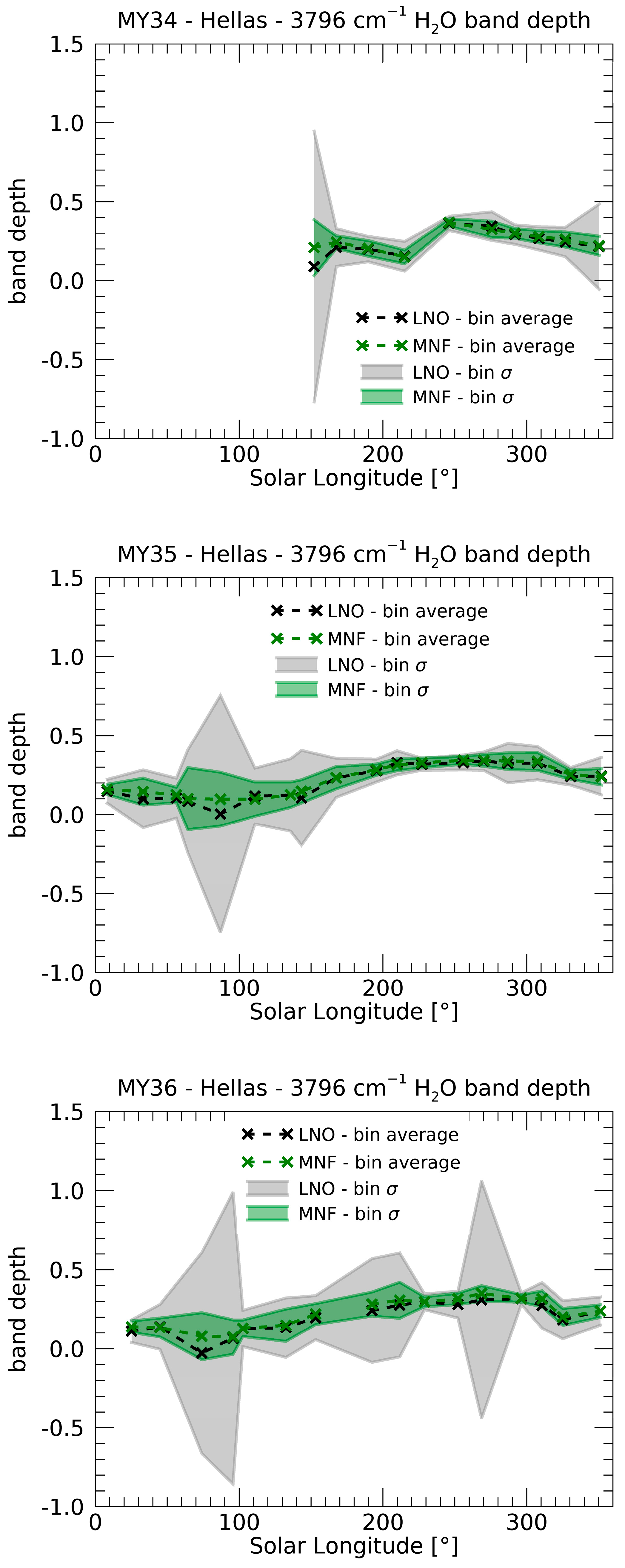
5.1. Example of a Seasonal Gas Trend: Water Vapor

As far as order 168 is concerned, the improvement in the accuracy of MNF processing can be quantified by computing the equivalent width of one of the covered H₂O absorption lines. The band depth correlates with the column density of water vapor in the atmospheric column and is affected by the observing conditions, in particular by altimetry. The strongest lines in the order 168 range, at 3779.5, 3784.6, 3796.4, and 3801.4 cm⁻¹, are all pertaining to the ν₃ fundamental stretching band and are overlayed with other weaker H₂O and CO₂ lines. Here, we focus on the one centered at 3796.4 cm⁻¹ (see Figure 7B) and separate the MY34, 35, and 36 data to derive the respective seasonal trends. In order to mitigate the band depth dependence on altimetry, we consider only those observations related to the Hellas basin, characterized by the lowest surface altitudes on Mars. We then compare the original and the MNF-processed band depths (threshold 1 is adopted; see Section 4.1 and Section 4.2), averaging them in bins of Ls of 20°, wide enough to homogeneously cover all seasons in the three Mars years. In the results shown in Figure 8, it is evident how some bins of the original dataset (grey shaded areas) are characterized by very large standard deviations (e.g., 150° < Ls < 170° in MY34 and 60° < Ls < 160° in MY35; 50° < Ls < 100°, 150° < Ls < 230°, and 260° < Ls < 300° in MY36). In general, the average values (black and green dashed lines in the figure) are not affected by the MNF processing, but it is evident how their uncertainties are consistently reduced after the MNF application, up to 90%. Such an enhancement helps greatly improve the accuracy of these seasonal trends, in fact, enabling the possibility of exploiting LNO nadir data to study water vapor columnar densities down to the surface.

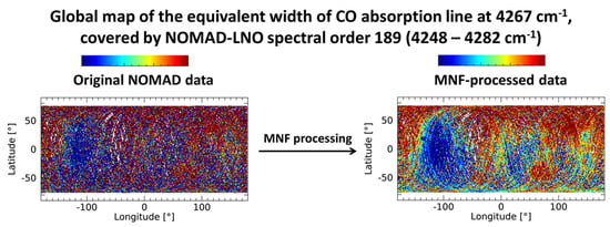
5.2. Example of Global Mapping: The Case of Gaseous CO

Several CO absorption lines of variable intensity fall within the order 189 spectral range. As we have seen in Section 4.3.1, the strongest ones are found at 4252.3, 4256.2, 4263.8, 4267.5, 4271.2, 4274.7, and 4278.2 cm⁻¹ (see cyan spectrum in Figure 7A) and are all part of the R branch of the ν = 0–2 band of ¹²C¹⁶O. As a benchmark for our analysis, we selected the 4267 cm⁻¹ line since it is the strongest one close to the center of the order, hence less affected by instrumental modulations (Section 2.2). In order to test the SNR enhancement induced by the MNF, we build longitude-latitude global maps of the line’s equivalent width (one for the initial dataset and another for the dataset processed with threshold 1), providing a proxy for the CO-integrated column. The best approach to comparing these maps would be to select ensembles of data as homogenous as possible, that is, considering observations related to narrow ranges of solar longitude (Ls), local time, incidence, and phase angle. However, the spatial and temporal coverage of LNO observations would only allow comparing very limited regions or periods of time (Section 2.1). For this reason, we bin all data in steps of 1° × 1° of longitude and latitude, regardless of the season, local time, and observing geometry, at the cost of increased fluctuations among adjacent bins. As in the case of water vapor (see previous section), the CO band depth variation is expected to be mostly driven by the altimetry of the surface, to which the total column is anti-correlated. This behavior is evident in Figure 9A,B, showing, respectively, a simulation of the CO-integrated column obtained from the Mars Climate Database (version 6.1, [35]) and the averaged LNO observations’ surface altimetry obtained from the Mars Orbiter Laser Altimeter (MOLA) data [36]. The equivalent width maps related to the initial and processed datasets are shown in Figure 9C,D. In Figure 9C, a dichotomy between regions of high and low width (corresponding to low and high altimetry regimes; see Figure 9A,B, respectively) is barely appearing but largely scattered by the noise. On the other hand, the contrast is enhanced in the MNF-processed map (Figure 9D), showing a more definite correspondence with both the MCD CO column map (Figure 9A) and the LNO surface altimetry one (Figure 9B). This is also confirmed by the scatter plots in Figure 9E,F, showing how, after the application of the MNF, the spread between the MCD-predicted densities and the computed equivalent widths is greatly reduced.

It is indeed possible to better identify the increased CO band depth (i.e., larger columnar abundance) associated with the northern lowlands of Arcadia (47°N, 175°W), Acidalia (49°N, 20°W), and Utopia Planitia (46°N, 119°E) as well as in the southern depressions of Argyre (50°N, 44°S) and Hellas Planitia (42°S, 70°E). Similarly, a particularly reduced CO column is observed, as expected, on the Tharsis volcanoes region (0°N, 110°W), which is characterized by the highest surface altitudes on the planet (see Figure 9B). It is interesting to note that the MNF-processed map in Figure 9D also allows to correctly spot the strongly depauperated CO column above both Olympus Mons (18°N, 134°W) and Elysium Mons (25°N, 147°E), whose peaks extend to about 20 and 13 km, respectively.

This test demonstrates how the characterization of ubiquitous spectral features (like the CO absorption lines considered here) can benefit from the application of the MNF. The enhanced SNR can be exploited to increase the accuracy in the retrieval of the most common Martian gaseous species’ abundance (e.g., CO₂, H₂O, and CO), in turn enabling more accurate estimates of their detection limits, seasonal trends, climatological cycles, and chemical patterns. For example, [38] recently exploited LNO nadir observations from orders 189 and 190 to derive the CO climatology across MY34 and MY35, demonstrating how these high-resolution data provide significant insights into our understanding of the Martian atmosphere. The application of the MNF would enhance the accuracy of the retrieved abundances, enabling a more fruitful comparison with other observations of Mars’ atmosphere and contributing to the improvement of climatological models.

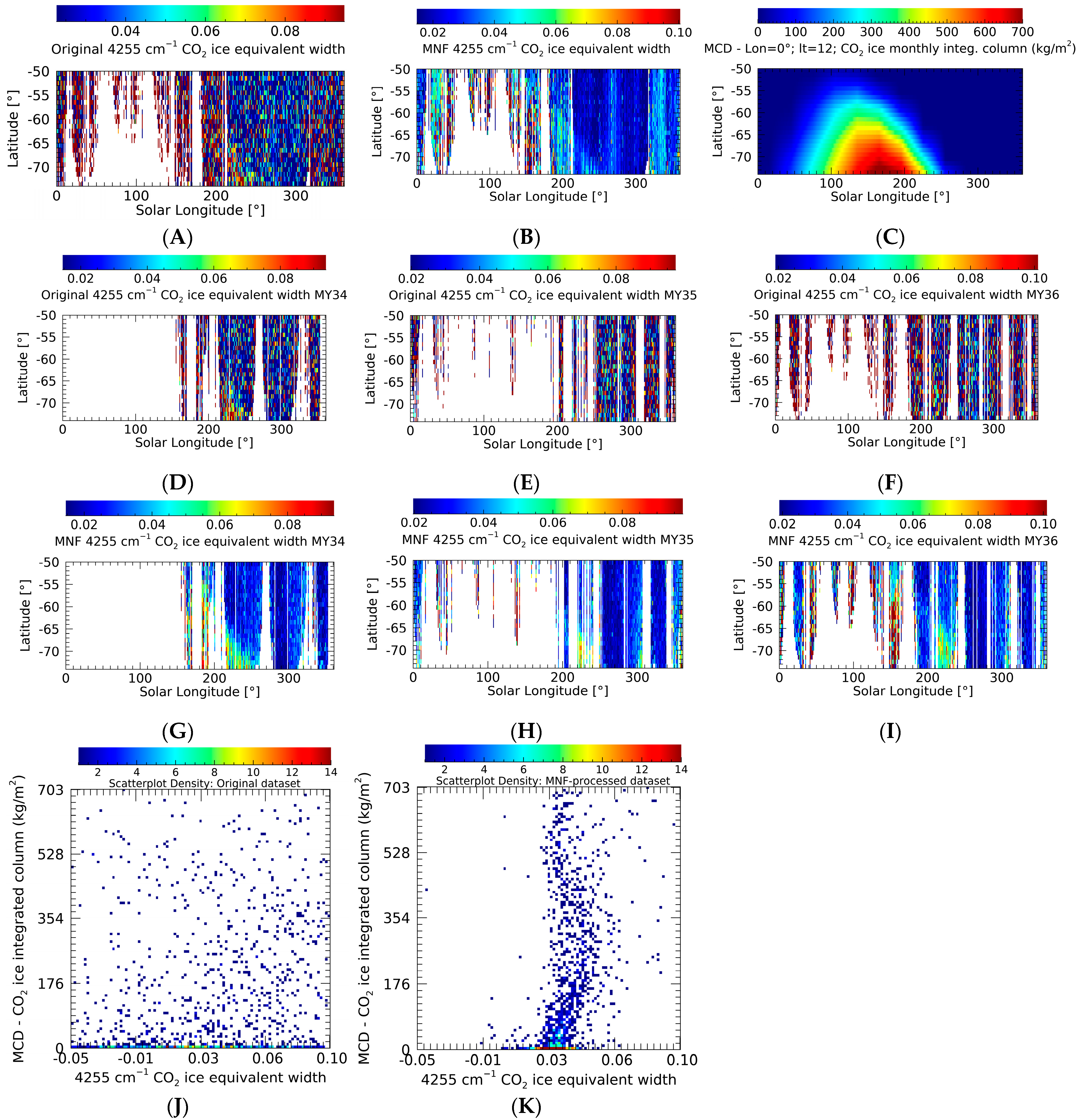
5.3. Example of Regional Mapping Features: The Case of CO₂ Ice

We now discuss the application of the MNF to a spectral feature that is less frequent in the dataset, that is, the CO₂ ice absorption band centered at 2.35 μm (4255 cm⁻¹). As already discussed in [23], this is quite a narrow and shallow combination band located in the 2.1–2.5 μm CO₂ ice transparency window. Being not a widespread feature, we adopt threshold 2 for eigenvalues’ selection (Section 4.1). Furthermore, as described in Section 4.3.1, we reduce the dataset in order to preserve the statistical significance of the ice feature and consider only observations limited to latitudes below 50°S, wide enough to encompass the maximum extension of the southern polar cap.

In this case study, an effective way to verify the MNF outcome is to investigate the seasonal trend of CO₂ ice condensation and sublimation phases, which define the outer boundary of the southern cap. For this purpose, we build Ls-latitude maps of the 2.35 μm equivalent width that we can compare to MCD simulations of the average Martian CO₂ ice monthly integrated column, as shown in Figure 10C.

The maps in Figure 10A,B contain data from all Martian years MY34, 35, and 36 averaged together in bins of 1° × 1° of Ls and latitude from the initial and MNF-processed datasets, respectively. The original data map displays an overall dichotomy of either large or small equivalent width values, but their distribution is quite noisy, resulting in polar cap edges that are barely detectable. On the other hand, in the MNF-processed map, the contrast between icy and non-icy terrains is enhanced, making the polar cap boundary much better identifiable. For example, this map agrees with the low ice content predicted by the climatological model at solar longitudes lower than 50° and larger than 300°, while the original data map does not. The main discrepancy between the MNF-processed map in Figure 10B and the MCD model in Figure 10C is seen at 190° ≤ Ls ≤ 210°, where the observed values are systematically lower. This is mainly due to a LNO coverage bias (Section 2.1), which makes the map bins not uniform in terms of observing conditions. In fact, in that Ls range, the South polar cap is characterized by its strongest longitudinal asymmetries in ice content (e.g., [39]). Such a behavior is evident in the scatter plots in Figure 10J,K, in which the MCD-derived densities are compared to the ice equivalent widths from the original and the MNF-processed observations, respectively. After the application of the technique, there is an increasing trend at low densities (less than about 200 kg/m²). However, this trend is lost for higher density values (related to the southernmost regions of the polar cap) due to the non-uniform coverage of LNO observations in this Ls range. This issue can be resolved once additional observations are available, allowing us to produce more homogenous datasets less affected by non-consistent spatial/temporal coverage of the observations. This would also enable the possibility to separate the data of future Mars years for investigating inter-annual differences in the ice seasonal trends. For example, a qualitative investigation of the inter-annual variations of the polar cap boundaries from the currently available dataset is shown in Figure 10D–I, related to the original and processed observations, respectively. The enhancement due to the MNF application is evident and highlights some differences, like, for example, a more equatorward cap boundary at Ls = 220° in MY36 with respect to MY34, demonstrating the potential of the technique even for the investigation of non-ubiquitous species in LNO nadir data.

6. Summary and Conclusions

In this study, we have investigated the possibility of increasing the SNR of TGO/NOMAD LNO infrared channel nadir data through the application of the Minimum Noise Fraction algorithm. A preliminary test on a synthetic dataset (Section 3) allowed us to better understand the expected performances of the technique as well as its intrinsic limitations, mostly related to the possible emergence of artifacts triggered by selection effects on the spectral fluctuations. In this way, we derive two statistically robust criteria to select the suitable number of eigenvalues for LNO data processing, specifically crafted to provide a trade-off between SNR gain and artifact mitigation. This number results in being dependent on the scientific purpose of the analysis: a small number of eigenvalues provides a high SNR gain and is the best option for the analysis of spectral features globally widespread in the considered dataset; on the other hand, a larger number of eigenvalues is desirable for non-ubiquitous or sporadic features, reducing the SNR gain but ensuring a more reliable reconstruction of the spectral information.

Some LNO orders, although very worthy of investigation (like, e.g., order 134, diagnostic of methane, or order 121, which covers HCl and HDO lines), are currently poorly spectrally calibrated due to the lack of spectral lines strong enough to drive wavenumber fine tuning, hence preventing a meaningful spectral covariance analysis for MNF processing. In any case, even if a reliable spectral calibration was available, the potential spectral features covered by these orders are so faint (e.g., methane absorption bands covered by order 134 would require a SNR of the order of thousands) that they would still be undetectable within the reduced noise obtained through the MNF processing (Section 4.1). On the other hand, we tested the MNF application to observations of LNO spectral orders 168 and 189 (Section 4), covering several H₂O and CO absorption lines and a broad CO₂ ice absorption band and encompassing both ubiquitous (H₂O and CO) and non-ubiquitous (CO₂ ice) cases. To verify the enhancement between the initial and processed datasets (Section 5), we compute equivalent widths for a H₂O line at 3976 cm⁻¹ (order 168), a CO line at 4267 cm⁻¹, and the CO₂ ice band peaked at 4255 cm⁻¹ (order 189), providing information on the respective column integrated densities. After the MNF application, uncertainties are reduced up to 90%, yielding an average SNR gain of about 10 for both orders. Such an enhancement even allows to identify a weak CO₂ absorption line (3972 cm⁻¹; part of the ν₂ν₃ ¹²C¹⁶O₂ hot band) that was fully masked by the noise in the initial order 168 observations, providing interesting perspectives in the application of the technique. We demonstrate that MNF processing is able to significantly improve the accuracy of H₂O and CO equivalent width maps. In particular, in the case of CO global mapping, the technique reveals the expected correlation with the Martian altimetry, which was only barely identifiable in the original dataset. Similarly, in applying MNF to CO₂ ice spectral features, we verify the enhanced detectability of the South polar cap boundary and its seasonal average behavior, allowing us to potentially compare its trend in different Martian years (MY34, 35, and 36). CO₂ and H₂O ices have been recently studied in NOMAD data, which detected both abundant surface deposits and thick clouds [23,40]. However, those analyses have been strongly affected by the observations’ SNR. The enhancement deriving from the MNF application would potentially enable the study of more localized or transient phenomena, like smaller and thinner frost deposits in shadowed craters’ rims or clouds characterized by lower optical depth.

The analyses presented in this paper demonstrate how the MNF algorithm can be applied to LNO nadir data to enhance their SNR, even if the processing needs to be tuned depending on the scientific purpose of the analysis, hence yielding a variable gain. Unavoidable constraints for further SNR improvements come from the sparse spatial and temporal coverage of LNO data due to the observing strategy that alternates the acquisition of different spectral orders (Section 2.1), in turn impacting the statistical significance of the spectral signatures that can be helpfully investigated.

References

1. Vandaele, A.; Neefs, E.; Drummond, R.; Thomas, I.; Daerden, F.; Lopez-Moreno, J.-J.; Rodriguez, J.; Patel, M.; Bellucci, G.; Allen, M.; et al. Science objectives and performances of NOMAD, a spectrometer suite for the ExoMars TGO mission. Planet. Space Sci. 2015, 119, 233–249. [Google Scholar] [CrossRef]
2. Nevejans, D.; Neefs, E.; Van Ransbeeck, E.; Berkenbosch, S.; Clairquin, R.; De Vos, L.; Moelans, W.; Glorieux, S.; Baeke, A.; Korablev, O.; et al. Compact high-resolution spaceborne echelle grating spectrometer with acousto-optical tunable filter based order sorting for the infrared domain from 22 to 43 μm. Appl. Opt. 2006, 45, 5191–5206. [Google Scholar] [CrossRef] [PubMed]
3. Formisano, V.; Angrilli, F.; Arnold, G.; Atreya, S.; Bianchini, G.; Biondi, D.; Blanco, A.; Blecka, M.; Coradini, A.; Colangeli, L.; et al. The Planetary Fourier Spectrometer (PFS) onboard the European Mars Express mission. Planet. Space Sci. 2005, 53, 963–974. [Google Scholar] [CrossRef]
4. Bertaux, J.-L.; Fonteyn, D.; Korablev, O.; Chassefière, E.; Dimarellis, E.; Dubois, J.; Hauchecorne, A.; Cabane, M.; Rannou, P.; Levasseur-Regourd, A.; et al. The study of the martian atmosphere from top to bottom with SPICAM light on mars express. Planet. Space Sci. 2000, 48, 1303–1320. [Google Scholar] [CrossRef]
5. Korablev, O.; Montmessin, F.; Trokhimovskiy, A.; Fedorova, A.A.; Shakun, A.V.; Grigoriev, A.V.; Moshkin, B.E.; Ignatiev, N.I.; Forget, F.; Lefèvre, F.; et al. The Atmospheric Chemistry Suite (ACS) of Three Spectrometers for the ExoMars 2016 Trace Gas Orbiter. Space Sci. Rev. 2017, 214, 7. [Google Scholar] [CrossRef]
6. Neefs, E.; Vandaele, A.C.; Drummond, R.; Thomas, I.R.; Berkenbosch, S.; Clairquin, R.; Delanoye, S.; Ristic, B.; Maes, J.; Bonnewijn, S.; et al. NOMAD spec-trometer on the ExoMars trace gas orbiter mission: Part 1—Design, manufacturing and testingof the infrared channels. Appl. Opt. 2015, 54, 8494–8520. [Google Scholar] [CrossRef]
7. Vandaele, A.C.; the NOMAD Team; Lopez-Moreno, J.-J.; Patel, M.R.; Bellucci, G.; Daerden, F.; Ristic, B.; Robert, S.; Thomas, I.R.; Wilquet, V.; et al. NOMAD, an Integrated Suite of Three Spectrometers for the ExoMars Trace Gas Mission: Technical Description, Science Objectives and Expected Performance. Space Sci. Rev. 2018, 214, 80. [Google Scholar] [CrossRef]
8. Jolliffe, I.T.; Cadima, J. Principal component analysis: A review and recent developments. Philos. Trans. R. Soc. A Math. Phys. Eng. Sci. 2016, 374, 20150202. [Google Scholar] [CrossRef]
9. Green, A.A.; Berman, M.; Switzer, P.; Craig, M.D. A Transformation for Ordering Multispectral Data in Terms of Image Quality with Implications for Noise Removal. IEEE Trans. Geosci. Remote Sens. 1988, 26, 65–74. [Google Scholar] [CrossRef]
10. Boardman, J.W.; Kruse, F.A. Automated Spectral Analysis: A Geological Example Using AVIRIS Data, North Grapevine Mountains, Nevada, ERIM, Ed. In Proceedings of the 10th Thematic Conference on Geological Remote Sensing, San Antonio, TX, USA, 9–12 May 1994; pp. 407–418. [Google Scholar]
11. Lee, J.B.; Woodyatt, A.S.; Berman, M. Enhancement of High Spectral Resolution Remote-Sensing Data by a Noise-Adjusted Principal Components Transform. IEEE Trans. Geosci. Remote Sens. 1990, 28, 295–304. [Google Scholar] [CrossRef]
12. Amato, U.; Cavalli, R.M.; Palombo, A.; Pignatti, S.; Santini, F. Experimental Approach to the Selection of the Components in the Minimum Noise Fraction. IEEE Trans. Geosci. Remote Sens. 2009, 47, 153–160. [Google Scholar] [CrossRef]
13. Bjorgan, A.; Randeberg, L.L. Real-Time Noise Removal for Line-Scanning Hyperspectral Devices Using a Minimum Noise Fraction-Based Approach. Sensors 2015, 15, 3362–3378. [Google Scholar] [CrossRef]
14. Luo, G.; Chen, G.; Tian, L.; Qin, K.; Qian, S.-E. Minimum Noise Fraction versus Principal Component Analysis as a Preprocessing Step for Hyperspectral Imagery Denoising. Can. J. Remote Sens. 2016, 42, 106–116. [Google Scholar] [CrossRef]
15. Nielsen, A.A.; Larsen, R. Restoration of GERIS data using the maximum noise fractions transform. In Proceedings of the First International Airborne Remote Sensing Conference and Exhibition, Strasbourg, France, 11–15 September 1994; pp. 557–568. [Google Scholar]
16. Moores, J.E.; King, P.L.; Smith, C.L.; Martinez, G.M.; Newman, C.E.; Guzewich, S.D.; Meslin, P.; Webster, C.R.; Mahaffy, P.R.; Atreya, S.K.; et al. The Methane Diurnal Variation and Microseepage Flux at Gale Crater, Mars as Constrained by the ExoMars Trace Gas Orbiter and Curiosity Observations. Geophys. Res. Lett. 2019, 46, 9430–9438. [Google Scholar] [CrossRef]
17. Patel, M.R.; Antoine, P.; Mason, J.; Leese, M.; Hathi, B.; Stevens, A.H.; Dawson, D.; Gow, J.; Ringrose, T.; Holmes, J.; et al. NOMAD spectrometer on the ExoMars trace gas orbiter mission: Part 2—Design, manufacturing, and testing of the ultraviolet and visible channel. Appl. Opt. 2017, 56, 2771–2782. [Google Scholar] [CrossRef] [PubMed]
18. Thomas, I.R.; Vandaele, A.C.; Robert, S.; Neefs, E.; Drummond, R.; Daerden, F.; Delanoye, S.; Depiesse, C.; Ristic, B.; Mahieux, A.; et al. NOMAD instrument—Part II: The IR channels—SO and LNO. Opt. Express 2016, 24, 3790–3805. [Google Scholar] [CrossRef] [PubMed]
19. Liuzzi, G.; Villanueva, G.L.; Mumma, M.J.; Smith, M.D.; Daerden, F.; Ristic, B.; Thomas, I.; Vandaele, A.C.; Patel, M.R.; Lopez-Moreno, J.-J.; et al. Methane on Mars: New insights into the sensitivity of CH4 with the NOMAD/ExoMars spectrometer through its first in-flight calibration. Icarus 2019, 321, 671–690. [Google Scholar] [CrossRef]
20. Thomas, I.R.; Aoki, S.; Trompet, L.; Robert, S.; Depiesse, C.; Willame, Y.; Cruz-Mermy, G.; Schmidt, F.; Erwin, J.T.; Vandaele, A.C.; et al. Calibration of NOMAD on ESA’s ExoMars Trace Gas Orbiter: Part 2—The Limb, Nadir and Occultation (LNO) channel. Planet. Space Sci. 2022, 218, 105410. [Google Scholar] [CrossRef]
21. Chang, C.-I.; Du, Q. Interference and noise-adjusted principal components analysis. IEEE Trans. Geosci. Remote Sens. 1999, 37, 2387–2396. [Google Scholar] [CrossRef]
22. Gordon, C. A generalization of the maximum noise fraction transform. IEEE Trans. Geosci. Remote Sens. 2000, 38, 608–610. [Google Scholar] [CrossRef]
23. Oliva, F.; D’aversa, E.; Bellucci, G.; Carrozzo, F.G.; Lozano, L.R.; Altieri, F.; Thomas, I.R.; Karatekin, O.; Mermy, G.C.; Schmidt, F.; et al. Martian CO2 Ice Observation at High Spectral Resolution with ExoMars/TGO NOMAD. J. Geophys. Res. Planets 2022, 127, 7083. [Google Scholar] [CrossRef] [PubMed]
24. Korablev, O.; The ACS and NOMAD Science Teams; Vandaele, A.C.; Montmessin, F.; Fedorova, A.A.; Trokhimovskiy, A.; Forget, F.; Lefèvre, F.; Daerden, F.; Thomas, I.R.; et al. No detection of methane on Mars from early ExoMars Trace Gas Orbiter observations. Nature 2019, 568, 517–520. [Google Scholar] [CrossRef] [PubMed]
25. Montmessin, F.; Korablev, O.I.; Trokhimovskiy, A.; Lefèvre, F.; Fedorova, A.A.; Baggio, L.; Irbah, A.; Lacombe, G.; Olsen, K.S.; Braude, A.S.; et al. A stringent upper limit of 20 pptv for methane on Mars and constraints on its dispersion outside Gale crater. Astron. Astrophys. 2021, 650, A140. [Google Scholar] [CrossRef]
26. Xue, T.; Wang, Y.; Chen, Y.; Jia, J.; Wen, M.; Guo, R.; Wu, T.; Deng, X. Mixed Noise Estimation Model for Optimized Kernel Minimum Noise Fraction Transformation in Hyperspectral Image Dimensionality Reduction. Remote Sens. 2021, 13, 2607. [Google Scholar] [CrossRef]
27. Encrenaz, T.; Fouchet, T.; Melchiorri, R.; Drossart, P.; Gondet, B.; Langevin, Y.; Bibring, J.-P.; Forget, F.; Bézard, B. Seasonal variations of the martian CO over Hellas as observed by OMEGA/Mars Express. Astron. Astrophys. 2006, 459, 265–270. [Google Scholar] [CrossRef]
28. Krasnopolsky, V.A. Long-term spectroscopic observations of latitudinal and seasonal variations of O2 dayglow and CO on Mars. Icarus 2006, 190, 93–102. [Google Scholar] [CrossRef]
29. Modak, A.; López-Valverde, M.A.; Brines, A.; Stolzenbach, A.; Funke, B.; González-Galindo, F.; Hill, B.; Aoki, S.; Thomas, I.; Liuzzi, G.; et al. Retrieval of Martian Atmospheric CO Vertical Profiles from NOMAD Observations During the First Year of TGO Operations. J. Geophys. Res. Planets 2023, 128, 7282. [Google Scholar] [CrossRef]
30. Rosenqvist, J.; Drossart, J.P.; Combes, M.; Encrenaz, T.; Lellouch, E.; Bibring, J.P.; Erard, S.; Langevin, Y.; Chassefiere, E. Minor constituents in the Martian atmosphere from the ISM/Phobos exper-iment. Icarus 1992, 98, 254–270. [Google Scholar] [CrossRef]
31. Sindoni, G.; Formisano, V.; Geminale, A. Observations of water vapour and carbon monoxide in the Martian atmosphere with the SWC of PFS/MEX. Planet. Space Sci. 2011, 59, 149–162. [Google Scholar] [CrossRef]
32. Smith, M.D.; Wolff, M.J.; Clancy, R.T.; Murchie, S.L. Compact Reconnaissance Imaging Spectrometer observations of water vapor and carbon monoxide. J. Geophys. Res. Planets 2009, 114, 3288. [Google Scholar] [CrossRef]
33. Oliva, F.; Geminale, A.; D’Aversa, E.; Altieri, F.; Bellucci, G.; Carrozzo, F.; Sindoni, G.; Grassi, D. Properties of a Martian local dust storm in Atlantis Chaos from OMEGA/MEX data. Icarus 2018, 300, 1–11. [Google Scholar] [CrossRef]
34. Flanner, M.G.; Zender, C.S.; Randerson, J.T.; Rasch, P.J. Present-day climate forcing and response from black carbon in snow. J. Geophys. Res. Atmos. 2007, 112, D11202. [Google Scholar] [CrossRef]
35. Millour, E.; Forget, F.; Spiga, A.; Vals, M.; Zakharov, V.; Montabone, L.; Lefèvre, F.; Montmessin, F.; Chaufray, J.-Y.; López-Valverde, M.A. The Mars Climate Database (MCD version 6). In Proceedings of the EPSC-DPS Joint Meeting, Geneva, Switzerland, 15–20 September 2019. [Google Scholar]
36. Smith, D.E.; Zuber, M.T.; Frey, H.V.; Garvin, J.B.; Head, J.W.; Muhleman, D.O.; Pettengill, G.H.; Phillips, R.J.; Solomon, S.C.; Zwally, H.J.; et al. Mars Orbiter Laser Altimeter: Experiment summary after the first year of global mapping of Mars. J. Geophys. Res. Planets 2001, 106, 23689–23722. [Google Scholar] [CrossRef]
37. D’Aversa, E.; Oliva, F.; Altieri, F.; Sindoni, G.; Carrozzo, F.G.; Bellucci, G.; Forget, F.; Geminale, A.; Mahieux, A.; Aoki, S.; et al. Vertical distribution of dust in the martian atmosphere: OMEGA/MEx limb observations. Icarus 2022, 371, 114702. [Google Scholar] [CrossRef]
38. Smith, M.D.; Daerden, F.; Neary, L.; Khayat, A.S.J.; Holmes, J.A.; Patel, M.R.; Villanueva, G.; Liuzzi, G.; Thomas, I.R.; Ristic, B.; et al. The climatology of carbon monoxide on Mars as observed by NOMAD na-dir-geometry observations. Icarus 2021, 362, 114404. [Google Scholar] [CrossRef]
39. Langevin, Y.; Bibring, J.; Montmessin, F.; Forget, F.; Vincendon, M.; Douté, S.; Poulet, F.; Gondet, B. Observations of the south seasonal cap of Mars during recession in 2004–2006 by the OMEGA visible/near-infrared imaging spectrometer on board Mars Express. J. Geophys. Res. Planets 2007, 112, 2841. [Google Scholar] [CrossRef]
40. Lozano, L.R.; Karatekin, O.; Dehant, V.; Bellucci, G.; Oliva, F.; D’aversa, E.; Carrozzo, F.G.; Altieri, F.; Thomas, I.R.; Willame, Y.; et al. Evaluation of the Capability of ExoMars-TGO NOMAD Infrared Nadir Channel for Water Ice Clouds Detection on Mars. Remote Sens. 2022, 14, 4143. [Google Scholar] [CrossRef]
Figure 1. (A) Structure of the clean (devoid of noise) synthetic data cube used for MNF tests, displayed on spectral channel 120. The red circle indicates the region where a spectral feature centered on this channel is present with a radial gradient. (B) Same as in panel (A) but with random Gaussian noise added in order to simulate a SNR = 5. (C) Noise cube for the noise covariance matrix computation of the MNF. (DF) Comparison between the spectra selected on the colored Xs in panel (A) (colored lines) and the corresponding spectra in panel (B) (grey lines).
Remotesensing 15 05741 g001
Figure 2. (A) MNF-processed data cube reconstructed with only 1 eigenvalue. (B) Comparison between the spectra on the green X in panel (A), related to the data cube in Figure 1B (grey line), to the clean cube in Figure 1A (black line), and to the MNF-reconstructed spectrum in panel (A) (green line). (C) Same comparison as in panel (B), but here referred to the red and orange pixels taken outside the red circle in panel (A).
Remotesensing 15 05741 g002
Figure 3. Comparison between the two sides of Equation (8), considering the + (panel (A)) and − signs (panel (B)) separately. The vertical dashed lines indicate the eigenvalue at which the quantities |μβ ± σβ| and |μγ ± σγ| become comparable within their uncertainties (see Section 3.2.1).
Remotesensing 15 05741 g003
Figure 4. Average differences between the synthetic dataset’s equivalent widths βnoisy and βMNF and the nominal band depth βclean (see Section 3.2.2), considering pixels of equal band depth. βmax on the abscissa indicates the maximum band depth of the clean dataset (Figure 1A). Uncertainties are shown as colored regions, while the black dashed line represents the average of β M N F β c l e a n ¯ at all band depths.
Remotesensing 15 05741 g004
Figure 5. Panels (AE) show the MNF-reconstructed spectra using 4, 20, 30, 50, and 60 eigenvalues, respectively. Panel (F) shows the trend of the artifacts occurrence as percent of the total number of considered pixels (black line and left ordinates) and the trend of the SNR (green line and right ordinates) as functions of Ne.
Remotesensing 15 05741 g005
Figure 6. (A) Spectral cube of order 189 data (incidence angle less than 90°) from March 2018 until February 2023, displayed at wavenumber k = 4265 cm−1 (i.e., the center of the order). (B) Noise cube for the application of the MNF, consisting of all order 189 observations having an incidence angle larger than 90°.
Remotesensing 15 05741 g006
Figure 7. (A) Comparison between a sample spectrum from LNO order 189 (black), its MNF-reconstructed counterpart (red), and a simulation of CO absorption (cyan) obtained with the MITRA RT tool [33]. (B) As in panel (A), but the black spectrum is related to LNO order 168, and the simulations are related to H2O (cyan) and CO2 (purple) absorptions. The inset zooms around the 3792 cm−1 CO2 absorption line to show how it becomes detectable after the MNF application. (C): sample order 189 South polar spectrum (black) compared to MNF spectra reconstructed with Ne = 7 (blue), 100 (green), and 300 (red). The eigenvalues here are computed considering the whole global LNO dataset in this order (see Section 4.3.1). A CO2 ice simulation with ice effective radius reff = 0.3 mm, performed with the SNICAR tool [34] and convolved with LNO response functions (hence also showing the CO2 ice “ghost” band at 4278 cm−1; see Section 4.3.1), is displayed as a reference in cyan and is offset for clarity. (D) As in panel (C), but the MNF-reconstructed spectra are provided for Ne = 1 (blue) and 8 (red), and the eigenvalues are computed from a high-latitudes dataset (Section 4.3.1). (E) Probability of having a reliable MNF reconstruction by adopting threshold 2 (see Section 4.1) in the case of the high-latitude dataset computation. The blue dashed line indicates Nmin = 7, derived from threshold 1, while the red dashed line indicates the value Ne = 13, corresponding to a 99% probability.
Remotesensing 15 05741 g007aRemotesensing 15 05741 g007bRemotesensing 15 05741 g007c
Figure 8. H2O 3796 cm−1 equivalent width of order 168 data, computed for observations falling in Hellas basin for MY34 (top), MY35 (middle), and MY36 (bottom), related to the original LNO data (black dashed line and grey shaded region) and the MNF-processed ones (green dashed line and shaded region). Ls bins of 20° are adopted for the computation.
Remotesensing 15 05741 g008
Figure 9. (A) MCD simulation of the CO-integrated column in kg/m2. (B) LNO order 189 data averaged surface altimetry in km (from MOLA data, [37]). (C) Equivalent width of the CO 4267 cm−1 absorption line computed on LNO order 189 original data. (D) Equivalent width of the CO 4267 cm−1 absorption line computed on the MNF-processed data (Ne = 7). (E) Density scatter plot of the quantities in panels (A,C). (F) As in panel (E), but here the quantities in panels (A,D) are being compared.
Remotesensing 15 05741 g009
Figure 10. (A) Equivalent width of the CO2 ice 4255 cm−1 absorption band computed on all MY34-35-36 LNO order 189 original data. (B) Same as in panel (A), but the equivalent width is computed on all MY34-35-36 MNF-processed data. (C) MCD simulation of the monthly integrated CO2 ice column in kg/m2. Panels (DF) are the same as panel (A), but the data are separated into MY34, 35, and 36, respectively. Similarly, panels (GI) show the MNF-processed equivalent width for MY34, 35, and 36, respectively. Panels (J,K) provide the density scatter plots between the quantities in panels (C)/(B) and (C)/(A), respectively, considering observations in the Ls range of 190°–210°.
Remotesensing 15 05741 g010