Article

Hyperspectral Image Assessment of Archaeo-Paleoanthropological Stratigraphic Deposits from Atapuerca (Burgos, Spain)

by
Berta García-Fernández
1,*,
Alfonso Benito-Calvo
2,*,
Adrián Martínez-Fernández
2,
Isidoro Campaña
3,
Andreu Ollé
4,5,
Palmira Saladié
4,5,
María Martinón-Torres
2 and
Marina Mosquera
4,5
1
Departamento de Ingeniería y Gestión Forestal y Ambiental, Escuela Técnica Superior de Ingeniería de Montes, Forestal y del Medio Natural, Universidad Politécnica de Madrid, Ciudad Universitaria, 28040 Madrid, Spain
2
Centro Nacional de Investigación sobre la Evolución Humana (CENIEH), Paseo Sierra de Atapuerca 3, 09002 Burgos, Spain
3
Departamento de Ecología y Geología, Facultad de Ciencias, Universidad de Málaga, Campo de Teatinos s/n, 29071 Málaga, Spain
4
Institut Català de Paleoecologia Humana i Evolució Social (IPHES-CERCA), Zona Educacional 4, Campus Sescelades URV (Edifici W3), 43007 Tarragona, Spain
5
Departament d’Història i Història de l’Art, Universitat Rovira i Virgili, Avinguda de Catalunya 35, 43002 Tarragona, Spain
*
Authors to whom correspondence should be addressed.
Heritage 2025, 8(6), 233; https://doi.org/10.3390/heritage8060233
Submission received: 16 May 2025 / Revised: 8 June 2025 / Accepted: 10 June 2025 / Published: 18 June 2025
(This article belongs to the Section Cultural Heritage)

Abstract

:
This paper proposes an experimental procedure based on hyperspectral imaging (HSI) combined with statistical classification for assessing archaeo-paleoanthropological stratigraphic deposits at the Gran Dolina site (TD10 unit), located in the Sierra de Atapuerca (Burgos, Spain). Representative spectral reflectance signatures were determined and analyzed using HSI measurements and statistical classification methods in natural light conditions across various capture distances. This study aims to characterize and quantify cave sediments by defining spectral models for feature classification and spectral similarity analysis, evaluating the strengths and limitations of spectral captures at this specific site. HSI technology enhances the analysis and identification of materials at an internationally recognized reference site for human evolution studies. Hyperspectral imaging assessment of archaeo-paleoanthropological stratigraphic deposits emerges as an innovative digital tool, revolutionizing the sustainable management of cultural heritage and environmental sciences by enabling advanced material identification and stratigraphic analysis.

1. Introduction

Spectroscopy has long served as a valuable quantitative tool in laboratory analysis, with various research methods evolving over time [1]. Recently, multiple scientific disciplines have adopted image spectroscopy, which is widely used as both a qualitative and quantitative research tool in mineralogy, agriculture, and environmental resource management. The hyperspectral imaging (HSI) system, especially in the visible infrared (VIR) and near infrared (NIR) ranges, provides extensive electromagnetic spectral data, capturing optical information of investigated samples. By combining high-spectral-range imaging with artificial intelligence analysis, HSI constitutes a non-destructive quality assessment method, enabling the analysis and identification of the spectral–spatial variation in materials or objects [2].
HSI data is derived from airborne, satellite, or near-field sensors. Airborne imaging spectroscopy (AIS) has applications in diverse fields such as soil erosion monitoring [3], riverbed morphodynamics [4], and rapid mapping of areas affected by natural disasters [5]. AIS also supports agronomic research, aiding in crop management and variability analysis [6], as well as landscape condition assessments, including changes in vegetation distribution due to climate change and land use shifts, a growing focus in landscape conservation worldwide [7,8,9].
In cultural heritage studies, multispectral and HSI techniques have proven effective for material classification [10,11]. MSI has facilitated the study of archaic cultures, where vegetation cover, soil composition, or depth-specific archaeological features pose significant challenges [12]. However, only recent studies have focused on detailed spectral analysis in geoarchaeology [13,14,15]. Hyperspectral imaging applied to sediment cores remains a developing tool, with the potential to enhance the understanding of paleo-environmental processes [13]. NIR spectroscopy, for instance, has been useful in stratigraphy studies, complementing wet chemical analyses in archaeological excavations [14]. New methods for analyzing archaeological airborne spectroscopy data, such as red edge inflexion point (REIP) and distribution fittings, further maximize remote-sensing data utilization [15].
While constraints still limit hyperspectral remote sensing in geological applications, prior AIS-based studies have shown promising results using processing techniques like principal component analysis and vegetation indices [16]. This technology has the potential to reveal environmental and geological features critical to the mining and environmental geology industries, with one of its significant applications being the production of geological maps that classify surface materials, including minerals and rocks.
The excavation of archaeological sites is key to understanding and disseminating the heritage of past societies, particularly in Paleolithic sites, where human activity left few structural imprints. In these contexts, precise identification and spatial documentation of archaeological elements within their stratigraphic context are essential for interpreting site formation processes.
Presently, excavation monitoring encompasses diverse methods, including detailed photographic documentation, topographic techniques (grids, total stations, and GNSS), and 3D mapping [17,18,19,20,21,22]. However, traditional techniques lack the capacity to analytically differentiate elements based on physical properties. Advances in image spectrometry, including high-capacity sensors, have enabled new areas of analysis and research [12,13,14,16].
This study applies hyperspectral imaging (HSI) technology to the identification and spectral characterization of stratigraphic contexts within the Paleolithic TD10 unit at the Gran Dolina site (Sierra de Atapuerca, Burgos, Spain). By expanding the analytical potential of HSI in an archaeo-paleoanthropological setting, the approach provides complementary data for the precise identification, classification, and mapping of geological and anthropogenic materials. In line with the emerging applications of HSI in cultural heritage research [11], this study highlights the technique’s growing relevance not only for material discrimination but also for supporting non-invasive preservation strategies in complex archaeological environments.

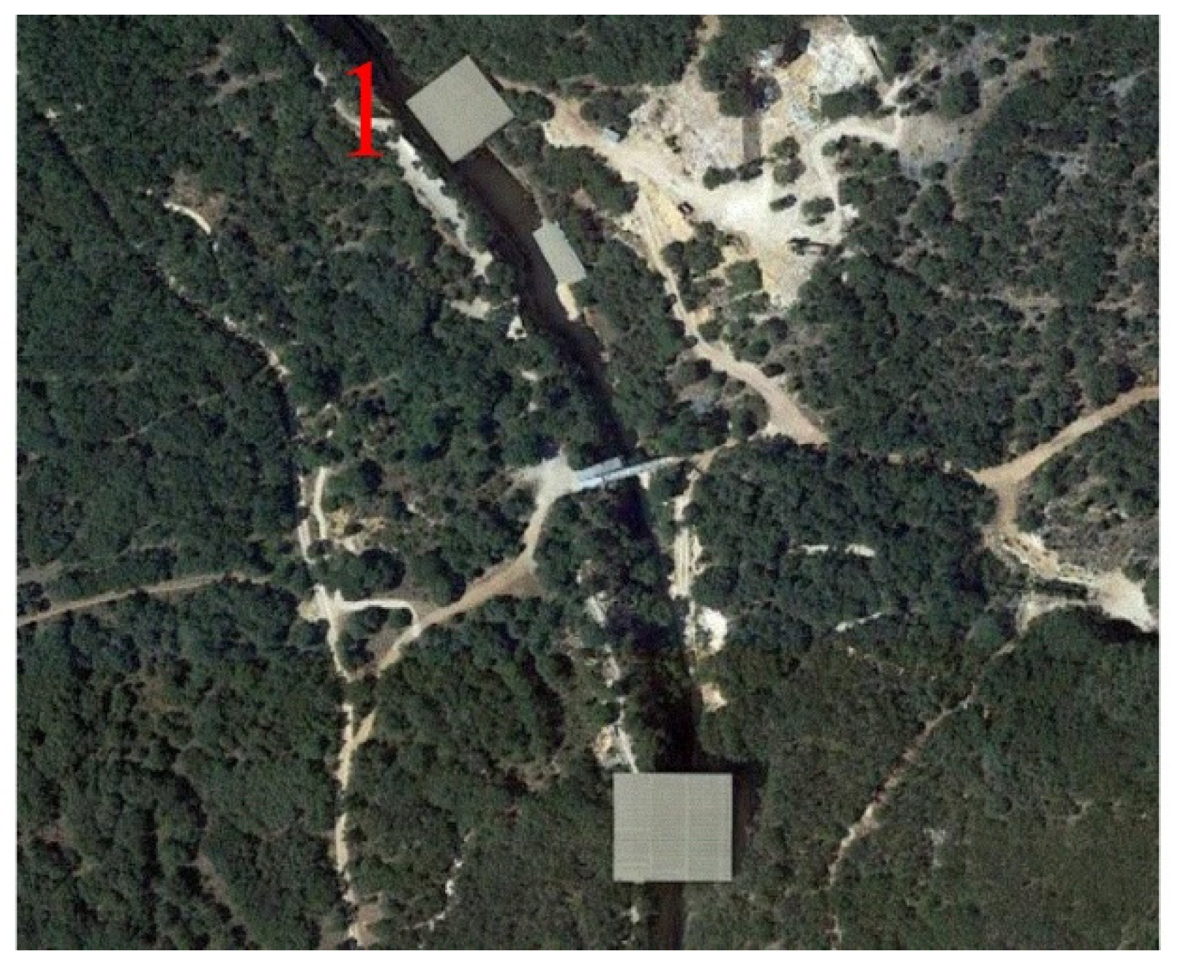
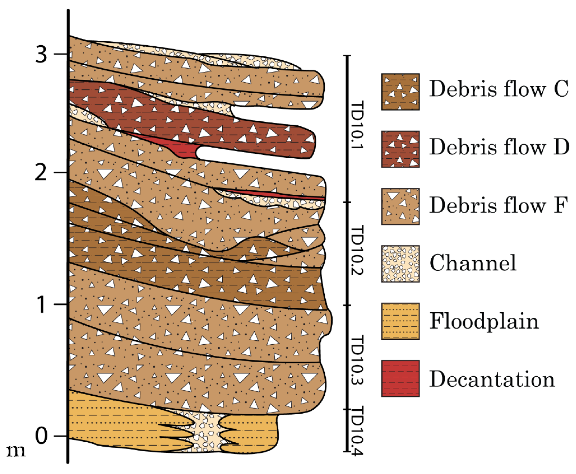
2. Background and Geoarchaeological Characteristics

The Gran Dolina site is located within the Sierra de Atapuerca, a low mountain range in northern Spain characterized by a folded Mesozoic sequence formed by an anticline structure. The bedrock in this area is composed predominantly of carbonates—mainly limestones and dolostones—of Late Cretaceous age, which serve as the host lithology for the karstic cave systems. These carbonate rocks provided the conditions necessary for the formation and long-term preservation of the cave sediments. Importantly, the region was not subjected to Quaternary glaciations, which has allowed the stratigraphic and archaeological records to remain relatively undisturbed over extended timescales. In the Sierra de Atapuerca (Burgos), Lower Paleolithic sites are preserved within sedimentary fills contained in a multilevel cave system [17,18], associated with Pleistocene fluvial levels imposed by the Arlanzón River [19,20]. The sediments containing archaeological remains were deposited by gravitational and water flow processes, forming breccias (composed of blocks and mud), gravel, sand, silt, and clay [22,23,24,25]. These sediments contain human fossils, stone tools (made of chert, quartzite, quartz, sandstone, and limestone), and faunal remains, spanning from the Early to the Middle Pleistocene [25,26,27,28]. Figure 1 shows an aerial view of the Atapuerca archaeological site (Burgos, Spain), with the location of Gran Dolina cave marked by a red number 1.
This study focuses on the Gran Dolina site, a 25 m thick cave infilling within the intermediate endokarst level [17], generated by the phreatic level associated with the Arlanzón fluvial terrace T3 during the Early Pleistocene [29]. The Gran Dolina sequence is divided into 12 lithostratigraphic units, numbered from bottom to top (TD1-TD11, with a later-defined TD8-9 unit) [22,23,24]. Units TD1 and TD2 are classified as cave interior facies, while TD3 to TD11 are categorized as cave entrance facies [23]. From TD4 to TD11, the cave was progressively filled by sediment inflow from a proximal entrance, continuing until complete silting occurred in the TD11 unit. These entrance facies are the result of sedimentary gravity flow processes—including debris fall, debris flow, and mud flow—as well as fluvial processes such as channel deposits, floodplain sediments, and decantation features [23]. The Gran Dolina site contains significant Early and Middle Pleistocene archaeo-paleontological levels [30,31,32], with documented lithic tools, as well as faunal and human remains [26,27,28]. Notably, the TD6 unit has yielded significant paleoanthropological evidence, including hominin remains, lithic tools, and faunal assemblages dated to approximately 0.8–0.9 million years ago, representing one of the earliest records of human presence in Western Europe [26]. In contrast, the TD10 unit—interpreted as a recurrent human occupation area or campsite dating to around 0.35 million years ago—has produced two extensive archaeological assemblages comprising over 30,000 lithic artifacts and approximately 99,000 faunal remains, underscoring the intensity and complexity of Middle Pleistocene hominin activity at the site [28]. The TD10 unit comprises a sequence of debris flow facies deposited from the main western entrance, with limited side entrances and occasional breakdown events [23,24]. This unit is further subdivided into four subunits, labeled from bottom to top as TD10.4 to TD10.1, each containing six described sedimentary facies (Table 1 and Figure 2) [23]. In Table 1, ‘grain’ refers to the fine sedimentary particles composing the matrix around larger elements, while ‘clast’ designates coarser stone fragments, generally within the pebble to cobble size range.
The basal subunit TD10.4 is composed of interbedded mud and gravel deposits, which have been interpreted as floodplain and channel sediments subsequently overlain by debris flow facies (facies F), as well as associated mudflow accumulations—reflecting a dynamic fluvio-gravitational depositional environment [23]. The channel facies, located centrally within the section, consist of approximately 70% centimeter-sized gravel and 30% mud. Mudflow and floodplain facies occupy the lateral parts of the section, mainly composed of mud with some gravel inclusions. Clasts observed near the walls are interpreted as having potentially fallen from the cave roof. These clasts were identified based on their large size—some exceeding one meter in diameter—and greater angularity. In some cases, surface features associated with karstic dissolution, characteristic of the cave interior, have also been observed on these clasts. Visual color assessments, performed according to the Munsell soil color charts, reveal that these facies exhibit a yellowish-red 5YR 5/8 hue, although some layers display a slightly more yellowish tint (Table 2). Additionally, phosphate crusts are present in certain layers of TD10.4, suggesting that the weathering process may be associated with the bat guano deposit found in TD9 [23]. Successive debris flow inputs from the primary western entry, with additional smaller secondary entries, formed subunits TD10.3, TD10.2, and TD10.1. TD10.3, measuring approximately 80 cm in thickness, contains at least two instances of debris flow facies F (Table 2 and Figure 2 and Figure 3). These are grain-supported clasts within a reddish-yellow 5YR 6/8 mud matrix, averaging 15 cm in diameter, with some clasts reaching 35 cm. Near-meter-diameter clasts observed within these layers suggest rockfalls from the cave roof, which may have enlarged existing entries or created new ones, as indicated by debris flow facies F from SE inputs [23]. Angular gray limestone clasts, some nearing one meter in diameter, observed within these layers suggest episodes of roof collapse within the cave. These rockfalls may have enlarged existing entrances or generated new ones, as inferred from the presence of debris flow facies F associated with southeastern sediment inputs. TD10.2 is a subunit approximately 1 m thick, comprising debris flow facies C and F, interspersed with minor layers of channel and decantation facies (Table 2, Figure 2 and Figure 3). The color ranges from strong brown 7.5YR 5/6 in layers with less gravel content to reddish yellow 5YR 6/8 in layers containing more gravel. This subunit also exhibits notable lateral facies variation. Channel and decantation facies, about 15 cm thick, are limited to the eastern section where the debris flow facies decrease in thickness, while debris flow facies predominate elsewhere. In TD10.1, the influence of fluvial processes increases, as indicated by thin decantation and channel facies layers found in the central section. However, debris flow facies D and F remain the primary facies in this approximately 1 m thick subunit, which represents the final sedimentary layer containing fossil remains at the Gran Dolina site. This thickness may vary laterally across the section due to changes in sediment accumulation; thus, the one-meter thickness refers to the maximum observed, and these levels exhibit wedged geometry with variable thickness throughout the profile. As with the underlying subunits, the color varies from reddish-yellow 5YR 6/8 in gravel-rich debris flow facies to yellowish-red 5YR 5/8 in muddier layers. While the color observed in the field and identified via the Munsell soil chart remains relatively uniform, a correlation between color intensity and mud content can be inferred, with muddier layers generally displaying darker or more saturated tones. In general, reddish hues correlate with higher mud content. The debris flow entries in TD10.3, TD10.2, and TD10.1 increase the mud content in the eastern distal section, where distal refers to the distance from the entry point of the sediments. The main minerals identified are quartz, calcite, and phyllosilicates, which dominate the sample composition, with smaller amounts of iron oxide, feldspar, rutile, and apatite also present [24]. These lithologies are the results of the karstic infilling and human occupation of the Gran Dolina cavity.

3. Materials and Methods, Experimental Procedures, and Signal Processing

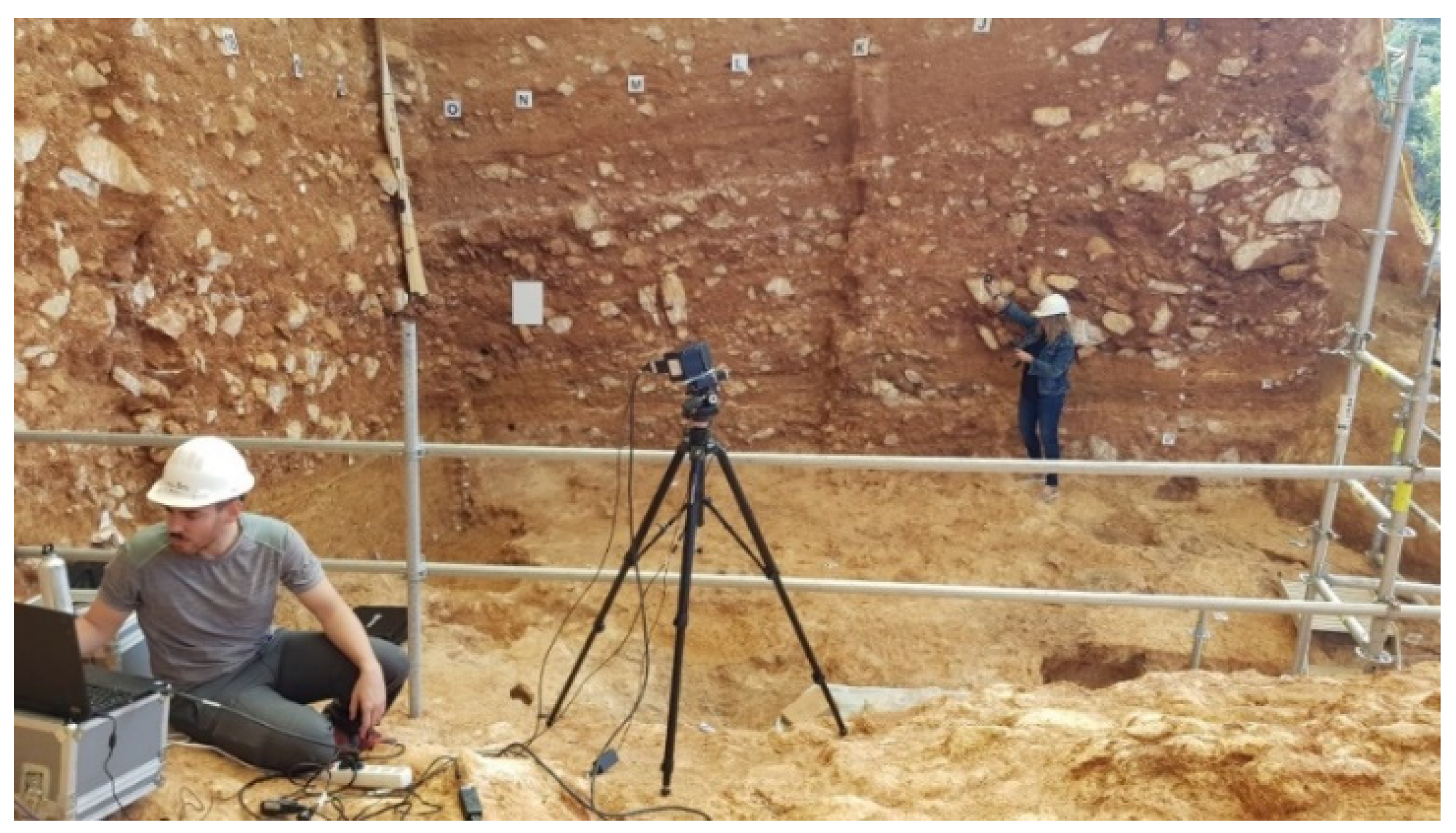
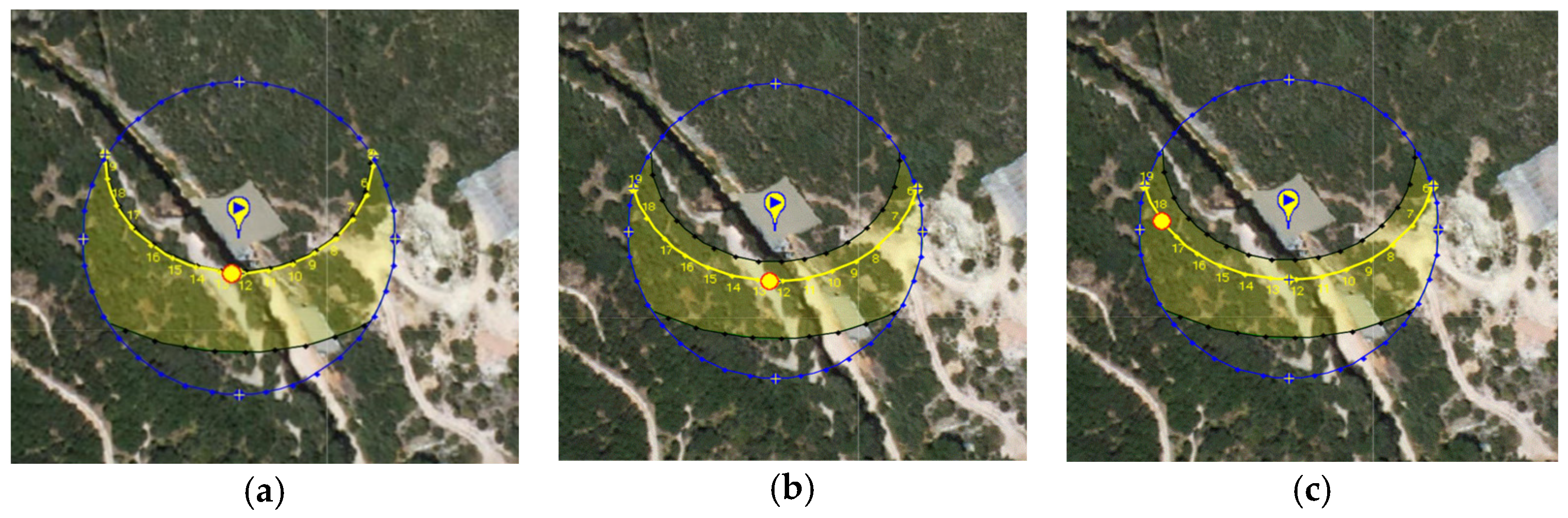
3.1. Experimental Measures and Image Acquisition

Hyperspectral imaging (HSI) was carried out on the exposed upper surface of the Gran Dolina site, focusing on the southeastern portion of stratigraphic level TD10. The experimental setup for HSI measurements is illustrated in Figure 4. Measurements under both indirect and direct daylight conditions allowed comparative analysis of near- and far-field imaging.
A hyperspectral imaging system operating in the VIS-NIR range (380–1000 nm) was used to capture images of the stratigraphic deposits in reflectance mode. This system included a VNIR A-series hyperspectral camera (Headwall Photonics, Inc., Bolton, MA, USA) with 17 mm lens (Schneider Kreuznach Xenoplan 1.4/17-0903, Jos. Schneider Optische Werke GmbH, Bad Kreuznach, Germany) [33]. The camera used for the measurements was a 12-bit model with a recording rate of 17.5 frames per second. The system operates using line scanning, facilitated by a computer-controlled turntable platform, with data acquisition and control managed through Hyperspec III v3.1.5 software (Headwall Photonics, Inc., Bolton, MA, USA). During a complete rotation (approximately 30 min), a series of images were captured using the HSI camera mounted on a tripod behind the starting point, precisely aligned with the sample’s center. The camera’s array detector resolution is 1004 × 810 pixels (spatial × spectral bands) with a spatial resolution of 7.4 μm per pixel and a total of 324 spectral bands.

Indirect and Direct Natural Lighting HSI Measurements

Two HSI datasets were acquired from the TD10 stratigraphy using indirect and direct natural lighting conditions. The first series, taken from a distance of 6 m, covered an area of 7.5 m in length by 3.5 m in width. The second series, from a closer distance of 2.7 m, captured an area measuring 3.2 m by 1 m.
Measurements were performed on-site on 3 June (Figure 5a) and 22 August (Figure 5b), 2022, under indirect sunlight, as well as on 22 August 2022, under direct sunlight conditions (Figure 5c) with partly cloudy skies and temperatures ranging from 20 °C to 28 °C. The solar path diagram is represented in Figure 5a–c, with a red marker indicating the azimuth and elevation of the sun based on the specific hour, day, and year of the measurements. These dates were selected not only to coincide with suitable solar orientation—ensuring the desired lighting conditions at the measurement area—but also to take advantage of stable and favorable weather forecasts (© 2009–2023 SunEarthTools.com, URL: https://www.sunearthtools.com (accessed on 1 May 2025)).

3.2. Data Processing: Endmember Extraction and Statistical Classification Methods

The high spectral resolution provided by hyperspectral imaging (HSI) allows for precise characterization of geoarchaeological classes at both spatial and spectral levels. However, the extensive detail in HSI data can result in large datasets, which require significant computational resources. To reduce dataset dimensions and enhance processing speed while maintaining accuracy, specific data processing techniques are implemented [34]. This section details the HSI processing methods used to detect reflectance changes, utilizing Matlab’s Image Processing Toolbox™ Hyperspectral Imaging Library. The primary steps in hyperspectral image analysis include (1) preprocessing (calibration and visualization), (2) processing (endmember detection), (3) postprocessing (endmember classification), and (4) exploration (results).

3.2.1. Preprocessing

To calibrate the hyperspectral data cube, we converted image data from raw digital counts to reflectance values (Rs), adjusting for illumination and sensor response [35]. The relative reflectance Rs is defined as
Rs = Is λ     Id \ \ \ ( λ \ \ \ ) Ir λ     Id \ \ \ ( λ \ \ \ ) × Rr ( λ )
where Is represents sample image data, Ir is the reference image (Spectralon® White Diffuse Reflectance Standard), Id is the dark current image taken without light, Rr is the reflectance factor (75%) of the white reference board, and λ is the wavelength in the electromagnetic spectrum.
Subsequently, a region of interest (ROI) was selected to focus on areas containing the most relevant data, eliminating non-precise regions. For indirect light measurements, the ROI matched the full image area, while under direct light, it was confined to red-boxed areas. The RGB image displays the main representative bands (R, G, and B channels), corresponding to photopic vision, covering wavelengths from 390 to 760 nm.

3.2.2. Signal Processing, Data Extraction, and Treatment

Spectral unmixing was performed to decompose mixed pixel data into constituent endmembers. This process involved two steps: (1) endmember extraction to identify dominant endmember signatures and (2) abundance mapping to estimate the proportion of each component in each pixel. The endmembers represent distinct and spectrally pure signatures that characterize the specific physical and chemical properties of individual surface materials. The number of endmembers was estimated using virtual dimensionality (VD), determined via the noise-whitened Harsanyi–Farrand–Chang (NWHFC) method [36], based on the Neyman–Pearson detection theory. To minimize data loss, the false alarm probability was adjusted to select the optimal number of endmembers.
Endmember signatures were determined using the N-Findr algorithm [37] and the maximum noise fraction (MNF) transformation. The MNF approach optimizes the signal-to-noise ratio in principal component bands rather than maximizing variance. This transformation is effective in isolating primary component bands that are spectrally distinct from noisier images. N-Findr is an efficient spectral feature extraction method, which operates by maximizing the N-dimensional volume formed by the purest pixels. Each pixel’s spectrum replaces an endmember candidate iteratively, recalculating the volume to retain the largest result. After spectral smoothing using Gaussian filtering to reduce noise, the first higher-order derivative endmember spectra were analyzed to distinguish spectrally similar materials [38]. The first derivative calculated the rate of change in reflectance over wavelengths.

3.2.3. Postprocessing, Data Modeling, and Image Classification

To assess the similarity between spectra and defined endmembers, we employed the spectral angle mapper (SAM) classification algorithm [39], a validated, automated approach suitable for geological mapping under natural lighting. SAM calculates the angle between spectral signatures, comparing each pixel vector in n-dimensional space to reference spectra based on geometric similarity. The most similar test spectrum is identified by the smallest angle or minimum distance; conversely, the least similar is identified by the largest angle.
Endmember abundance maps were generated using the fully constrained least squares (FCLS) method [40], which imposes both non-negativity and sum-to-one constraints on the linear unmixing model. Subsequently, maximum abundance classification (MAC) was applied to delineate spatial regions within the hyperspectral dataset based on the dominant endmember in each pixel. This approach facilitated a more detailed interpretation of the spatial distribution and dominant sedimentary features within the TD10 stratigraphic unit, as inferred from endmember classification.

4. Results of Hyperspectral Analysis Under Indirect and Direct Natural Lighting Conditions

This section presents the results of the hyperspectral analysis under indirect and direct natural lighting conditions, comparing the corresponding processing outcomes in each case. RGB image processing highlights the most representative bands of the red, green, and blue (R, G, and B) channels within the defined spectral range (see Figure 6a, Figure 7a and Figure 8a).
The endmember classifications presented in Figure 6b, Figure 7b and Figure 8b,d highlight the most prominent spectral responses of the sedimentary deposits and surface materials in the study area, as inferred from their reflectance characteristics. Environmental variables—including lighting conditions, the presence of roofing, shadowing effects, and surface moisture—can influence the radiance detected by the sensor, particularly under low signal intensity, thereby affecting measurement accuracy.
Additional factors such as material roughness, porosity, and the spatial resolution (pixel size) also play a critical role in the precision of endmember classification [40,41]. Furthermore, the spectral sensitivity of the sensor, especially at the boundaries of its wavelength detection range, significantly impacts the reflectance signal. Variability in solar irradiance and incident angle modulates the spectral profile, while the identification of reflectance minima is facilitated through the first derivative of the endmember spectra, where the derivative equals zero at wavelengths corresponding to local maxima (Figure 6c, Figure 7c and Figure 8c,e) [39].
The spectral profiles of each pixel in the reflectance image are compared to endmember signatures using the spectral angle mapper (SAM) classification. SAM calculates the spectral angle error to assess similarity between the spectral profiles, as shown in Figure 6 and Figure 7, where each pixel is represented by the endmember signature associated with its maximum abundance value. Unmixing abundance maps, used in hyperspectral classification, addresses spectral variability and indicates the proportion of each endmember within each pixel’s spectrum (see Figure 9, Figure 10 and Figure 11). Fractional abundance values are normalized along the color bar, ranging from blue (0, indicating absence) to red (1, indicating maximum presence).
Spectral classification enables a qualitative assessment of surface properties, including color variability, textural and morphological features, and the spatial distribution of materials, such as sediment size, homogeneity, and dispersion patterns. Table 3 and Table 4 summarize the predominant spectra, homogeneity, and location of sediment and material types derived from the endmember classification.

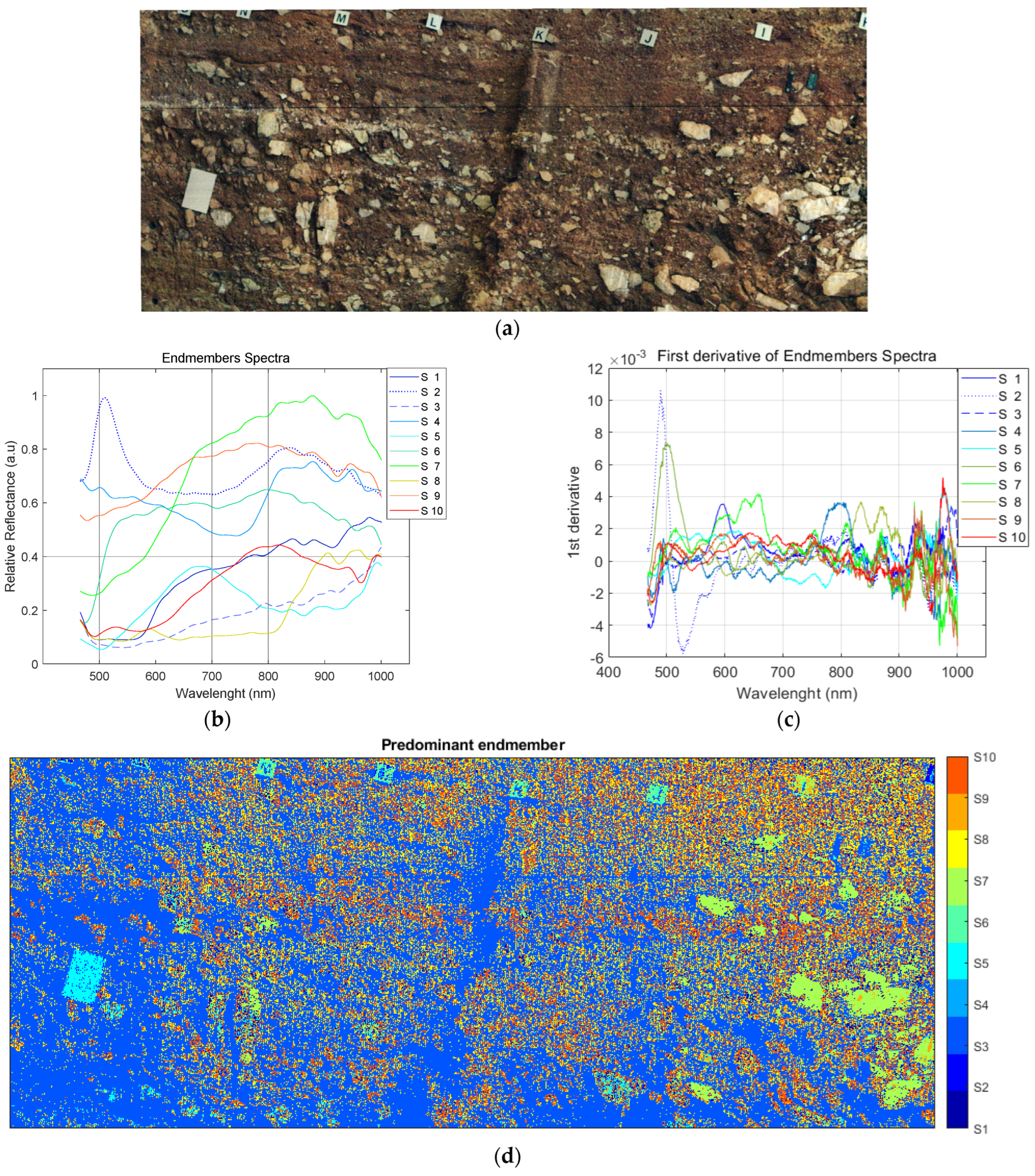
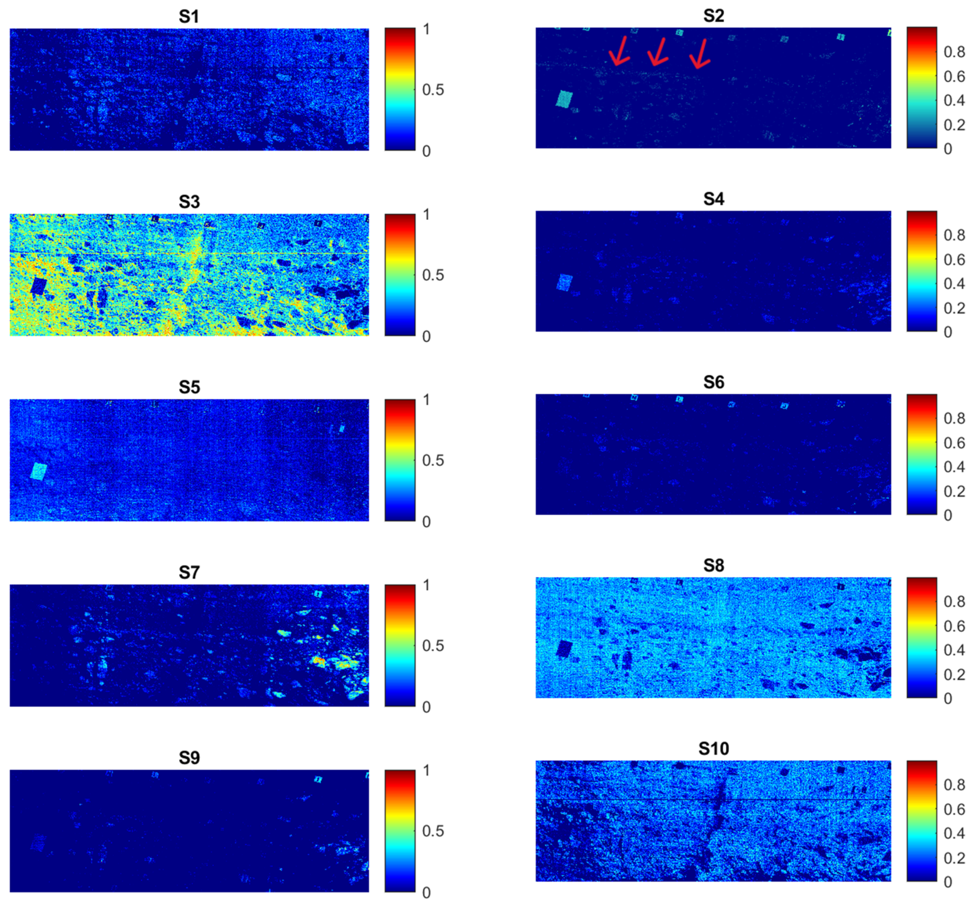
4.1. Experimental Measurement and Indirect Natural Lighting

This subsection presents results from hyperspectral imaging (HSI) measurements taken at both far and near distances under indirect light conditions (Figure 6a).
The spectral angle mapper (SAM) metric analysis revealed that the maximum similarity percentages were 50.26% for S5, 28.14% for S2, and 21.15% for S8. Minimum similarity values were 63.48% for S1, 32.53% for S7, 1.41% for S3, and 1.31% for S9. Figure 9 illustrates the spectral abundance map for each endmember, detailing the spatial distribution of their respective spectral signatures (Figure 6d).
The second column of Table 3 lists the predominant wavelength ranges where spectral peaks are observed, with each peak corresponding to the highest value for each endmember. The third column describes the distribution pattern in the abundance map, which strongly correlates with the surface morphology. Larger materials exhibit greater areas of concentrated abundance (S1, S3, and S7), whereas areas with smaller elements demonstrate higher spectral mixing, suggesting a more heterogeneous composition (Figure 6d). Notable materials include bones, represented by S2 (indicated by arrows) and S4 in the light blue horizontal lines. For regions studied, consistent spectral responses are observed, particularly for materials like mud. S8 and S7 show the near-infrared (NIR) response of mud, while S10 reflects an infrared (IR) response. Material degradation varies depending on vertical position and proximity to more exposed cave surfaces (e.g., S10 and S3). Moreover, façade orientation influences both the degree of weathering and surface moisture retention (S3). The fourth column lists the primary elements and objects linked to each endmember and their layer and location. The VIS-NIR reflectance spectrum of a limestone block typically shows a low to moderate reflectance in the visible range (380–700 nm), with a slight increase from the blue to red wavelengths due to its generally light coloration. In the NIR region (700–1000 nm), reflectance gradually increases, showing a smoother and more uniform spectral shape. The spectrum lacks sharp absorption features in this range, which is consistent with the mineralogical composition of limestone, primarily composed of calcite (CaCO3), a mineral that exhibits minimal absorption in the VIS-NIR region (S4 and S9).
The results obtained from near-field measurements are influenced by the spatial resolution of the imagery and the spectral mixing effects occurring within individual pixels. The near-HSI response and its processing under indirect lighting conditions are shown in Figure 7 and Figure 10. The highest SAM similarity is observed in Sn7 (91.89%), followed by Sn1 (6.56%) and S3 (1.55%), while the lowest similarity is found in Sn5 (53.90%), Sn6 (22.14%), Sn8 (21.02%), and Sn4 (2.55%) (Figure 7d). Figure 10 illustrates the quantity and spatial distribution of each endmember individually.
The endmembers identified in bone-bearing areas (Sn1, Sn3, and Sn5; see arrows in Figure 10) exhibit a mixed spectral response, combining signals from bones with those of surrounding stones and limestone. The concentration or dispersion of these endmembers is influenced by the surface’s roughness and morphometry. Varying levels of mud detection are observed in Sn2, Sn4, Sn6, and Sn8, while shadows are represented by Sn7 (Table 4).

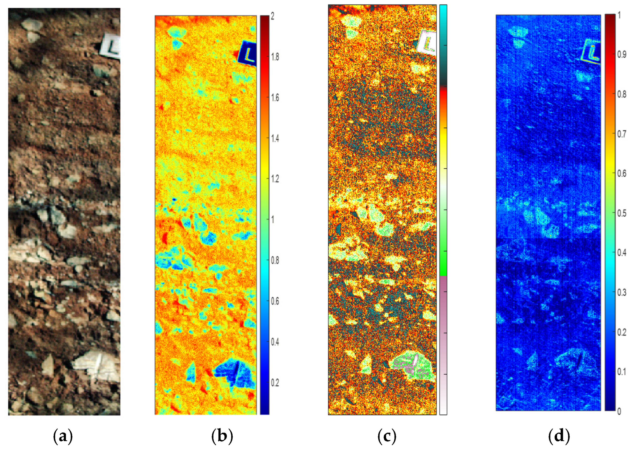
4.2. Experimental Measurement and Direct Natural Lighting

The analysis under direct natural lighting conditions was performed on two vertical HSI sections of the TD10 unit, labeled A and B (Figure 8a).
Higher spectral variations are observed in the spectral ranges of 400–500 nm and 850–1000 nm. Additionally, alterations caused by the signal from shadowed areas are detected in the upper left quadrant of Figure 8d. The abundance map of each endmember is shown in Figure 11, with crop A labeled as SCA and crop B labeled as SCB.
Figure 12 shows the RGB image of crop B (a). The sum of the abundance maps obtained from endmembers SCB4 (brown mud) and SCB10 (dark shadows) allows for the differentiation of the other components and their distribution. This map is presented in a standard color map (b) and a custom color map (c). The custom color map highlights discontinuities and changes in the different layers more distinctly. Two dark, inclined bands with high concentrations are observed, and the arrangement and orientation of the stones are also determined. The abundance map of SCB2 and SCB3 is shown in Figure 12d.

5. Discussion

The hyperspectral imaging (HSI) technique has emerged as a powerful analytical tool across various scientific disciplines, enabling the discrimination of distinct quality and spectral attributes. However, its application in the field of geoarchaeology, particularly within Paleolithic sites, has been limited due to specific challenges related to location and environmental conditions. This study presents a straightforward method for measuring and classifying geological and archaeological materials at historic sites, which can facilitate the precise management and characterization of cultural heritage information.
Traditionally, color differences caused by geological changes have been evaluated through visual perception. In contrast, HSI provides more objective data. Previous analyses of the southeast stratigraphic TD10 unit at Gran Dolina, based on the Munsell Soil Color Chart, identified three distinct color varieties within the photopic visual range (380–780 nm): yellowish red 5YR 5/8, reddish yellow 5YR 6/8, and reddish yellow 5YR 7/8, as detailed in Table 2.
This work assesses spectral reflectance differences through several predominant spectral endmembers that have been automatically identified. The proportion of each pixel containing these endmembers was calculated (see Figure 9, Figure 10 and Figure 11), allowing for accurate identification of the spectral concentration and distribution of elements and sediments. While visual evaluation can be influenced by factors such as the characteristics of the observer’s visual system and the illumination used, the HSI methodology provides a consistent statistical classification that enhances precision in identifying outcrop characteristics (e.g., stones and potential bone-like structures) and sediment types (e.g., mud and debris flow), even under varying lighting conditions. This approach enables the differentiation of similar elements that may appear identical or nearly so to the naked eye. Notably, spectral detection in the near-infrared (NIR) range is impossible to achieve without HSI; however, this technique captures spectral responses in the NIR range effectively.
The analysis and processing of HSI data enable the spectral characterization and spatial mapping of key surface components—such as specific lithologies, sediment types, or discrete objects—through endmember identification. Additionally, the use of spectral derivatives enhances classification and improves resolution, aiding in the identification and separation of individual spectral contributions. Results indicate that measurements obtained under direct illumination exhibit more stable values in the central part of the spectral range, while extreme ends show high slopes.
The resulting abundance maps reveal spectral and spatial discontinuities and accumulations that correspond to variations in material composition, such as changes in sediment types, the presence of concentrated lithic fragments, or localized deposits. Utilizing both local and global probabilities for mixed pixel characterization enables qualitative and quantitative evaluations. Results obtained from far-field measurements demonstrate a capacity to discriminate more uniform distributions, aligning well with prior field observations. Conversely, the spectral abundance map derived from close-distance measurements delineates a well-defined zone adjacent to the archaeological and paleoanthropological stratigraphic deposits. Moreover, independent processing of spectral reflectance for each endmember highlights differences, similarities, and material accumulations.
A subtle horizontal feature visible in the upper center of the image (Figure 9: S2; Figure 7: S1 and S3) is interpreted as corresponding to bone remains. Some spatial distributions associated with the blue spectral range (Figure 9: S1) and the NIR range (Figure 9: S8) are not clearly distinguishable in the RGB image, highlighting the added value of hyperspectral data for detecting subtle spectral variations. Several factors, including humidity and degradation from exposure to the elements (Figure 9: S3) or material displacement due to handling, contribute to blurring in the data.
The close-up images provide a clearer identification of areas (Sn5), except where stained by the surrounding matrix, which appears relatively uniform (mostly Sn7). Classes Sn1 and Sn3 exhibit a blue tendency associated with stones and bones (see Figure 7c). Direct natural lighting analysis facilitates the differentiation of smaller areas. Increased light intensity permits the evaluation of minor variations; however, the solar incidence angle can introduce shadows due to surface roughness, inclination, and infrastructural obstructions.
Variations in lighting conditions, image resolution, and spatial scale between far- and near-field measurements facilitate the characterization of diverse landscape mosaics, revealing dominant spectral patterns and material compositions. The hyperspectral analysis reveals significant spectral variations in the 400–500 nm and 850–1000 nm ranges, highlighting key differences in material composition. Shadow-induced alterations can significantly hinder the retrieval of spectral information, often obscuring key surface features and compromising signal interpretation.
The distribution of different materials is effectively mapped, allowing for a clearer differentiation of components. Additionally, the use of a custom color map enhances the visualization of layer discontinuities and structural patterns, such as the orientation of stones and the presence of high-concentration bands. Results from near-field measurements are influenced by image resolution and spectral mixing effects within individual pixels, which must be taken into account when interpreting detailed material distributions.
These findings are consistent with results obtained in other international geoarchaeological studies where HSI has been successfully applied for material characterization, stratigraphic mapping, or the identification of anthropogenic features in archaeological deposits. Studies such as those by Zhao et al. [42] in Chinese loess–paleosol sequences and by Bardelli et al. [43] in Mediterranean prehistoric contexts reinforce the potential of HSI to detect fine-scale compositional and spectral variations that traditional techniques may overlook. By integrating these insights, the present study contributes to the growing body of literature advocating for the broader implementation of hyperspectral methods in heritage science and geoarchaeological applications.

6. Conclusions

In summary, the experimental HSI measurement procedures conducted at Gran Dolina cave in Atapuerca (Sierra de Atapuerca, Burgos, Spain), coupled with subsequent data processing, have facilitated the hyperspectral characterization of diverse elements and materials from the TD10 sediment. This study outlines a comprehensive exploration method that includes experimental data collection, supervised statistical classification, and spectral derivative processes for both far- and near-field analyses.
Overall, the findings highlight the significant characteristics of stratigraphic information derived from endmember extraction techniques applied to hyperspectral data, in accordance with the statistical classification methods used to compare image spectra under varying illumination conditions. Data processing encompasses both global and local classifications within the predominant spectrum, including the NIR spectrum, which is undetectable by human vision or conventional cameras. This spectral classification enables spatial quantification and differentiation of significant responses.
The hyperspectral assessment of archaeological and paleoanthropological stratigraphic deposits serves as a potent digital resource, contributing to the sustainable management of cultural heritage information and enhancing environmental sciences. The hyperspectral imaging (HSI) assessment of archaeo-paleoanthropological stratigraphic deposits at Atapuerca, as presented in this study, underscores the increasing relevance of HSI in cultural heritage and paleoanthropological research.
The proposed methodology, which integrates HSI measurements with statistical classification techniques, aligns with the broader applications of hyperspectral imaging in the cultural heritage field. Furthermore, the Atapuerca study highlights the importance of spectral models for material classification, emphasizing the role of machine learning in the study of deposits within cultural heritage research. By leveraging HSI for the digital characterization of stratigraphic deposits, this research not only contributes to human evolution studies but also supports sustainable management practices, reinforcing the potential of HSI as a fundamental tool in both archaeological and heritage science.

Author Contributions

Conceptualization, B.G.-F. and A.B.-C.; data capture and methodology, B.G.-F., A.B.-C. and A.M.-F.; project administration, B.G.-F. and A.B.-C.; software, B.G.-F. and A.B.-C.; validation, B.G.-F., A.B.-C., A.M.-F. and I.C.; formal analysis, B.G.-F.; investigation, B.G.-F., A.B.-C., A.M.-F. and I.C.; resources, B.G.-F., A.B.-C., A.M.-F. and I.C.; writing—original draft preparation, B.G.-F. and I.C.; writing—review and editing, B.G.-F., A.B.-C., A.M.-F., I.C., A.O., P.S., M.M.-T. and M.M.; visualization, B.G.-F., A.B.-C., A.M.-F. and I.C.; supervision, A.O., P.S., M.M.-T. and M.M. All authors have read and agreed to the published version of the manuscript.

Funding

This research did not receive any specific external funding.

Data Availability Statement

The data presented in this study are available on request from the corresponding author.

Acknowledgments

The authors gratefully acknowledge the support of Universidad Politécnica de Madrid (UPM), Spain. This research was facilitated by the work of Berta García Fernández during a research stay at the Spanish National Research Center on Human Evolution (CENIEH) between June and August 2022. Hyperspectral imaging was carried out using a VNIR A-Series Headwall Photonics camera at the Laboratory of Digital Mapping and 3D Analysis, CENIEH. Fieldwork at Atapuerca is supported by the Junta de Castilla y León and Fundación Atapuerca. The authors also acknowledge the indirect support provided through research projects PID2021-122355NB-C33 and PID2021-122355NB-C32, funded by MCIN/AEI/10.13039/501100011033 and co-financed by the European Regional Development Fund (ERDF)—“A way of making Europe”. Additional institutional support was received from the AGAUR agency (2021SGR01239 Research Group) and Universitat Rovira i Virgili (2023PFR-URV-01239). We also thank the EIA and TD10 excavation teams for their collaboration.

Conflicts of Interest

The authors declare no conflicts of interest.

References

  1. Pavia, D.L.; Lampman, G.M.; Kriz, G.S.; Vyvyan, J.R. Introduction to Spectroscopy; Cengage Learning: Boston, MA, USA, 2014. [Google Scholar]
  2. Saha, D.; Manickavasagan, A. Machine learning techniques for analysis of hyperspectral images to determine quality of food products: A review. Curr. Res. Food Sci. 2021, 4, 28–44. [Google Scholar] [CrossRef]
  3. d’Oleire-Oltmanns, S.; Marzolff, I.; Peter, K.D.; Ries, J.B. Unmanned aerial vehicle (UAV) for monitoring soil erosion in Morocco. Remote Sens. 2012, 4, 3390–3416. [Google Scholar] [CrossRef]
  4. Miřijovský, J.; Langhammer, J. Multitemporal monitoring of the morphodynamics of a mid-mountain stream using UAS photogrammetry. Remote Sens. 2015, 7, 8586–8609. [Google Scholar] [CrossRef]
  5. Gomez, C.; Purdie, H. UAV-based Photogrammetry and Geocomputing for Hazards and Disaster Risk Monitoring–A Review. Geoenvironmental Disasters 2016, 3, 23. [Google Scholar] [CrossRef]
  6. Adão, T.; Hruška, J.; Pádua, L.; Bessa, J.; Peres, E.; Morais, R.; Sousa, J.J. Hyperspectral imaging: A review on UAV-based sensors, data processing and applications for agriculture and forestry. Remote Sens. 2017, 9, 1110. [Google Scholar] [CrossRef]
  7. Asner, G.P.; Wessman, C.A.; Bateson, C.A.; Privette, J.L. Impact of tissue, canopy, and landscape factors on the hyperspectral reflectance variability of arid ecosystems. Remote Sens. Environ. 2000, 74, 69–84. [Google Scholar] [CrossRef]
  8. Transon, J.; d’Andrimont, R.; Maugnard, A.; Defourny, P. Survey of hyperspectral earth observation applications from space in the sentinel-2 context. Remote Sens. 2018, 10, 157. [Google Scholar] [CrossRef]
  9. Urbanos, G.; Martín, A.; Vázquez, G.; Villanueva, M.; Villa, M.; Jimenez-Roldan, L.; Sanz, C. Supervised Machine Learning Methods and Hyperspectral Imaging Techniques Jointly Applied for Brain Cancer Classification. Sensors 2021, 21, 3827. [Google Scholar] [CrossRef]
  10. Fischer, C.; Kakoulli, I. Multispectral and hyperspectral imaging technologies in conservation: Current research and potential applications. Stud. Conserv. 2006, 51 (Suppl. S1), 3–16. [Google Scholar] [CrossRef]
  11. Picollo, M.; Cucci, C.; Casini, A.; Stefani, L. Hyper-spectral imaging technique in the cultural heritage field: New possible scenarios. Sensors 2020, 20, 2843. [Google Scholar] [CrossRef]
  12. Jacq, K.; Debret, M.; Fanget, B.; Coquin, D.; Sabatier, P.; Pignol, C.; Arnaud, F.; Perrette, Y. Theoretical Principles and Perspectives of Hyperspectral Imaging Applied to Sediment Core Analysis. Quaternary 2022, 5, 28. [Google Scholar] [CrossRef]
  13. Linderholm, J.; Geladi, P.; Gorretta, N.; Bendoula, R.; Gobrecht, A. Near infrared and hyperspectral studies of archaeological stratigraphy and statistical considerations. Geoarchaeology 2019, 34, 311–321. [Google Scholar] [CrossRef]
  14. Doneus, M.; Verhoeven, G.; Atzberger, C.; Wess, M.; Ruš, M. New ways to extract archaeological information from hyperspectral pixels. J. Archaeol. Sci. 2014, 52, 84–96. [Google Scholar] [CrossRef]
  15. Guanter, L.; Richter, R.; Moreno, J. Spectral calibration of hyperspectral imagery using atmospheric absorption features. Appl. Opt. 2006, 45, 2360–2370. [Google Scholar] [CrossRef]
  16. Peyghambari, S.; Zhang, Y. Hyperspectral remote sensing in lithological mapping, mineral exploration, and environmental geology: An updated review. J. Appl. Remote Sens. 2021, 15, 031501. [Google Scholar] [CrossRef]
  17. Ortega, A.I.; Benito-Calvo, A.; Pérez-González, A.; Martín Merino, M.A.; Pérez-Martínez, R.; Parés, J.M.; Aramburu, A.; Arsuaga, J.L.; Bermúdez de Castro, J.M.; Carbonell, E. Evolution of multilevel caves in the Sierra de Atapuerca (Burgos, Spain) and its relation to human occupation. Geomorphology 2013, 196, 122–137. [Google Scholar] [CrossRef]
  18. Ortega, A.I.; Benito-Calvo, A.; Martín, M.A.; Pérez-González, A.; Parés, J.M.; Bermúdez de Castro, J.M.; Arsuaga, J.L.; Carbonell, E. Las cuevas de la Sierra de Atapuerca y el uso del paisaje kárstico durante el Pleistoceno (Burgos, España). Boletín Geológico Y Min. 2018, 129, 083–106. [Google Scholar] [CrossRef]
  19. Benito-Calvo, A.; Pérez González, A. Geomorphology of the Sierra de Atapuerca and the Middle Arlanzón Valley (Burgos, Spain). J. Maps 2015, 11, 535–544. [Google Scholar] [CrossRef]
  20. Benito-Calvo, A.; Ortega, A.I.; Navazo, M.; Moreno, D.; Pérez-Gonzalez, A.; Parés, J.M.; Bermúdez De Castro, J.M.; Carbonell, E. Pleistocene geodynamic evolution of the Arlanzón valley: Implications for the formation of the endokarst system and the open air archaeological sites of the Sierra de Atapuerca (Burgos, España). Boletín Geológico Y Min. 2018, 129, 059–082. [Google Scholar] [CrossRef]
  21. Martínez-Fernández, A.; Benito-Calvo, A.; Campaña, I.; Ortega, A.I.; Karampaglidis, T.; de Castro, J.M.B.; Carbonell, E. 3D monitoring of Paleolithic archaeological excavations using terrestrial laser scanner systems (Sierra de Atapuerca, Railway Trench sites, Burgos, N Spain). Digit. Appl. Archaeol. Cult. Herit. 2020, 19, e00156. [Google Scholar] [CrossRef]
  22. Campaña, I.; Benito-Calvo, A.; Pérez-González, A.; Ortega, A.I.; Bermúdez De Castro, J.M.; Carbonell, E. Using 3D models to analyse stratigraphic and sedimentological contexts in archaeo-palaeo-anthropological Pleistocene sites (Gran Dolina site, Sierra de Atapuerca). In CAA 2015 Keep the Revolution Going, Proceedings of the 43rd Annual Conference on Computer Applications and Quantitative Methods in Archaeology; Campana, S., Scopigno, R., Carpentiero, G., Cirillo, M., Eds.; Archeopress: Oxford, UK, 2016; pp. 337–345. [Google Scholar]
  23. Campaña, I.; Benito-Calvo, A.; Pérez-González, A.; Ortega, A.I.; Bermúdez de Castro, J.M.; Carbonell, E. Pleistocene sedimentary facies of the Gran Dolina archaeo-paleoanthropological site (Sierra de Atapuerca, Burgos, Spain). Quat. Int. 2017, 433, 68–84. [Google Scholar] [CrossRef]
  24. Campaña, I. Estratigrafía y Sedimentología del Yacimiento de Gran Dolina (Sierra de Atapuerca, Burgos). Ph.D. Thesis, University of Burgos, Burgos, Spain, 2018. [Google Scholar] [CrossRef]
  25. Bermúdez de Castro, J.M.; Arsuaga, J.L.; Carbonell, E.; Rosas, A.; Martínez, I.; Mosquera, M. A Hominid from the lower Pleistocene of Atapuerta, Spain: Possible ancestor to Neandertals and modern humans. Science 1997, 276, 1392–1395. [Google Scholar] [CrossRef] [PubMed]
  26. Carbonell, E.; Bermúdez de Castro, J.M.; Parés, J.M.; Pérez-González, A.; Cuenca-Bescos, G.; Ollé, A.; Mosquera, M.; Huguet, R.; van der Made, J.; Rosas, A.; et al. The first hominin of Europe. Nature 2008, 452, 465–469. [Google Scholar] [CrossRef] [PubMed]
  27. Ollé, A.; Mosquera, M.; Rodríguez, X.P.; de Lombera-Hermida, A.; García-Antón, M.D.; García-Medano, P.; Peña, L.; Menéndez, L.; Navazo, M.; Terradillos, M.; et al. The Early and Middle Pleistocene technological record from Sierra de Atapuerca (Burgos, Spain). Quat. Int. 2013, 295, 138–167. [Google Scholar] [CrossRef]
  28. Rodríguez, J.; Burjachs, F.; Cuenca-Bescós, G.; García, N.; Van der Made, J.; Pérez González, A.; Blain, H.-A.; Expósito, I.; López-García, J.M.; García Antón, M.; et al. One million years of cultural evolution in a stable environment at Atapuerca (Burgos, Spain). Quat. Sci. Rev. 2011, 30, 1396–1412. [Google Scholar] [CrossRef]
  29. Benito-Calvo, A.; Ortega, A.I.; Pérez-González, A.; Campaña, I.; Bermúdez de Castro, J.M.; Carbonell, E. Palaeogeographical reconstruction of the Sierra de Atapuerca Pleistocene sites (Burgos, Spain). Quat. Int. 2017, 433, 379–392. [Google Scholar] [CrossRef]
  30. Moreno, D.; Falguères, C.; Pérez-González, A.; Duval, M.; Voinchet, P.; Benito-Calvo, A.; Ortega, A.I.; Bahain, J.J.; Sala, R.; Carbonell, E.; et al. ESR chronology of alluvial deposits in the Arlanzón valley (Atapuerca, Spain): Contemporaneity with Atapuerca Gran Dolina site. Quat. Geochronol. 2012, 10, 418–423. [Google Scholar] [CrossRef]
  31. Parés, J.M.; Arnold, L.; Duval, M.; Demuro, M.; Pérez-González, A.; Bermúdez de Castro, J.M.; Carbonell, E.; Arsuaga, J.L. Reassessing the age of Atapuerca-TD6 (Spain): New paleomagnetic results. J. Archaeol. Sci. 2013, 40, 4586–4595. [Google Scholar] [CrossRef]
  32. Moreno, D.; Falguères, C.; Pérez-González, A.; Voinchet, P.; Ghaleb, B.; Despriée, J.; Bahain, J.-J.; Sala, R.; Carbonell, E.; Bermúdez de Castro, J.M.; et al. New radiometric dates on the lowest stratigraphical section (TD1 to TD6) of Gran Dolina site (Atapuerca, Spain). Quat. Geochronol. 2015, 30, 535–540. [Google Scholar] [CrossRef]
  33. Headwall Photonics Inc. Hyperspectral Imaging Sensors: Hyperspec VNIR. Available online: https://www.headwallphotonics.com/products/vnir-400-1000nm (accessed on 10 May 2025).
  34. Kale, K.V.; Solankar, M.M.; Nalawade, D.B.; Dhumal, R.K.; Gite, H.R. A research review on hyperspectral data processing and analysis algorithms. Proceedings of the national academy of sciences. India Sect. A Phys. Sci. 2017, 87, 541–555. [Google Scholar] [CrossRef]
  35. Polder, G.; van der Heijden, G.W.; Keizer, L.P.; Young, I.T. Calibration and characterisation of imaging spectrographs. J. Near Infrared Spectrosc. 2003, 11, 193–210. [Google Scholar] [CrossRef]
  36. Chang, C.I.; Du, Q. Estimation of number of spectrally distinct signal sources in hyperspectral imagery. IEEE Trans. Geosci. Remote Sens. 2004, 42, 608–619. [Google Scholar] [CrossRef]
  37. Winter, M.E. N-FINDR: An algorithm for fast autonomous spectral end-member determination in hyperspectral data. In Proceedings of the SPIE 3753, Imaging Spectrometry V, Denver, CO, USA, 19–21 July 1999. [Google Scholar] [CrossRef]
  38. Debba, P.; Carranza, E.J.; van der Meer, F.D.; Stein, A. Abundance estimation of spectrally similar minerals by using derivative spectra in simulated annealing. IEEE Trans. Geosci. Remote Sens. 2006, 44, 3649–3658. [Google Scholar] [CrossRef]
  39. Kruse, F.A.; Lefkoff, A.B.; Boardman, J.W.; Heidebrecht, K.B.; Shapiro, A.T.; Barloon, P.J.; Goetz, A.F.H. The Spectral Image Processing System (SIPS) Interactive Visualization and Analysis of Imaging Spectrometer Data. Remote Sens. Environ. 1993, 44, 145–163. [Google Scholar] [CrossRef]
  40. Kay, S.M. Fundamentals of Statistical Signal Processing: Estimation Theory; Prentice-Hall, Inc.: Hoboken, NJ, USA, 1993. [Google Scholar]
  41. Somers, B.; Asner, G.P.; Tits, L.; Coppin, P. Endmember variability in spectral mixture analysis: A review. Remote Sens. Environ. 2011, 115, 1603–1616. [Google Scholar] [CrossRef]
  42. Zhao, Y.; Liu, B.; Wang, X.; Xu, X.; Zhang, H. Hyperspectral analysis and classification of loess-paleosol sequences based on spectral indices and support vector machine. Int. J. Appl. Earth Obs. Geoinf. 2019, 79, 111–123. [Google Scholar] [CrossRef]
  43. Bardelli, L.; Cattaneo, C.; Colombo, A.; Ricci, M.; Zerbi, C.M. Hyperspectral imaging applied to cultural heritage: Classification and mapping of pigment traces in prehistoric rock art. Spectrochim. Acta Part A Mol. Biomol. Spectrosc. 2020, 229, 117998. [Google Scholar] [CrossRef]
Figure 1. Satellite view of the Atapuerca sites (Sierra de Atapuerca, Burgos, Spain), showing the location of Gran Dolina cave (red number 1).
Heritage 08 00233 g001
Figure 2. Sedimentary facies of Gran Dolina southeast stratigraphic TD10 level [23].
Heritage 08 00233 g002
Figure 3. (a) Measurement area location of experimental setup carried out in Gran Dolina cave on Atapuerca (Sierra de Atapuerca). The yellow box highlights the stratigraphic interval studied in this work, which includes units 10.4 to 10.1. (b) Sedimentary facies described in TD10. Black lines indicate stratigraphic limits [24].
Heritage 08 00233 g003
Figure 4. The Gran Dolina cave at Atapuerca (Sierra de Atapuerca, Burgos, Spain)—experimental setup.
Heritage 08 00233 g004
Figure 5. Satellite view of Atapuerca sites (Sierra de Atapuerca, Burgos, Spain): Gran Dolina cave. Sun path diagram of the site: (a) 3 June (12:30 h) and (b) 22 August (12:30 h). (c) Sun path diagram of the site on 22 August 2022 (15:30 h). The yellow shaded area represents the overall solar trajectory at the site, while the yellow line indicates the solar path on the day of measurement. The red dot marks the position of the sun at the time of the experimental measurement, helping to assess sunlight exposure and potential shading conditions at the site.
Heritage 08 00233 g005
Figure 6. HSI measurements from a distance. (a) RGB image showing detail of the TD10 unit. (b) Spectral reflectance signature determined by each endmember. (c) First derivative of the spectral reflectance for each endmember. (d) Predominant endmember distribution.
Heritage 08 00233 g006
Figure 7. HSI measurements (near). (a) RGB image of the selected study area within the stratigraphic section of the TD10 unit. (b) Spectral signature of each endmember. (c) First derivative of the endmember spectral reflectance. (d) Predominant endmember distribution.
Heritage 08 00233 g007
Figure 8. HSI image crop of the stratigraphic section of the TD10 unit, captured under direct natural lighting conditions. (a) RGB image. (b) Spectral signature of each endmember in section A. (c) First derivative of the endmember spectral reflectance in section A. (d) Spectral signature of each endmember in section B. (e) First derivative of the endmember spectral reflectance in section B.
Heritage 08 00233 g008
Figure 9. Spectral abundance map for each endmember (far measurement). Bones indicated by arrows.
Heritage 08 00233 g009
Figure 10. Spectral abundance maps of each endmember in the near region). Bones indicated by arrows.
Heritage 08 00233 g010
Figure 11. Spectral abundance map of each endmember in the HSI image SCA and SCB (crop (a,b)), captured under direct natural lighting conditions.
Heritage 08 00233 g011aHeritage 08 00233 g011b
Figure 12. (a) The RGB image of B, (b) SCB4 plus SCB10 (standard color map), (c) SCB4 plus SCB10 (custom color map), and (d) SCB2 plus SCB3.
Heritage 08 00233 g012
Table 1. Brief description of the sedimentary facies of TD10 [22].
FaciesBrief Description
Debris flow CClast-supported boulders with muddy matrix
Debris flow DMatrix-supported boulders and gravels with muddy matrix
Debris flow FGrain-supported boulders
ChannelGrain-size decreasing gravels
FloodplainSilts and clays
DecantationClayey silts
Table 2. Sedimentary facies of TD10 according to the Munsell soil color chart.
SubunitLayerThick (cm)FaciesColor
TD10.1118ChannelYellowish red 5YR 5/8
225Debris flow FReddish yellow 5YR 6/8
320Debris flow FReddish yellow 5YR 6/8
415ChannelReddish yellow 5YR 6/8
530Debris flow DYellowish red 5YR 5/8
625DecantationYellowish red 5YR 5/6
725Debris flow FReddish yellow 5YR 6/8
TD10.2115Channel/decantationReddish yellow 5YR 6/8
245Debris flow FReddish yellow 5YR 6/8
335Debris flow CYellowish red 5YR 5/8
420Debris flow FReddish yellow 5YR 6/8
530Debris flow FReddish yellow 5YR 6/8
650Debris flow CStrong brown 7.5YR 5/6
TD10.3135Debris flow FReddish yellow 5YR 6/8
245Debris flow FReddish yellow 5YR 6/8
TD10.4130Channel/floodplain/decantationYellowish red 5YR 5/8
Table 3. Sedimentary characteristics of TD10 based on endmember classification (far region).
Main LocationSediment/ObjectSurface MorphologyPredominant Spectrum
(Spectral Peak)
Endmember
TD10 higher inMudUniform, irregular,
decreasing,
Orange-red + IR
(Peak 950 nm)
S1
upper right
TD10 middle and bottomBones,
Small stones,
gravels,
reference targets
ScatteredBluish-red + IR
(Peak 510 nm)
S2
TD10, higher in lower left and central vertical lineMudUniform, increasingReddish-brown
(Peak 1000 nm)
S3
TD10 centralBones and limestoneScatteredBluish-white–NIR
(Peak 950 nm)
S4
TD10 in left, upper and lower zonesReference targets,
stones
Uniform, irregular,
increasing
White-red
(Peak 880 nm)
S5
TD10Reference targetScatteredWhite
(Peak 800 nm)
S6
TD10, higher in leftStonesScatteredWhite-reddish
(Peak 880 nm)
S7
TD10MudUniform, irregularNIR
(Peak 900 nm)
S8
TD10 right leftLimestoneScatteredWhite
(Peak 780 nm)
S9
Entire, higher in upper right cornerMudUniform, irregular,
decreasing
Red–NIR
(Peak 800 nm)
S10
Table 4. Sedimentary characteristics of TD10 based on endmember classification (near region).
Main LocationSediment/ObjectSurface MorphologyPredominant SpectrumEndmember
(Spectral Peak)
TD10.1, upper right areaBones, stonesScatteredWhite-bluish +NIR
(Peak 1000 nm)
Sn1
TD10.1LimestoneScatteredReddish-brown
(Peak 720 nm)
Sn2
TD10.1Bones
and limestone
ScatteredWhite + NIR
(Peak 690 nm)
Sn3
TD10.1LimestoneScatteredBluish-white
(980 nm)
Sn4
TD10.1Bones, stonesScatteredWhite peak in red
(680 nm)
Sn5
TD10.1MudUniformBrown-reddish–NIR
(Peak 990 nm)
Sn6
TD10.1MudScatteredBrown-reddish–NIR
(Peak 1000 nm)
Sn7
TD10.1MudIrregular, uniformBrown-reddish–NIR
(Peak 1000 nm)
Sn8
Disclaimer/Publisher’s Note: The statements, opinions and data contained in all publications are solely those of the individual author(s) and contributor(s) and not of MDPI and/or the editor(s). MDPI and/or the editor(s) disclaim responsibility for any injury to people or property resulting from any ideas, methods, instructions or products referred to in the content.

