Abstract
Edge detection is essential for numerous applications in various engineering and scientific fields, including photogrammetry and computer vision. Edge detection can be applied to a variety of 2D and 3D data types, enabling tasks like feature extraction, object recognition and scene reconstruction. Currently, 2D edge detection in image data can achieve high accuracy through various automated methods. At the same time, edge detection in 3D space remains a challenge due to the computational demands and parameterization of existing algorithms. However, with the growing volume of data, the need for automated edge extraction that delivers high accuracy and reliable performance across diverse datasets has become more critical than ever. In this context, we propose an algorithm that implements a direct method for automated 3D edge detection in point clouds. The suggested method significantly aids architects by automating the extraction of 3D vectors, a process that is traditionally time-consuming and labor-intensive when performed manually. The proposed algorithm performs edge detection through a five-stage pipeline. More specifically, it utilizes the differences in the direction of normal vectors to identify finite edges. These edges are afterwards refined and grouped into segments which are then fitted to highlight the presence of 3D edges. The proposed approach was tested on both simulated and real-world data with promising results in terms of accuracy. For the synthetic data, the proposed method managed to detect 92% of the straight edges for the higher density meshes.
1. Introduction
Edge detection is a well-investigated topic in the areas of photogrammetry and computer vision with applications spanning numerous domains, focusing on both two-dimensional (2D) and three-dimensional (3D) data. Two-dimensional edge detection in image data has been studied for several decades, with a wide range of algorithms capable of delivering accurate results with minimal computational overhead and processing time. More specifically, line features can be extracted from images using various approaches, either exploiting classical pipelines, or the recently emerged methods on deep neural networks [1,2].
Regarding 3D edge detection, research has intensified in the last decade. The rapid advancements in artificial intelligence, robotics, and computer vision have amplified the need for accurate 3D edge detection techniques. Today, several automated and semi-automated methods exist for 3D edge detection. The exploitation of neural networks into 3D edge detection workflows [3] has led to the development of noise-resistant algorithms that produce reliable results. However, these algorithms often have high computational costs, and their training process is time-consuming. Additionally, many existing methods for 3D edge detection involve high levels of parameterization [4] or are still sensitive to noisy data [5]. Therefore, ongoing research focuses on developing even more reliable algorithms for extracting 3D edges which work universally across various datasets without requiring minimal parameter adjustments and are resilient to data noise.
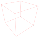
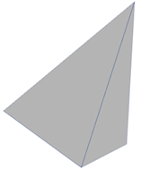
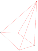
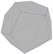
This paper proposes a direct automated method for detecting 3D straight edges in unorganized point clouds. The core idea of this method is to exploit the inclination differences in the normal vectors belonging to adjacent planes to identify the edges. This method utilizes a five-stage pipeline which begins with the generation of a mesh surface. Then, the finite edges of the mesh with a likelihood of forming the final straight 3D lines are grouped together based on the edge they belong to, concatenated into line segments and finally expanded to form the 3D edges. The algorithm is evaluated using both real-world and synthetic data in order to analyze its performance across different data and situations. The proposed method provides satisfactory results for data with and without noise, while the set parameter values can be used across different datasets without the need for any modifications. Figure 1 illustrates the basic steps of the algorithm developed.

Figure 1.
The basic steps of the methodology presented in this paper (more details in Section 3).
2. Related Work
To expedite the delineation of 3D line features in 3D models, 3D dense point clouds or to model surface discontinuities numerous edge detection algorithms have been proposed so far. For instance, ref. [6] models surface discontinuities based on matching edge features in 2D images and thus 3D lines, especially using large patch sizes. Specifically, ref. [6] improved the least squares matching approach using the edge information. Meanwhile, the 2D or 3D architectural drawings are still created manually, using 2D photogrammetric products and a CAD environment, even for complex cultural heritage objects. Recently, machine learning algorithms have been tested for automated vectorization [7,8,9,10], aiming to reduce the time required, while maintaining the quality of an expert. Still, novel machine learning algorithms have not yet reached the level of maturity required to fully replace the established photogrammetric pipeline. As a result, 2D-3D vector drawings are often created manually by vectorizing 3D models and dense point clouds. However, the conventional photogrammetric pipeline for the creation of 2D and 3D vector drawings is a time consuming, labor-intensive process that requires the involvement of specialists from several scientific fields, e.g., surveyors and architects, during the entire process. In fact, the delineation of 3D lines can contribute to the automation of the creation of architectural vector drawings using novel machine learning algorithms or the conventional photogrammetric pipeline. Existing 3D edge detection approaches can be broadly categorized into two groups. The first category includes methods that detect edges in 2D space, typically using 2D images, and then project the extracted edges into the 3D space, often followed by a refinement process. The second category focuses on methods that extract edges directly in 3D space.
The methods of the first category notably benefit from the well-established body of 2D edge detection algorithms. In fact, 2D edge detection is a fundamental computer vision problem and thus various traditional edge detection operators can be exploited [11,12,13,14]. Furthermore, prominent handcrafted 2D line detectors like LSD [15], EDLines [16], and several extensions such as ELSED [17] are frequently exploited. While these traditional methods are computationally efficient, they often lack robustness especially in demanding imaging conditions. In recent years, advances in deep learning have led to the development of new 2D edge detection approaches that yield improved results [18,19,20]. Moreover, several methods extract the 3D-2D edges by grouping the pixels or points into groups with similar spectral or geometric characteristics [18,21,22]. The aforementioned methods omit the semantic meaning of each category as they consider only their spectral and geometric characteristics. In contrast, the edge detection methods belonging to second category leverage techniques such as model fitting, analytical geometry, semantically enriched images, etc., to achieve high-quality results. More concretely, the creation of 3D linear features like vectors, using the given 3D point clouds directly, can usually be conducted using either a manual or a semi-automatic process [23,24]. While these methods are commonly used, they are time consuming and extremely strenuous, highlighting the need to automate the vector extraction process using 3D point clouds [25].
To solve the previous problem, a 3D boundary extraction method [26] that detects facade objects in point clouds was proposed. This method localizes windows and doors using a set of predefined templates of these objects in combination with plane intersections. Furthermore, ref. [27] proposed an automated approach which first segments the 3D point clouds into planes and finally extracts the 3D edge points by applying plane intersection. Moreover, ref. [28] used the plane intersection by exploiting 2D edges defined on images in combination with their exterior orientation. Additionally, the 3D edges and planes can be extracted from point clouds using statistical approaches. For example, ref. [29] proposed a method which first calculates the covariance matrix of points’ neighborhoods and then decides if a point relies on a plane or on a sharp 3D edge by examining the eigenvalues and eigenvectors of the calculated covariance matrix. Furthermore, ref. [22] proposed a 3D edge detection approach which combines segmentation and 2D contour extraction techniques. More concretely, the 3D point cloud is first segmented into planes by applying a region growing and merging method. Then, the group of 3D points belonging to each plane is projected in 2D space to create a set of images. Afterwards, the 2D contours of each image are extracted using a conventional 2D contour detection algorithm. Finally, the detected 2D contours are projected back into 3D space to form the set of the detected 3D edges. A limitation of the aforementioned method is its inability to extract edges belonging to a curved object. Moreover, ref. [30] proposed a 3D edge detection method, which uses the relationships of analytical geometry as well as the properties of planes in combination with digital images. Specifically, the method exploits a set of edges detected on an image along with its exterior orientation to define the planes on which the edges lie. Inevitably, the 3D edge points belonging to each detected edge in the given point cloud also lie on that same plane and thus can be easily extracted. Beyond conventional RGB images, 2D edge detection operators can also be applied to 2.5D data such as range images. For instance, ref. [31] proposed an approach which applies the Canny operator [13] to range images to define a set of 2D edges. The detected 2D edges are then projected into 3D space resulting in the set of the detected 3D edges. Recently, ref. [32] proposed the 3DPLan algorithm. Specifically, the algorithm exploits the powerful SfM/MVS algorithms to detect 3D edges by feeding them with semantically enriched images. Thus, the sparse and dense 3D point clouds created using the 3DPlan pipeline includes a label for each point indicating whether a point constitutes an edge point or not. In fact, the detected 3D edge points should be decomposed into the points of each edge, which are then used in the vectorization process. Although the 3DPlan pipeline includes clustering algorithms to handle the aforementioned issue, their implementation should be improved. An algorithm that performs 3D edge detection on unorganized 3D point clouds by exploiting the direction differences in normal vectors that belong to adjacent surfaces was also introduced [33]. The results of this method are really promising; however, further optimizations are needed in order to improve the running time of the algorithm. Recent studies demonstrate that the 2D edge detection methods are more mature than the 3D edge detection ones, and they are characterized by high parametrization or require a large amount of labeled data [34]. Aggarwal et al., 2024 [34], proposed a learning-based approach which extracts 3D edges using depth images along with a four-stage pipeline. Apart from the amount of labeled data, their completeness is crucial for learning-based approaches [35]. Additionally, the 3D line segment extraction methods commonly rely on their 2D counterparts [35]. Xin et al., 2024 [35], proposed a two-stage pipeline which exploits a weighted centroid calculation along with geometric operators to extract high-quality 3D line segments using point clouds.
The previously referenced and briefly described methods for straight edge detection are summarized in Table 1 for a better overview. So far, all methods remain at the research level, and no method has been reported as universal or mature, as the problem is quite complicated. In addition, a comparison of the methods is not possible at this stage, because all methods used different datasets and input data to test their proof of concepts. Every research group used their own metrics for evaluation, and thus, no objective comparison, e.g., in terms of computer time or another metric, is possible.

Table 1.
Summarization of edge detection methods.
3. Methodology
The present contribution comprises a five-stage pipeline for extracting three-dimensional straight edges from point clouds, based on the direction differences in the normal vectors belonging to neighboring planes (Figure 1 and Figure 2). The code was entirely developed in a Python environment. The first stage involves the construction of a three-dimensional triangular surface (3D mesh) using the ball-pivoting algorithm [36]. In the second stage, the normal vector for each triangle of the mesh is calculated. The angle between the normal vectors of neighboring triangles sharing a common edge is then computed and assigned to the corresponding edge. In the third stage, graph theory is used to filter out the edges of the mesh that presumably do not belong to 3D straight edges. The remaining edges, referred to as finite edges, are then grouped to form the edge segments. In the fourth stage, the least squares method is applied to each group of finite edges to compute the optimal line segment representing the group. In the fifth and final stage of the algorithm, a variation of the RANSAC algorithm, proposed in this work, is used to extend the line segments to their maximum possible extent to create the final three-dimensional straight edge (final 3D edges) for each group of finite edges.
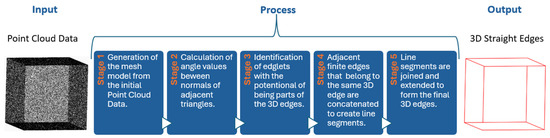
Figure 2.
Workflow of the proposed algorithm1.
3.1. Construction of the Triangle Mesh Surface
The construction of the triangular mesh from the points of the initial cloud is essential for creating the surface of the object described. In this context, the ball-pivoting algorithm [36] was chosen for surface reconstruction. This algorithm requires the selection of a sphere with radius ρ to traverse the cloud and create the mesh. The radius ρ of the sphere is user-defined, and multiple radii can be selected to fill any gaps which may occur in the triangular mesh during the algorithm’s execution. When using multiple radii, the algorithm operates sequentially, starting with the smallest radius and progressing to the largest. During the execution of the algorithm, special attention is required to both the choice of the sphere’s radius ρ and the density of the point cloud. For sparse point clouds, gaps may appear in the triangular mesh, if the radius of the sphere is not large enough to simultaneously contact neighboring points that are farther apart. However, simply increasing the radius is not an effective solution, as it can lead to overlooking important points and creating triangles with widely spaced points, which reduces surface details and introduces errors. According to the algorithm’s specifications, the point cloud density, provided there is no noise, should be such that the distance between neighboring points is less than half the length of the details that need to be captured. If this condition is met and the point cloud density is constant, selecting the radius of the sphere is relatively straightforward. However, in the case of non-uniform point cloud density, especially when combined with noise, the process becomes more complicated, requiring additional consideration to balance detail preservation and mesh accuracy.
In the present contribution, the density is calculated based on the distances between nearest neighboring points. However, in the case of irregular point clouds, there are areas where neighboring points are far apart and are not considered in the calculation of average density. Thus, it is inevitable that, in both cases, the clouds will have regions with lower point density than the calculated one and the final results will consequently have lower quality. To mitigate this problem, multiple radii were used in the ball-pivoting algorithm. More specifically, for every point cloud, a small radius equal to twice the average density of the cloud is first used to traverse the cloud. This initial small radius is used to capture all the details of the surface, but the created mesh inevitably contains many gaps. Then, a second, larger radius, equal to five times the average density of each cloud, is used to fill some of the gaps that are present in the triangular mesh created with the smaller radius. Even with this new radius value, some gaps in the triangular mesh remain. Increasing the radius further to fill these gaps is not advisable, as it introduces errors. For example, one common error would be the merging of very distant points that may not belong to the same plane, resulting in the creation of erroneous triangles. In conclusion, the ball-pivoting algorithm is performed automatically using two different radii, both to capture the details and to avoid gaps while minimizing the introduction of errors.
3.2. Computation of the Normal Vectors and Angle Estimation
The normal vector is computed for every triangle of the mesh, and the angle between the normal vectors of two adjacent triangles is subsequently calculated. This value, representing the inclination differences in adjacent planes, is then assigned to the shared edge of the two triangles. More specifically, a small angle between the two normal vectors implies that the planes containing these two triangles have an almost negligible angle between them, meaning they can be considered co-planar, and most probably their common edge does not belong to a straight edge. However, a large angle between the two normal vectors indicates a significant difference in the inclination between the planes containing the triangles. This suggests surface discontinuity and signals the presence of a straight edge segment, provided, of course, that the result is reliable and not caused by noise in the point cloud or any other error.
In order to correctly compute the angle between the normal vectors of neighboring triangles, special attention must be given to the direction of these vectors, as the direction of the normal vectors is initially arbitrary. However, it is necessary for the normal vectors of neighboring triangles to simultaneously point either inward or outward from the mesh. This alignment is crucial for correctly determining the angle that represents the slope difference between the planes of the neighboring triangles. The following method ensures that normal vectors are uniformly oriented, either inward or outward, across the mesh.
Let two triangles, ABC and XYZ, share a common side. First, it is ensured that vertices C and Z are the non-common vertices of the two triangles. Therefore, the side AB, or equivalently XZ, is the shared side of the two triangles (Figure 3). Next, the midpoint m of the segment CZ, which connects the non-common vertices of the two triangles, is calculated. Then, the vectors mb1 and mb2 are defined, pointing from the midpoint m of CZ to the centroids b1 and b2 of triangles ABC and XYZ, respectively. Finally, the dot product is calculated between the vectors mb1 and n1 (the normal vector corresponding to triangle ABC) and between mb2 and n2 (the normal vector corresponding to triangle XYZ).
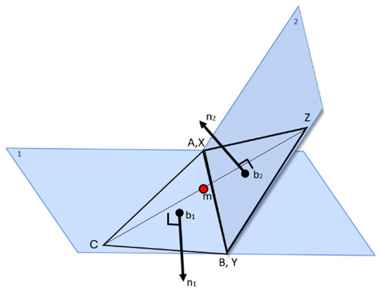
Figure 3.
Illustration of the process used to ensure that the normal vectors n1 and n2 which belong to adjacent triangles are consistently oriented to point inwards or outwards relative to the mesh.
It is well known that the dot product is positive for co-directional vectors and negative for oppositely directed vectors. Therefore, if the dot product between n1 and mb1 is negative, the vectors n1 and mb1 are oppositely directed. The same applies to vectors n2 and mb2. If the dot product between n1 and mb1 or between n2 and mb2 is negative, the corresponding vector is multiplied by −1 to reverse its direction. This ensures that the normal vectors n1 and n2 have the same direction as the vectors mb1 and mb2 and consistently point either inward or outward relative to the triangular mesh.
Once the desired orientation of the normal vectors is ensured, the angles between the normal vectors of adjacent triangles are computed and assigned to the shared edges of the triangles in the mesh. This process results in a 3D triangular network composed of points and edges. In this network, which will hereafter be referred to as the triangular mesh for brevity, the points store spatial information (coordinates) and the edges encode information about the inclination differences between the normal vectors of the triangles they correspond to.
3.3. Graph Generation
To simplify the data and thus improve the management of the relationships between the points of the 3D triangular mesh created in the previous stage, graph theory was employed. The use of graph theory not only simplifies the representation of the mesh but also facilitates solving the current problem using pre-existing algorithms. The triangular mesh, consisting of edges and points, was initially transformed into an undirected Cartesian graph G. The 3D points of the cloud with their Cartesian coordinates correspond to the nodes of the graph G, and the edges of the triangular mesh, which carry the information about the inclination difference between the normal vectors, correspond to the edges of G. During the creation of graph G, two threshold angles were also added to prevent some edges of the triangular mesh from becoming edges of the graph. In this way, the network is filtered, and the adjacencies between points that do not help in identifying the final 3D edges are not considered.
Regarding the thresholds chosen, the lower threshold is θ1 = rad and the upper threshold is θ2 = rad. Therefore, the values that are kept lie between the following inequality:
On one hand, the lower threshold θ1 is defined to ensure that the adjacent triangles, whose edges enter the graph, do not belong to the same plane, meaning that there is a significant angle between the planes containing them. On the other hand, the upper threshold θ2 is introduced to reduce errors caused by noise in the original point cloud. It is important to note that although the values of θ1 and θ2 have been chosen to fit a wide range of data, they can be modified by the user to better suit specific datasets, providing flexibility for varying data quality and characteristics.
In the next step of the algorithm, graph G is transformed into a line graph, L(G). During this process, the edges of G become nodes in the new graph L(G), and each edge of L(G) results from the connection of two vertices whose corresponding edges in G have a common vertex (Figure 4).
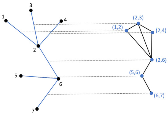
Figure 4.
Transformation of graph G to line graph L(G). The (blue) edges in the original graph G are converted into vertices (blue points) in the line graph L(G).
The purpose for this transformation is to group the edges of the original graph-and consequently the mesh- to map the different mesh edges to their corresponding final 3D edge. To obtain this grouping, it is necessary to know the relationships between neighboring edges in the mesh. However, since a graph inherently represents relationships between nodes rather than edges, the original graph G is transformed into line graph L(G). In this transformation, the edges of the first graph become the vertices of the second, enabling the representation of relationships between the edges of the original graph. This transformation makes it possible to efficiently analyze and group the mesh edges based on their connectivity and geometric properties.
In more detail, during the generation of line graph L(G), the angles formed by three consecutive points of graph G are calculated and a new angle threshold, θ = rad, is introduced. This threshold ensures that only adjacencies between the edges of G with angles greater than θ, and therefore, nearly collinear, are included in the adjacency list representing L(G). In this way, the edges of graph G can be grouped. The reason the chosen angle threshold is rad rather than the obvious π rad accounts for the inevitably noise in the initial point cloud data. Due to this noise, the edges of the triangles cannot be perfectly collinear. The angle tolerance of rad is used to prevent edges of the triangular mesh that are collinear and belong to the same final edge in the 3D space from being discarded.
3.4. Concatenation of Finite Edges
To find the optimal model which merges the grouped finite edges of the line graph L(G) into line segments, the least squares method (LSM) was employed. Specifically, for each group of edges resulting from the grouping process during the construction of the line graph, the goal is to identify the line segment the best fits the points corresponding to the endpoints of the edges within each group
The process begins by calculating the best-fitting line for the points that form the endpoints of the edges in each group using the LSM. Once the best-fitting line is established, all endpoint points are projected onto this line. From the projected points, the two with the greatest distance between them are identified. These points are then defined as the endpoints of the line segment being sought. This approach ensures a robust representation of the grouped edges while maintaining accuracy and minimizing error.
3.5. RANSAC Variation
The connection of the line segments that resulted from the implementation of the least squares method is performed using a variation of the random sample consensus (RANSAC) algorithm proposed in this paper. In this variation, a line segment is used as the original model and the goal is to extend it by connecting it with other line segments which meet certain conditions (inliers). These conditions require the line segment to be within a close distance of the model and form a maximum angle of θ = rad with it. The value of “close distance” is not fixed but is defined based on the given dataset.
To extend the initial model to identify the final edges, a depth-first search (DFS) algorithm was used. For the implementation of the proposed variation of RANSAC, a k-D tree was constructed to efficiently find the nearest neighbors in clouds of points with many elements. The use of the k-D tree significantly improves the performance of the algorithm by limiting the search for inliers to a predefined radius around the model, rather than examining the entire point cloud. This optimization drastically reduces the execution time of the algorithm, making it practical for processing large datasets containing millions of points within a reasonable computational timeframe.
The proposed variation differs from the original RANSAC for the following reasons:
- The original RANSAC is designed to randomly select point samples from the data and find the model, i.e., usually a line or plane, that best fits the inliers. In contrast, the proposed variation of RANSAC connects almost parallel line segments that are close to each other.
- The original RANSAC checks whether a point is an inlier based on a threshold related to the distance from the model. However, in the proposed variation, the line segments must form an angle smaller than rad with each other to be considered inliers. Additionally, their endpoints must be within a distance smaller than a predefined value. This distance is typically set to 5 times the average point density of the given point cloud but may be changed by the user if needed. The chosen distance provides a large enough area to search for neighboring line segments without introducing delays in the algorithm’s execution time.
- The original RANSAC does not use any special structure for searching for inliers, while in the proposed variation of RANSAC a k-D tree structure is employed to find the nearest neighbors. This approach narrows the search, restricting it to a smaller area so that the algorithm remains efficient even with datasets consisting of a large number of points. Some examples of the algorithm’s running times are available in Table 2. All experiments in this research were conducted on a PC equipped with an Intel i7 processor, 8GB of DDR4 RAM, and an NVIDIA GTX 1050 GPU.
Table 2. Differences in the algorithm’s running times due to the use of a k-D tree structure.
- The original RANSAC does not perform any searches for model extension based on neighboring points. However, in the proposed variation, an extension strategy is used by connecting neighboring line segments, which were found using the k-D tree structure. This extension is performed using depth-first search (DFS) algorithm, which joins the neighboring line segments that satisfy the distance and slope conditions of the model, thus forming the final edges.
4. Experimental Results
To evaluate the effectiveness and accuracy of the proposed algorithm, both real and synthetic datasets were used, with or without the presence of noise. On one hand, the use of real-world data helps to evaluate the performance of the algorithm in real conditions. On the other hand, synthetic data provide the ability to understand the behavior of the algorithm under given controlled conditions, making it possible to comprehend how various parameters, such as the noise level and cloud density, affect the produced results.
4.1. Synthetic Data
To test the algorithm, synthetic data with and without the presence of noise were used. This allowed for the evaluation of both the effectiveness of the proposed algorithm and the impact of noise on edge detection. All the synthetic data used were point clouds representing geometric shapes and were generated using Python code. For each shape, arbitrary noise was added to 10% of the points in the point cloud, with a standard deviation of 10% from the rest of the point cloud.
4.1.1. Noise-Free Synthetic Data
To extract the results from the above data, the algorithm was executed up to the stage of graph creation (stage 3). The subsequent two stages are only necessary if the data contains noise. As is clear from the detected edges depicted in Table 3, the algorithm poses no issues and is accurate when running on data without noise.
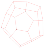
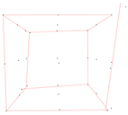
Table 3.
Representation of the triangular mesh and the 3D edges for the synthetic data without noise.
It is worth mentioning that for each of the previously discussed synthetic datasets, the result was obtained in less than one second. The correctness of these results is ensured, provided the triangular mesh is correctly created. This condition should always be verified before proceeding with the subsequent steps.
4.1.2. Noisy Synthetic Data
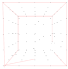
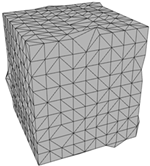
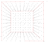
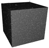
All the synthetic noisy point clouds used for the algorithm’s evaluation represent cubes with different densities. Table 4 illustrates the noisy synthetic data that were used in order to analyze how changes in point cloud density affect the algorithm’s performance. Specifically, the point clouds in Table 4 occupy the same volume, but each one contains a different number of points. For each of these point clouds, 10% of the points are noise, and the standard deviation of this noise is ±10%. These specific synthetic datasets were used to investigate the effect of point cloud density on the algorithm’s performance and the final edges.
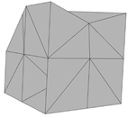
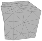
Table 4.
Representation of the triangular mesh and 3D edges for synthetic data with noise.
By analyzing the 3D edges detected in these point clouds, the influence of the data’s density on the accuracy of the algorithm’s results can be assessed. More specifically, it is evident from the examples depicted in Table 4 that a higher point cloud density leads to better results. More specifically, this can be validated by the last column of Table 4 which shows the percentage of correctly detected edges in accordance with increasing point cloud density. This occurs as sparse point clouds with noise often produce triangular meshes with gaps and errors, reducing the quality of subsequent algorithm steps and the accuracy of the final edges.
The examples in Table 4 illustrate that higher point cloud density minimizes errors in edge detection caused by poor quality of the triangular mesh. This observation was enabled by the fact that the synthetic data used represent normal shapes. However, determining the optimal density for accurate edge detection is challenging, as each point cloud varies in characteristics, like noise percentage, standard deviation, and inconsistent density.
4.2. Real-World Data
To evaluate the results of the proposed algorithm real-world data were also used. Below are the results for a dense point cloud of 3,093,022 points which represents the Temple of Demeter in Sangri, Naxos, Greece (Figure 5). This point cloud was derived from digital images collected in the field and, as expected, contains noise [37].
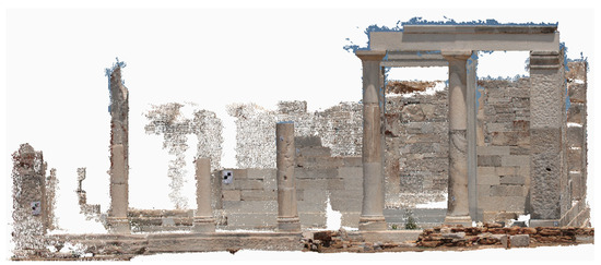
Figure 5.
Dense point cloud representing the temple of Demeter in Sangri, Naxos, Greece [37].
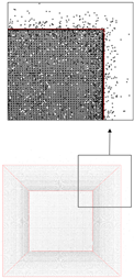
Figure 6 illustrates the triangular mesh of the dense point cloud, which was constructed using the ball-pivoting algorithm and, for the most part, forms a solid surface without gaps (Figure 6b). The level of density of a point cloud is undoubtedly directly related to its ability to describe the surface of the object with the required reliability while at the same time fulfilling the specifications of the scale of the final output. Thus, there is no general definition of point cloud density in terms of a number. The dense point cloud used in this experiment was the product of photogrammetric SfM/MVS processing digital images. However, in certain areas, such as where the capitals of the columns intersect with the architrave, several gaps are evident in the triangular mesh (Figure 6a). These gaps result from insufficient information in the specific regions of the images employed to generate the point cloud. Based on the above, it can be safely concluded that the density of the point cloud is not uniform. The non-uniformity of photogrammetric point clouds is caused by many factors, like inevitable occlusions, varying shadows, presence of texture, distance variations between the objects and the camera, etc.
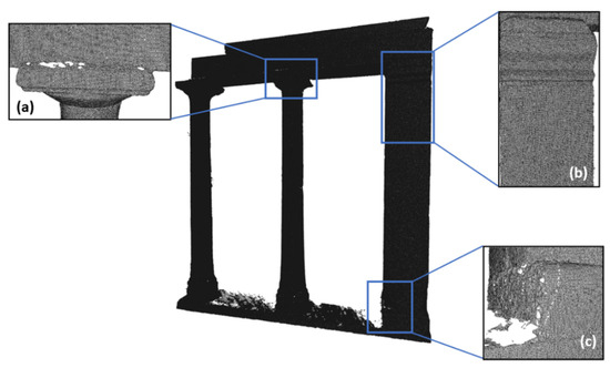
Figure 6.
Triangular mesh created from the dense point cloud of Demeter’s temple. (a) Area where gaps are formed in the mesh. (b) Area with a solid surface without gaps. (c) Area with gaps and other errors that create texture in the mesh.
This point cloud was the result of the implementation of automated SfM/MVS algorithms and consequently is considered unorganized. The characteristics of an unorganized point cloud such as this are as follows: (i) point density varies as it depends on image resolution, GSD (ground sampling distance), overlap, distance of features from the camera positions, and the reconstructed scene; (ii) points can directly inherit natural RGB colors from the captured images; and (iii) completeness depends on image overlap, with potential issues in areas lacking features or where shadows/textureless regions or occlusions exist. We embarked on a brief investigation into the uniformity and density of this point cloud, exploiting the pertinent functions of CloudCompare, a freeware software. In detail, both for the sparse and the dense point clouds, the number of points contained in a sphere of 1 m of diameter were determined. In Figure 7, the differentiation of the density of the sparse point cloud is presented in (a), and (b) shows the count diagram for the significant variations in the density. In Figure 8, the respective diagrams for the dense point cloud are presented. From both figures, it becomes evident that the point cloud using real data is not uniform, as its density varies considerably across the 3D space; thus, it is considered unordered, unorganized, and irregular.
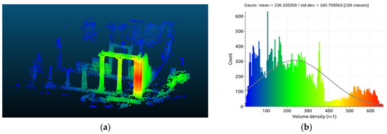
Figure 7.
The density (a) and distribution (b) of the real data sparse point cloud.
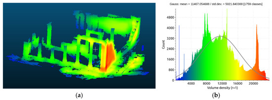
Figure 8.
The density (a) and distribution (b) of the real data dense point cloud.
In addition, some areas show significant inclination differences between neighboring triangles belonging to the same flat surface. This causes pronounced variations in the triangular mesh surface, for example, in the areas where the temple’s columns meet the stylobate (Figure 6c). Reasons for this phenomenon could be wear on the monument’s stones or the quality of the initial point cloud. These anomalies in the triangular mesh affect the final product of the 3D edge detection. Following mesh generation, the finite edges, which are parts of the final 3D edges, are identified during the graph creation stage (Figure 9).
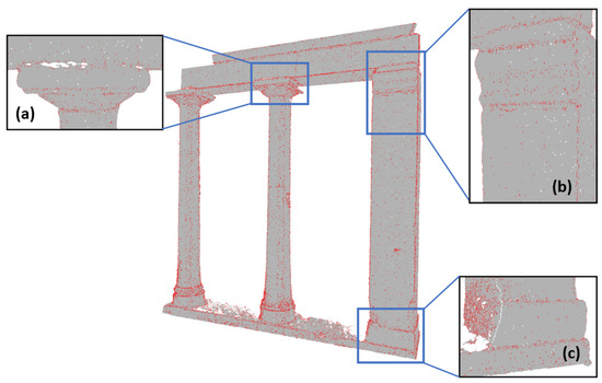
Figure 9.
Visualization of the finite edges on the triangular mesh surface of the Temple of Demeter’s facade. (a,b) Regions where the detected finite edges are densely concentrated in specific sections of the mesh. (c) Region exhibiting a high density of finite edges, primarily due to surface anomalies.
As can be seen in Figure 9, the detected finite edges are more densely concentrated in sections of the mesh where edges are present, such as in the architrave of the temple. However, there are also areas where the finite edges do not correspond to any real edge and have been created due to noise present or due to roughness caused by the wear of the original surface. A typical example of that is the stylobate (Figure 9c), which has suffered significant erosion and shows visible cracks. Consequently, many finite edges have been detected on its surface.
In the following stage, the optimal line segments (Figure 10) that best fit the grouped finite edges were identified using the least squares method.
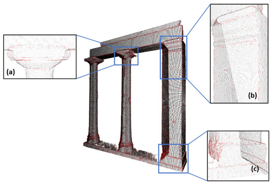
Figure 10.
Visualization of line segments in the dense point cloud of the Temple of Demeter’s facade. (a,b) Regions where the line segments are densely concentrated in sections of the mesh. (c) Region exhibiting many line segments, primarily due to surface anomalies.
In the final step of the algorithm’s implementation, the final 3D edges of the monument were identified using the proposed variation of RANSAC. On the largest surface of the temple (Figure 11a,b), the detected edges accurately represent its geometry.

Figure 11.
Visualization of the final 3D edges of Demeter’s temple. (a,b) Regions where the detected edges accurately represent the temple’s geometry, (c) Region with some wrong detected edges. The numbers indicate different sections on the temple: (1) horizontal geison, (2) architrave, (3a) upper section of the pillar, (3b) lower section of the pillar, (4) stylobate and (5) foundation.
However, in some regions, certain discrepancies were observed between the detected edges and the expected ones. For example, the detected edge on the architrave (2) (Figure 11) is divided into two segments, which do not continue across the entire area above the capitals and show a slight slope towards the upper part of the temple. The discontinuity between the two edges arises due to the gaps in the original triangular mesh, caused by the lower point density in those areas. Additionally, the slope was created during the merging, by RANSAC, from the line segments detected along this edge, as the line segments above the capitals were located at a slightly higher position due to the gaps on the mesh surface. What is more, in the lower section of the pillar (3b) and the stylobate (4) (Figure 11c), there is some damage to the stones with some pieces having fallen off. This causes the creation of scattered edges along these parts of the surface. It is also important to note that between the stylobate (4) and the foundation (5), where there were no problems either with the point cloud or with the triangular mesh, the detected final 3D edges are very close to reality.
As mentioned earlier, the quality of the triangular mesh has a significant impact on the results as it affects the reliability of the detected edges. To understand the extent to which the mesh anomalies affect the results, a region of the monument’s triangular mesh was selected, where gaps were present (Figure 6a). In this specific area, the edge between the temple’s capital and the architrave was not detected along its entire length; instead, two separate edges emerged from the implementation of the algorithm (Figure 12).
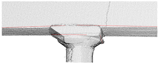
Figure 12.
The final 3D edge is detected in segments before processing the triangular mesh.
For this area, further manual processing of the triangular mesh was carried out to cover the gaps that resulted from the automated execution of the ball-pivoting algorithm [35]. Then, the proposed algorithm was utilized again for that specific area of the monument. As a result, full length of the edge was detected (Figure 13) without any discontinuity.
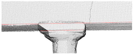
Figure 13.
The final 3D edge is detected along its entire length after processing the triangular mesh.
This experiment demonstrates the significant influence of the quality of the triangular mesh on the reliability of the detected edges and confirms that improving the triangular mesh results in more precise outcomes.
5. Discussion and Future Work
Throughout the development of the proposed algorithm, several challenges were encountered and addressed to ensure the reliability of the final product.
Firstly, a significant challenge was the non-uniform density and unknown noise levels in real-world point clouds. Therefore, for each point cloud, the average density was calculated using the nearest neighbor technique. However, the variability in density and noise made it impractical to establish a definitive minimum density threshold for reliable results. For this reason, synthetic point clouds were created to study the effect of noise and density on the algorithm’s effectiveness. Experiments revealed that, for constant noise levels, increasing point cloud density improved reliability. Conversely, for constant densities, higher noise levels or greater noise standard deviations significantly reduced reliability.
Another critical issue was the long execution time needed for the algorithm’s final stage, which utilized a RANSAC variant. Initially, processing a 32,000-point cloud required over three hours. This was resolved by incorporating a k-D tree structure, reducing execution time to just two minutes.
What is more, the quality of the triangular mesh was found to significantly affect the reliability of results. Gaps or errors in the mesh compromised the accuracy of the detected edges. Improving mesh quality, such as by pre-filtering the point cloud to reduce noise, could enhance the algorithm’s performance. For instance, ref. [38] proposes a noise-reduction method that classifies isolated points as noise based on their average distance from k-nearest neighbors, discards noisy groups that exceed a defined threshold, and produces a cleaner point cloud for better mesh generation.
Apart from the changes that have been made, there are also other interesting suggestions for how research could proceed in the future to upgrade the products of the proposed algorithm. The algorithm can detect edgelets, i.e., small parts of the straight edges present in the point cloud data. The interpolation needed to combine some of these to a longer, more realistic, straight edge might lead to small number of edges being missed. On the other hand, and due to the wear of the surface, there is always a small possibility that a non-existent edge might be detected. Therefore, until a quality control method has been incorporated into the algorithm, the results should be manually examined.
An interesting suggestion that could improve the proposed algorithm and make the process more user-friendly would be the automatic calculation of the minimum density required for the initial cloud to produce a reliable result. This minimum density varies for each cloud and depends on the noise level and standard deviation. The noise percentage could be easily determined by finding the number of noise points using methods like those suggested by [38], while the standard deviation could be calculated from a variance table that represents the average distance of noise points from the other points in the cloud [39]. Subsequent experiments could establish how density, noise, and noise standard deviation interact, enabling thresholds to be set for minimum density requirements based on point cloud characteristics.
Quantitative results of this research are based on synthetic data, as our real-world data lacked ground truth measurements. Thus, it is recommended that ground truth edges are generated through the manual vectorization of the real data in the future. These manually derived edges could then be compared with the automatically detected edges to evaluate the accuracy of the results for the different datasets.
Finally, as far as the literature is concerned, curved edge detection has so far not yet been tackled, as it is an even more complicated problem compared to straight edge detection. However, it would be valuable to explore the possibility of developing methods for identifying curved edges, as this could significantly enhance the versatility of edge detection algorithms in various applications.
6. Conclusions
The proposed method focuses on the detection of edges within point clouds, utilizing the differences in the slopes of normal vectors corresponding to adjacent planes. The developed five-stage algorithm was evaluated using both synthetic and real-world data to assess its performance and robustness across various scenarios. By incorporating a range of techniques, the proposed algorithm effectively addresses challenges related to noise, point cloud irregularities, and computational efficiency, improving the straight edge detection process. Consequently, the results obtained are both satisfactory and align with the original objectives.
Author Contributions
Conceptualization, A.G. and M.P.; methodology, M.P., A.G., A.M. and T.B.; software, A.M.; validation, A.M., T.Β. and M.P.; resources, A.G.; writing—original draft preparation, A.M., A.G., T.B. and M.P.; writing—review and editing, A.M., T.B., A.G. and M.P.; supervision, M.P. and A.G. All authors have read and agreed to the published version of the manuscript.
Funding
This work was partially funded by the European Union’s Horizon 2020 research and innovation programme FELICE (GA no. 101017151) and the Horizon Europe programme SOPRANO (GA no. 101120990).
Data Availability Statement
The data used for the experimental work of this research belong to the authors.
Conflicts of Interest
The authors declare no conflicts of interest.
Notes
| 1 | The process should be executed in a sequential and linear manner, with each step carefully followed to ensure the desired results are achieved. |
| 2 | The percentage of correctly detected edges is determined by comparing the automatically detected edges with the ground truth edges of the synthetic data. |
References
- Abdellali, H.; Frohlich, R.; Vilagos, V.; Kato, Z. L2D2: Learnable line detector and descriptor. In Proceedings of the 2021 International Conference on 3D Vision (3DV), London, UK, 1–3 December 2021. [Google Scholar]
- Zhang, H.; Luo, Y.; Qin, F.; He, Y.; Liu, X. Elsd: Efficient line segment detector and descriptor. In Proceedings of the International Conference on Computer Vision (ICCV), Montreal, QC, Canada, 10–17 October 2021. [Google Scholar]
- Bode, L.; Weinmann, M.; Klein, R. BoundED: Neural boundary and edge detection in 3D point clouds via local neighborhood statistics. ISPRS J. Photogramm. Remote Sens. 2023, 205, 334–351. [Google Scholar] [CrossRef]
- Ye, Y.; Yi, R.; Gao, Z.; Cai, Z.; Xu, K. Delving Into Crispness: Guided Label Refinement for Crisp Edge Detection. IEEE Trans. Image Process. A Publ. IEEE Signal Process. Soc. 2023, 32, 4199–4211. [Google Scholar] [CrossRef] [PubMed]
- Ahmed, M.; Tan, Y.Z.h.i.; Chew, C.; Al-Mamun, A.; Wong, F. Edge and Corner Detection for Unorganized 3D Point Clouds with Application to Robotic Welding. In Proceedings of the 2018 IEEE/RSJ International Conference on Intelligent Robots and Systems (IROS), Madrid, Spain, 1–5 October 2018; pp. 7350–7355. [Google Scholar] [CrossRef]
- Pateraki, M.; Baltsavias, E. Surface discontinuity modelling by LSM through patch adaptation and Use of edges. In Proceedings of the ISPRS Congress, IAPRS, Istanbul, Turkey, 12–23 July 2004; Volume 35, Part B3. pp. 522–527. [Google Scholar]
- Cosgrove, C.; Yuille, A.L. Adversarial Examples for Edge Detection: They Exist, and They Transfer. In Proceedings of the IEEE Winter Conference on Applications of Computer Vision (WACV), Snowmass, CO, USA, 1–5 March 2020; pp. 1059–1068. [Google Scholar] [CrossRef]
- Krizhevsky, A.; Sutskever, I.; Hinton, G.E. Imagenet classification with deep convolutional neural networks. In Proceedings of the 26th Intl. Conf. on Neural Information Processing Systems (NIPS’12), Curran Associates Inc., Lake Tahoe, NV, USA, 3-6 December 2012; pp. 1097–1105. [Google Scholar]
- Agrafiotis, P.; Talaveros, G.; Georgopoulos, A. Orthoimage-to-2D Architectural Drawing with Conditional Adversarial Networks. In ISPRS Annals of the Photogrammetry, Remote Sensing and Spatial Information Sciences; Copernicus Publications: Göttingen, Germany, 2023; pp. 11–18. [Google Scholar] [CrossRef]
- Betsas, T.; Georgopoulos, A.; Doulamis, A. INCAD: 2D Vector Drawings Creation using Instance Segmentation. Int. Arch. Photogramm. Remote Sens. Spat. Inf. Sci. 2024, 48, 65–72. [Google Scholar] [CrossRef]
- Sobel, I.; Feldman, G. A 3x3 isotropic gradient operator for image processing. A Talk Stanf. Artif. Proj. 1968, 1968, 271–272. [Google Scholar]
- Prewitt, J.; Mendelsohn, M.L.; Melville, J.R. The Prewitt operator for detecting edges. IEEE Trans. Comput. 1970, C-19, 313–319. [Google Scholar]
- Canny, J.F. Finding Edges and Lines in Images; Technical Report; Massachusetts Inst of Tech Cambridge Artificial Intelligence Lab: Cambridge MA, USA, 1983. [Google Scholar]
- Canny, J.F. A computational approach to edge detection. IEEE Trans. Pattern Anal. Mach. Intell. 1986, PAMI-8, 679–698. [Google Scholar] [CrossRef]
- Grompone Von Gioi, R.; Jakubowicz, J.; Morel, J.M.; Randall, G. LSD: A fast line segment detector with a false detection control. IEEE Trans. Pattern Anal. Mach. Intell. (PAMI) 2008, 32, 722–732. [Google Scholar] [CrossRef]
- Akinlar, C.; Topal, C. EDLines: A real-time line segment detector with a false detection control. Pattern Recognit. Lett. 2011, 32, 1633–1642. [Google Scholar] [CrossRef]
- Suarez, F.; Smith, J.; Zhang, L. ELSED Algorithm: An Enhanced Edge Detection Technique for Image Processing. J. Image Process. Comput. Vis. 2022, 15, 123–134. [Google Scholar]
- Xie, Y.; Tian, J.; Zhu, X.X. Linking points with labels in 3D: A review of point cloud semantic segmentation. IEEE Geosci. Remote Sens. Mag. 2020, 8, 38–59. [Google Scholar] [CrossRef]
- Poma, X.S.; Riba, E.; Sappa, A. Dense extreme inception network: Towards a robust CNN model for edge detection. In Proceedings of the IEEE/CVF Winter Conference on Applications of Computer Vision, Snowmass Village, CO, USA, 1–5 March 2020; pp. 1923–1932. [Google Scholar]
- Su, Z.; Liu, W.; Yu, Z.; Hu, D.; Liao, Q.; Tian, Q.; Pietikainen, M.; Liu, L. Pixel difference networks for efficient edge detection. In Proceedings of the IEEE/CVF International Conference on Computer Vision, Montreal, BC, Canada, 11–17 October 2021; pp. 5117–5127. [Google Scholar]
- Dhankhar, P.; Sahu, N. A Review and Research of Edge Detection Techniques for Image Segmentation. Int. J. Comput. Sci. Mob. Comput. 2013, 2, 86–92. [Google Scholar]
- Lu, X.; Liu, Y.; Li, K. Fast 3D Line Segment Detection from Unorganized Point Cloud. arXiv 2019, arXiv:abs/1901.02532. [Google Scholar]
- Rodríguez Miranda, Á.; Valle Melón, J.M.; Martínez Montiel, J.M. 3D Line Drawing from Point Clouds using Chromatic Stereo and Shading. Digital Heritage. In Proceedings of the 14th International Conference on Virtual Systems and Multimedia VSMM, Limassol, Cyprus, 20–25 October 2008; pp. 77–84, ISBN 978-963-8046-99-4. [Google Scholar]
- Canciani, M.; Falcolini, C.; Saccone, M.; Spadafora, G. From Point Clouds to Architectural Models: Algorithms for Shape Reconstruction. In Proceedings of the International Archives of the Photogrammetry, Remote Sensing and Spatial Information Sciences, Volume XL-5/W1, 20133D-ARCH 2013—3D Virtual Reconstruction and Visualization of Complex Architectures, Trento, Italy, 25–26 February 2013. [Google Scholar]
- Briese, C.; Pfeifer, N. Towards automatic feature line modelling from terrestrial laser scanner data. Int. Arch. Photogramm. Remote Sens. Spat. Inf. Sci. 2008, 37, 463–468. [Google Scholar]
- Nguatem, W.; Drauschke, M.; Mayer, H. Localization of Windows and Doors in 3d Point Clouds of Facades. ISPRS Ann. Photogramm. Remote Sens. Spat. Inf. Sci. 2014, 2, 87–94. [Google Scholar] [CrossRef]
- Mitropoulou, A.; Georgopoulos, A. An Automated Process to Detect Edges in Unorganized Point Clouds. ISPRS Ann. Photogramm. Remote Sens. Spat. Inf. Sci. 2019, 4, 99–105. [Google Scholar] [CrossRef]
- Liakopoulou, A.M. Development of a Plane Intersection Algorithm for 3D Edge Determination. Diploma Thesis, Lab of Photogrammetry, NTUA (in Greek). 2022. Available online: https://dspace.lib.ntua.gr/xmlui/handle/123456789/56782 (accessed on 5 May 2024).
- Bazazian, D.; Casas, J.R.; Ruiz-Hidalgo, J. Fast and Robust Edge Extraction in Unorganized Point Clouds. In Proceedings of the International Conference on Digital Image Computing: Techniques and Applications (DICTA), Adelaide, SA, Australia, 23–25 November 2015; pp. 1–8. [Google Scholar] [CrossRef]
- Dolapsaki, M.M.; Georgopoulos, A. Edge Detection in 3D Point Clouds Using Digital Images. ISPRS Int. J. Geo-Inf. 2021, 10, 229. [Google Scholar] [CrossRef]
- Bao, T.; Zhao, J.; Xu, M. Step edge detection method for 3D point clouds based on 2D range images. Optik 2015, 126, 2706–2710. [Google Scholar] [CrossRef]
- Betsas, T.; Georgopoulos, A. 3D Edge Detection and Comparison using Four-Channel ImagesS. Int. Arch. Photogramm. Remote Sens. Spat. Inf. Sci. 2022, 48, 9–15. [Google Scholar] [CrossRef]
- Makka, A.; Pateraki, M.; Betsas, T.; Georgopoulos, A. 3D edge detection based on normal vectors. Int. Arch. Photogramm. Remote Sens. Spat. Inf. Sci. 2024, 48, 295–300. [Google Scholar] [CrossRef]
- Aggarwal, A.; Stolkin, R.; Marturi, N. Unsupervised learning-based approach for detecting 3D edges in depth maps. Sci. Rep. 2024, 14, 796. [Google Scholar] [CrossRef] [PubMed]
- Xin, X.; Huang, W.; Zhong, S.; Zhang, M.; Liu, Z.; Xie, Z. Accurate and complete line segment extraction for large-scale point clouds. Int. J. Appl. Earth Obs. Geoinf. 2024, 128, 103728. [Google Scholar] [CrossRef]
- Bernardini, F.; Mittleman, J.; Rushmeier, H.; Silva, C.; Taubin, G. The ball-pivoting algorithm for surface reconstruction. IEEE Trans. Vis. Comput. Graph. 1999, 5, 349–359. [Google Scholar] [CrossRef]
- Betsas, T. Automated Detection of Edges in Point Clouds Using Semantic Information. Diploma Thesis, Laboratory of Photogrammetry, NTUA. Available online: https://dspace.lib.ntua.gr/xmlui/handle/123456789/53090 (accessed on 8 February 2024).
- Balta, H.; Velagic, J.; Bosschaerts, W.; De Cubber, G.; Siciliano, B. Fast Statistical Outlier Removal Based Method for Large 3D Point Clouds of Outdoor Environments. IFAC-Pap. 2018, 51, 348–353. [Google Scholar] [CrossRef]
- Wang, L.; Chen, Y.; Song, W.; Xu, H. Point Cloud Denoising and Feature Preservation: An Adaptive Kernel Approach Based on Local Density and Global Statistics. Sensors 2024, 24, 1718. [Google Scholar] [CrossRef]
Disclaimer/Publisher’s Note: The statements, opinions and data contained in all publications are solely those of the individual author(s) and contributor(s) and not of MDPI and/or the editor(s). MDPI and/or the editor(s) disclaim responsibility for any injury to people or property resulting from any ideas, methods, instructions or products referred to in the content. |
© 2025 by the authors. Licensee MDPI, Basel, Switzerland. This article is an open access article distributed under the terms and conditions of the Creative Commons Attribution (CC BY) license (https://creativecommons.org/licenses/by/4.0/).