Multi-Scale Forecasting of Natural Rubber Prices Using VMD-Augmented BiLSTM: A Hybrid Architecture Ablation Study

Highlights

What are the main findings?

• The VMD-Augmented BiLSTM framework achieves Pearson correlation of 0.821 ± 0.016 and a Standard Deviation Ratio (StdR) of 1.091 ± 0.060 on daily rubber price changes across five random seeds, with directional accuracy of 82.5% ± 1.8% and down-direction recall of 78.1% ± 5.5% on a leakage-free held-out test set.
• Directional accuracy alone is an insufficient evaluation metric for differenced commodity series: Vanilla LSTM attains directional accuracy of 82.29% ± 0.00 across five seeds, statistically indistinguishable from that of the proposed model, yet exhibits variance collapse (StdR = 0.210 ± 0.007 vs. 1.091 ± 0.060), confirming the need for variance-sensitive co-primary metrics.

What are the implications of the main findings?

• Appending VMD components directly as input features—rather than summing independent mode forecasts—preserves multi-scale frequency information and prevents variance collapse (per-IMF conventional ablation: StdR ≈ 0.20) on differenced price series.
• Ablation analysis indicates that the bidirectional LSTM pathway is the primary architectural driver of performance; the additional Transformer self-attention pathway offers no consistent gain in this context.

Abstract

This study examines whether decomposition-based deep learning forecasts of daily changes in natural rubber prices can appear directionally accurate while failing to preserve the dispersion of the target series—a failure mode that conventional accuracy metrics cannot detect. Using daily RSS3 FOB price changes in the period 2018–2026, a VMD-Augmented BiLSTM forecasting design is employed as the empirical vehicle for testing this question. Forecasts are evaluated jointly through Pearson correlation, directional accuracy, class-conditional recall, and the Standard Deviation Ratio (StdR), with StdR serving as a diagnostic for variance collapse on differenced series. The deployed model appends all Variational Mode Decomposition (VMD) components directly to the economic feature matrix and feeds the augmented sequence into a bidirectional LSTM encoder with temporal attention; VMD is fitted using an expanding-window procedure to prevent information leakage. The design is compared to a conventional per-IMF decomposition–forecast pipeline, a Vanilla LSTM, ARIMA(2,0,2), and a dual-pathway BiLSTM–Transformer control. On a 175-observation deduplicated test set, the deployed model attains Pearson correlation of $r=0.821\pm 0.016$, directional accuracy of $82.5\%\pm 1.8\%$, and StdR $=1.091\pm 0.060$ across five random seeds. The Vanilla LSTM baseline attains directional accuracy of $82.29\%\pm 0.00$—statistically indistinguishable from that of the deployed model—yet exhibits variance collapse (StdR $=0.210\pm 0.007$), confirming that DA alone cannot distinguish predictive skill grounded in conditional dynamics from forecasts that merely reproduce the unconditional sign distribution. The principal contribution is methodological: A variance-sensitive evaluation protocol that distinguishes forecast skill grounded in conditional dynamics from directional but underdispersed predictions, demonstrated across three empirically distinct mechanisms by which variance collapse arises in this setting.

1. Introduction

Natural rubber is a critical industrial input and a strategic agricultural commodity that plays a central role in global manufacturing supply chains; it is widely used in tires, medical gloves, engineering components, and a broad range of technical rubber products. Global production is highly concentrated in Southeast Asia, particularly Thailand, Indonesia, and Malaysia, which, together, account for the majority of the global supply [1,2]. Thailand has consistently remained the world’s leading exporter of natural rubber: in 2025, it produced approximately 4.79 million tonnes (32.18% of global production), with about 85.79% of output exported to international markets [3]. Price volatility in natural rubber markets therefore carries direct consequences for the income of millions of smallholder farmers and for the cost structure of downstream industries that rely heavily on rubber-based inputs.

Natural rubber prices are jointly driven by agricultural seasonality, macroeconomic conditions, exchange rate dynamics, and speculative activity in futures markets, producing dynamics that are simultaneously non-linear, non-stationary, and subject to structural breaks [4,5,6]. Ribbed Smoked Sheet No. 3 (RSS3) serves as the benchmark grade for international transactions, with export prices typically quoted on a Free on Board (FOB) basis at major Thai ports. Cross-market price co-movement among SHFE, SGX, and JPX (TOCOM) futures provides additional predictive content beyond domestic spot prices alone, motivating the inclusion of exchange-traded settlement prices as model inputs [7]. This informational structure is asymmetric: Sang and Ma [8] demonstrate that SHFE Granger-causes TOCOM but not vice versa, while Kepulaje et al. [9] (pp. 159–161) show that SGX RSS3 Rubber Futures (SRU) and SGX TSR20 Rubber Futures (STF) predict regional spot prices more consistently than TOCOM/JPX Rubber Futures (JRU) do—implying that the futures exchanges operate as a layered rather than flat information system, with the informational weight of each venue depending on whether one is studying financial benchmarking or physical export pricing.

Commodity price forecasting has long relied on econometric models such as ARIMA, VAR, and GARCH, which provide well-established frameworks for capturing temporal dependencies and volatility structures [10,11]. In the literature on natural rubber, this lineage is exemplified by Zahari et al. [12], who apply the Box–Jenkins procedure to Malaysian SMR20 and identifies ARIMA(1,1,0) as the best-fitting model, and by Khin and Thambiah [13], who show that a simultaneous supply–demand–price system outperforms univariate ARIMA across RMSE, MAE, and information criteria—demonstrating that purely univariate extrapolation is insufficient once market structure is made explicit. The linearity assumptions underlying these methods, however, limit their capacity on series with structural breaks and high non-stationarity, characteristics that are particularly pronounced in energy and agricultural commodity prices [14,15]. Subsequent studies introduced machine learning methods including support vector machines (SVMs), multi-layer perceptrons (MLPs), random forests, extreme gradient boosting (XGBoost), and back-propagation neural networks [16,17,18], alongside hybrid statistical–machine learning frameworks such as ARIMA–SVM [19,20]. These methods address non-linearity but remain limited in capturing long-range dependencies, motivating the adoption of deep learning–based alternatives.

Since the above-mentioned machine learning studies, deep recurrent architectures—particularly Long Short-Term Memory (LSTM), Gated Recurrent Unit (GRU), and Bidirectional LSTM (BiLSTM) architectures—have become standard for sequential modelling, and they outperform classical benchmarks in energy demand prediction, financial market forecasting, and environmental time-series modelling [21,22,23]. BiLSTM extends conventional LSTM by processing sequences simultaneously in forward and backward directions, integrating contextual information from both past and future states within the observation window; this yields richer temporal representations in environments characterised by strong seasonality, non-linear interactions, and abrupt fluctuations [24]. For natural rubber specifically, Phoksawat et al. [25] demonstrate that a multi-layer LSTM achieves 95.88% accuracy on Thai RSS3 prices, while Eng and Khalid [26] confirm that LSTM outperforms ARIMA on Malaysian SMR20 across MAE, RMSE, and MAPE—with both studies noting that further gains require the explicit incorporation of exogenous drivers such as exchange rates, energy prices, and futures markets. Hybrid extensions of BiLSTM include CNN–BiLSTM architectures that combine local feature extraction with bidirectional temporal learning [27,28], attention mechanisms that emphasise the most informative time steps [29], and meta-heuristic or gradient-boosting combinations that capture residual non-linear patterns. These hybrids remain limited, however, in their ability to separate and individually model components operating across distinctly different temporal scales—a constraint that is particularly consequential for commodity series with co-existing trend, cyclical, and noise dynamics.

A parallel research direction addresses this limitation by incorporating signal decomposition—Empirical Mode Decomposition (EMD), Variational Mode Decomposition (VMD), Wavelet Transform (WT), or Seasonal-Trend Decomposition using LOESS (STL)—as a preprocessing stage, separating the original series into components representing distinct frequency structures and thereby reducing non-stationarity [7,29,30]. Decomposition-based hybrid frameworks (EMD–LSTM, VMD–LSTM, VMD–GRU, VMD–TCN–LSTM, and STL–LSTM) have been shown to improve forecasting accuracy across coal, solar, wind, and electricity-load applications [29], with VMD-based models outperforming both single-model and earlier decomposition-based alternatives [31,32]. Combining VMD with attention-based sequence architectures yields complementary improvements: VMD decomposes complex series into more learnable components, while attention enhances the selection of informative features and time steps [33] (pp. 922–923); recent FX-forecasting evidence further indicates that VMD-enhanced bidirectional recurrent architectures can materially improve out-of-sample performance on low-frequency financial series [34]. Within natural rubber, VMD extracts economically meaningful multi-scale components, and bidirectional recurrent architectures improve both fitting and directional prediction; importantly, the predictive value of individual modes depends on their time-scale correspondence with the forecast target [7] (p. 6). More recently, Transformer-based architectures—Informer, Autoformer, FEDformer, PatchTST, and ReVIN—have introduced sparse attention, decomposition-based encoders, frequency-enhanced representations, patch-level embedding, and distribution-shift normalisation, substantially improving long-sequence forecasting [33,35,36,37]. A parallel line of work questions whether this architectural complexity is necessary at horizons of operational interest: Zeng et al. [38] introduce DLinear, a simple linear decomposition baseline reported to match or outperform Informer, Autoformer, and FEDformer on standard benchmarks, and subsequent work—SOFTS [39], MoFo [40], and patch-based hierarchical-attention variants such as PHAT [41]—continues this trajectory toward parsimonious alternatives. The contribution of the present work operates at the level of preprocessing and evaluation methodology and is therefore composable with these alternative downstream architectures; a systematic backbone comparison is identified as a natural follow-up in Section 5.

A common limitation of existing decomposition-based pipelines is that signal separation is treated purely as a preprocessing step to improve input quality, after which each intrinsic mode function is forecast independently and the predictions summed. This per-IMF-and-sum design is prone to a forecast-output underdispersion problem on stationary (differenced) commodity series: under symmetric loss and limited predictive information, regression models shrink predictions toward the conditional mean, reducing MAE and RMSE while suppressing the variance of the predicted series. The mechanism is conceptually related to but distinct from the recursive training-data collapse discussed by Shumailov et al. [42] (pp. 755–757); the shared element is the systematic erosion of output variance under compound or underdetermined estimation, while the present application refers strictly to forecast-output dispersion on differenced commodity series rather than to recursive training-data degradation. Rajpal et al. [43] (pp. 13–15) document the directly analogous output-level pathology in financial forecasting, showing that symmetric loss objectives push models toward degenerate, one-sided prediction regimes whose apparent performance masks near-zero predictive content. In the context of natural rubber, Fakthong et al. [44] further argue that existing studies are heavily oriented toward short-term fluctuation tracking and that limited attention has been paid to architectures that preserve multi-scale information.

This study, using a 24-feature economic input set for the period 2018–2026, examines whether decomposition-based deep learning forecasts of daily RSS3 FOB price changes can appear directionally accurate while failing to preserve the dispersion of the target series. Three contributions follow. First, the study shows that the conventional per-IMF forecasting-and-summation pipeline can induce variance collapse on differenced rubber prices (per-IMF ablation: StdR ≈ 0.20) and that appending VMD components as auxiliary features within a single BiLSTM encoder preserves amplitude fidelity more effectively. Second, the study establishes a variance-sensitive evaluation protocol in which directional accuracy is interpreted jointly with Pearson correlation, the Standard Deviation Ratio (StdR), and class-conditional recall; the protocol’s diagnostic power is demonstrated across three empirically distinct mechanisms by which variance collapse arises—feature deficiency (Stage 1 vs. Stage 2 cross-stage analysis), compound estimation error (per-IMF pipeline ablation), and underparameterised recurrent learning (a Vanilla LSTM baseline that attains directional accuracy statistically indistinguishable from that of the deployed model yet exhibits StdR $=0.210\pm 0.007$). Third, the cross-stage feature-availability analysis serves as a design check for the Stage 3 evaluation protocol. The theoretical basis for this metric combination is established by Taylor [45] (pp. 7183–7184), who demonstrate that correlation and the Standard Deviation Ratio are complementary rather than substitutable descriptors of forecast skill: correlation measures co-movement in shape, while StdR measures amplitude fidelity, and a reduction in RMS error cannot be taken as evidence of improved skill if forecast variance has been suppressed in the process. This evaluation logic aligns with a broader methodological literature: Bürgi [46] shows that DA is not self-sufficient without knowledge of magnitude sensitivity and user objective; McCarthy and Snudden [47] (pp. 1–7) demonstrate that temporal aggregation can mechanically inflate success ratios beyond 0.5 even for a random walk, generating pseudo-skill where no genuine predictability exists; and Costantini and Kunst [48] show that embedding DA into model-selection criteria seldom yields robust gains and can worsen MSE performance—together implying that DA should function as a supplementary diagnostic rather than a primary evaluation objective [49].

The remainder of the paper is organised as follows. Section 2 describes the data, preprocessing pipeline, decomposition procedure, model architecture, and evaluation protocol. Section 3 reports the empirical results. Section 4 discusses the economic interpretation and practical implications. Section 5 concludes with limitations and directions for future research.

2. Materials and Methods

This section describes the data, preprocessing pipeline, and architecture of the proposed VMD-Augmented BiLSTM forecasting framework. Section 2.1 motivates the primary analytical sample through a cross-stage comparison. Section 2.2, Section 2.3, Section 2.4 and Section 2.5 describe, respectively, data and feature construction, model architecture, training configuration, and evaluation protocol.

2.1. Cross-Stage Comparison and Rationale for the Primary Analytical Sample

The full dataset (2 October 1999–27 February 2026, $n=7492$ daily observations) is structured into three chronological stages defined by input feature availability. Stage 1 (21 April 2003–30 December 2014, $n=3030$) includes 11 features comprising domestic rubber spot prices, cup-lump prices, USS prices, and exchange-traded futures (JPX and SHFE), covering a period before foreign exchange, energy, and macroeconomic series became available. Stage 2 (1 January 2015–4 May 2018, $n=872$) extends coverage to 22 features following the availability of USD/THB, CNY/THB, USD/CNY, Brent, WTI, China PMI Manufacturing, Baltic Dry Index, and ENSO ONI data. Stage 3 (7 May 2018–27 February 2026, $n=2675$ observations) represents the first period with complete coverage of all 24 input features, including SGX RSS3 and TSR20 settlement prices, and constitutes the primary analytical sample for this study. To assess the sensitivity of model performance to input feature availability, the VMD-Augmented BiLSTM was trained and evaluated independently on all three sub-samples using only the features available within each period. All models were evaluated on held-out test partitions of their respective datasets using an identical protocol.

Prior to model training, VMD was applied to the training partition only within each sub-sample to determine the optimal number of modes K. For validation and test partitions, VMD was re-applied using an expanding-window procedure anchored at the training start date, ensuring that no future observation informed the decomposition at any forecasting point. Stage 1 yields a highly concentrated energy distribution under K = 5, with IMF1 accounting for 95.3% of total signal variance—indicating that the pre-2015 rubber market was dominated by a single low-frequency trend, consistent with the sustained commodity super-cycle of 2003–2011 followed by a sharp price correction. Stage 2 requires K = 7 to adequately capture signal complexity, with energy distributed more evenly across seven components (range: 7.6–23.9%), reflecting the heightened multi-frequency dynamics of the 2015–2018 transition period. Stage 3 under K = 6 presents a structured decomposition: IMF1 retains dominance at 74.7%, with secondary components carrying economically interpretable energy shares (IMF2 = 11.5%; IMF3 = 5.6%; IMF4 = 2.7%; IMF5 = 2.5%; IMF6 = 3.1%); full decomposition results for Stage 3 are presented later in Section 3.2. This cross-stage analysis demonstrates that the frequency structure of RSS3 prices is non-stationary across market regimes and that K = 6 (selected via grid search on the training partition only) is the appropriate decomposition depth for Stage 3.

Out-of-sample performance results are summarised in

Table 1. Cross-stage out-of-sample performance—VMD-Augmented BiLSTM. The Stage 3 row is reported as the multi-seed mean to provide a directly comparable performance benchmark for use throughout the main analysis (Section 3.4).

Stage	n (Test)	Input Features	Test-Set Metrics (Differenced Series)
			MAE	RMSE	Pearson’s r	StdR
Stage 1 (2003–2014)	283	11	0.036	0.050	0.38	0.34
Stage 2→3 (22 features; Stage 3 test window)	247	22	0.044	0.075	0.12	0.11
Stage 3 (2018–2026) ✓	175	24	$0.339\pm 0.023$	$0.456\pm 0.035$	$0.821\pm 0.016$	$1.091\pm 0.060$

Notes: Metrics are computed on the first-differenced RSS3 FOBm1 series (Baht/kg/day) after inverse min–max transformation. Stage 1 and Stage 2→3 are reported as single-seed reference configurations from the early-stage feasibility analysis; Stage 3 is reported as the multi-seed mean ± 1 SD across 5 seeds $\{7,42,123,999,2024\}$ to match the protocol of the primary results (Section 3.4). Cross-stage differences in absolute MAE/RMSE reflect both differences in test partitions and differences in evaluation protocols; the row-wise comparison should accordingly be read primarily through the scale-invariant Pearson r and StdR columns. Stage 2→3 denotes a model trained on Stage 2 features and evaluated on the Stage 3 test partition to allow direct feature-set comparison. Directional accuracy is not reported in this table because the Stage 1 and Stage 2 early-stage feasibility runs used a different directional denominator from the deduplicated primary protocol of Section 3.4; the cross-stage comparison is therefore interpreted only through Pearson’s r and StdR. ✓ denotes the primary analytical sample used in all subsequent analyses.

. Stage 3 shows the strongest performance on the scale-invariant co-primary diagnostics, Pearson’s r and StdR; MAE and RMSE are not directly comparable across stages because the partitions, evaluation windows, and reporting protocols differ. The most discriminating indicator is the Pearson correlation between predicted and realised price changes: Stage 3 achieves $r=0.821\pm 0.016$ (multi-seed, under the leakage-free pipeline), compared with $r=0.38$ for Stage 1 and $r=0.12$ for Stage 2 evaluated on the Stage 3 test window. The Standard Deviation Ratio (StdR), which equals 1.0 under ideal forecast dispersion and is invariant to unit scaling, further reveals that Stage 1 (StdR = 0.34) and Stage 2 (StdR = 0.11) both exhibit pronounced variance collapse: the model defaults toward near-zero predictions, capturing directional frequency but suppressing magnitude entirely. Stage 3 achieves StdR $=1.091\pm 0.060$, confirming that the full feature set enables the model to reproduce the dispersion of the target series. Directional accuracy is not reported in Table 1 because the Stage 1 and Stage 2 early-stage feasibility runs used a different directional denominator (raw test windows without the multi-contract deduplication applied in the primary protocol of Section 3), and were not designed for cross-stage DA comparison. The cross-stage comparison is therefore conducted exclusively through the scale-invariant Pearson’s r and StdR diagnostics, in line with the benchmark-sensitivity problem documented by Bürgi [46] (pp. 7909–7910): when class composition is skewed and the underlying series is highly persistent, DA can remain nominally high across radically different model configurations while conveying no information about whether the model captures conditional dynamics—a limitation that StdR and Pearson’s r directly address.

These results provide two complementary pieces of evidence supporting the study design. First, the stepwise degradation in StdR and Pearson’s r as features are removed confirms that the SGX settlement prices introduced in Stage 3 carry incremental predictive content that is not redundant to the 22 features available in Stage 2. Second, the inability of the Stage 1 and Stage 2 models to reproduce forecast variance—despite achieving high directional accuracy—illustrates a well-known failure mode of deep learning models on stationary differenced series when input information is insufficient: the model learns the unconditional mean rather than the conditional distribution. This pattern is the forecast-output analogue of the underdetermined-estimation failures discussed in the broader literature on distributional collapse [42], pp. 755–757, with the present application referring specifically to underdispersion of the forecast distribution conditional on limited input information rather than to recursive training-data degradation. Stage 3 is thus the minimum sufficient feature set for this forecasting task, and all primary results reported in Section 3 are based on this sub-sample.

2.2. Data, Preprocessing, and Input Features

2.2.1. Target Variable and Stationarity

The study focuses on the Stage 3 sub-sample (7 May 2018–27 February 2026, n = 2675 observations), which represents the first period with complete coverage of all 24 input features, including SGX settlement prices. The target variable is the first-differenced RSS3 FOB near-month price (Baht/kg/day):

$$\Delta p_t=p_t-p_{t-1}$$

(1)

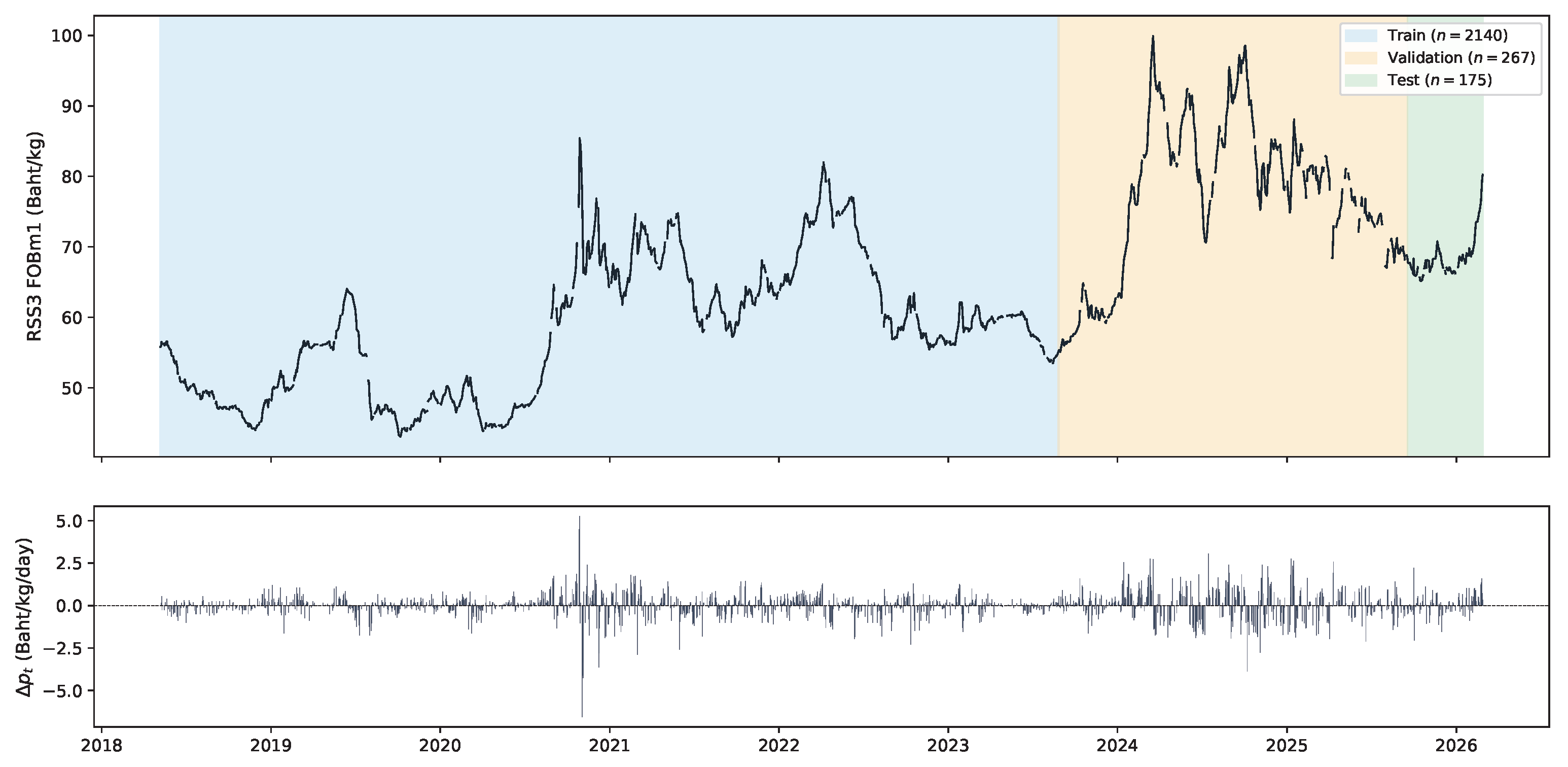
where $p_t$ denotes the RSS3 FOB spot price on day t (Baht/kg). Augmented Dickey–Fuller (ADF) unit root tests confirmed that 21 of the 24 economic features are non-stationary in levels; full ADF results are reported in Appendix B. All non-stationary series were transformed to first-differenced series prior to model input. Descriptive statistics of the differenced target series over the test partition are provided in

Table 2. Descriptive statistics—$\Delta p_t$ (test set, n = 175).

Series	Mean	SD	Min	Max	Skew	Kurtosis
$\Delta p_t$ (Baht/kg/d)	0.01	0.44	−1.98	1.80	−0.18	4.62
$\Delta {\tilde{p}}_t$ (normalised)	0.00	0.08	−0.34	0.31	−0.18	4.62

Notes: ADF test statistic for $\Delta p_t$: −18.73 (p< 0.001). Jarque–Bera test rejects normality (p< 0.001). $\Delta {\tilde{p}}_t$ denotes the normalised version used as model input.

; the corresponding price level and differenced series are visualised in Figure 1. The series exhibits excess kurtosis and mild negative skewness, consistent with stylised facts of commodity price changes.

2.2.2. Data Partitioning

The Stage 3 sub-sample is partitioned chronologically into three non-overlapping sets (

Table 3. Chronological data split—Stage 3.

Partition	Date Range	Observations	Share	Purpose
Training	07-05-2018 → 27-08-2023	2140	80%	Parameter estimation
Validation	28-08-2023 → 17-09-2025	267	10%	Early stopping/LR scheduling
Test	18-09-2025 → 27-02-2026	237 raw/175 effective	∼9%	Out-of-sample evaluation

). The test start date is pinned at 18 September 2025 to ensure comparability with the primary benchmark evaluation. The chronological test window contains 237 raw daily observations; after the removal of duplicated multi-contract entries on identical trading dates according to the evaluation protocol, the effective leakage-free test set used for all primary differenced-space evaluation contains 175 unique observations. The non-zero directional denominator on this effective sample is 151 days (78 up days and 73 down days), with the remaining 24 days having zero realised change. Chronological ordering is strictly preserved to prevent look-ahead bias.

2.2.3. Missing Value Handling and Normalisation

Missing values arising from weekends and public holidays are handled by forward filling (maximum three consecutive days), with remaining gaps filled by linear interpolation (maximum ten days). All features are normalised using a min–max scaler fitted exclusively on the training partition to prevent data leakage:

$$\tilde{x}=2·{\displaystyle \frac{\left(x-x_{min}\right)}{\left(x_{max}-x_{min}\right)}}-1$$

(2)

$$\Delta {\widehat{p}}_t={\displaystyle \frac{{\widehat{y}}_t+1}{2}}·\left(\Delta p_{max}-\Delta p_{min}\right)+\Delta p_{min}$$

(3)

2.2.4. Input Feature Matrix

The input feature matrix comprises 24 economic variables spanning five categories, as summarised in

Table 4. Input feature categories (Stage 3, 24 variables).

Category	Features	Count	Source
Rubber spot and futures	RSS3 FOBm1/m2, STR20 FOBm1/m2, Latex FOBm1/m2, CupLump, USS (all differenced)	8	TRA
Exchange futures	RSS3 JPX m1, RSS3 SHFE m1/m2, RSS3 SGX m1, TSR20 SGX m2 (all differenced)	5	JPX/SHFE/SGX
Exchange rates	USD/THB, CNY/THB, USD/CNY (all differenced)	3	Bloomberg
Energy	Brent diff, WTI diff, Brent return, Brent lag-1 diff	4	EIA/Reuters
Macro/demand	China PMI Manufacturing diff, Baltic Dry Index diff, ENSO ONI diff, COVID dummy	4	CEIC/NOAA/WHO
Total economic variables		24

. These features capture the main demand-side and supply-side drivers of natural rubber prices, including futures markets, foreign exchange rates, energy prices, and macroeconomic indicators. The COVID dummy variable and ENSO ONI are retained in levels; all other features are first-differenced. This variable selection is grounded in the structural rubber forecasting literature: Ref. [50] (pp. 8–9) identifies exchange rates, synthetic rubber prices, GDP growth, crude oil prices, and world stocks as central price determinants in a simultaneous supply–demand framework; Ref. [51] (pp. 1471–1472) confirms through logic-mining variable selection that exports, imports, stocks, exchange rates, and crude oil prices carry the highest predictive weight— providing empirical justification for the multi-category feature design adopted here.

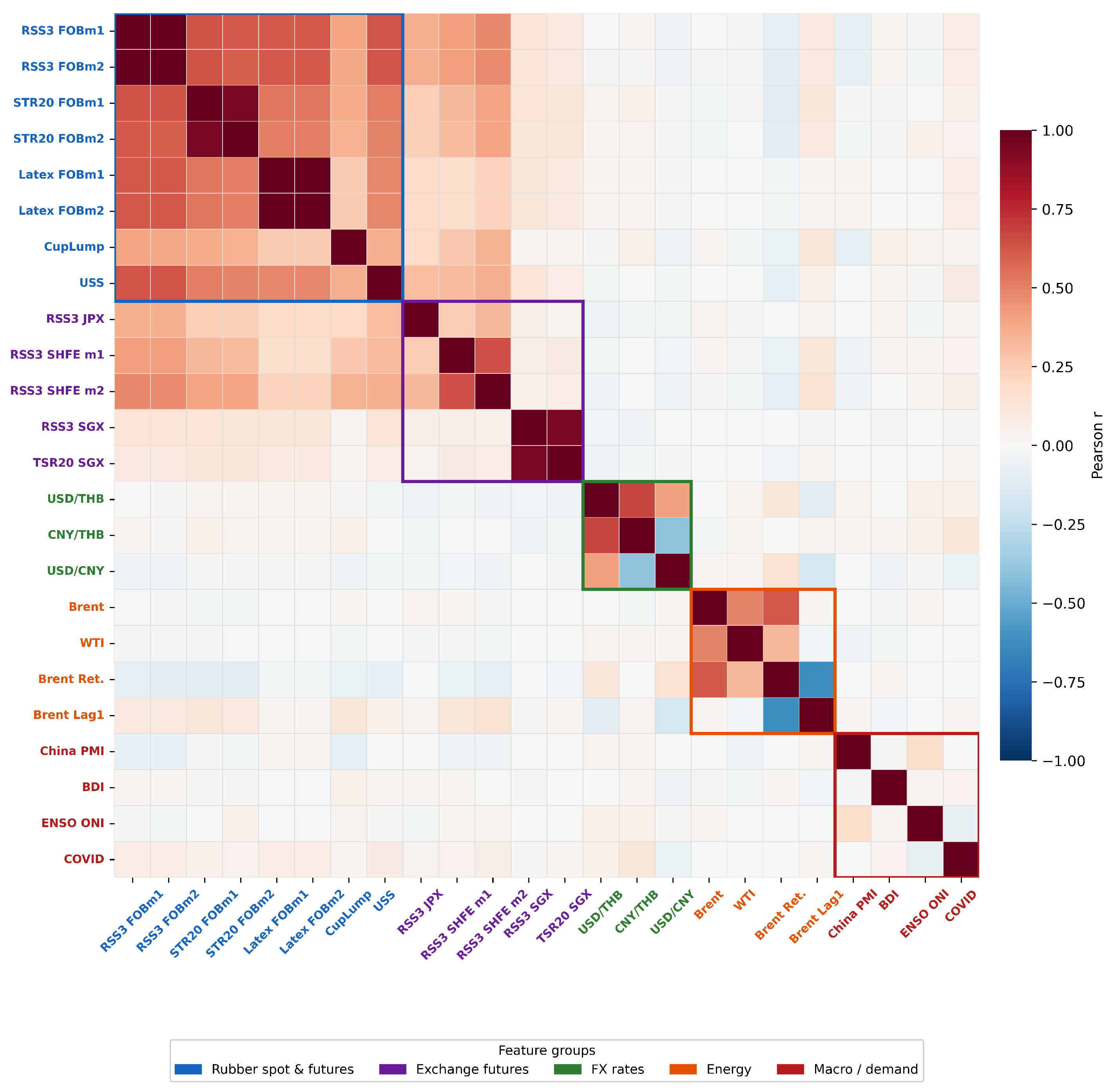
Features are grouped into five clusters in Figure 2: rubber spot price and futures (blue), exchange futures (purple), exchange rates (green), energy (orange), and macro/demand indicators (brown). Within-cluster correlations are substantially higher than cross-cluster correlations, confirming that each feature group captures partially independent information. RSS3 FOBm1 (target variable) shows moderate positive correlation with other rubber futures but near-zero correlation with energy and macro variables in the differenced space. The inclusion of SGX RSS3 and TSR20 settlement prices alongside SHFE and JPX futures is motivated by the transmission evidence from Kepulaje et al. [9] (pp. 159–161), who find that SGX contracts carry greater short-run informational weight in the futures-to-spot transmission equation than TOCOM/JPX Rubber Futures (USS rubber)—and by Pinitjitsamut [52], who shows that FOB Bangkok serves as the operative export-pricing node through which SHFE signals are filtered into domestic Thai prices, making both the exchange and export pricing layers necessary inputs for a complete forecasting system.

2.2.5. VMD Feature Augmentation

Variational Mode Decomposition (VMD), proposed by [53], decomposes a time series into a finite set of band-limited intrinsic mode functions (IMFs) by solving a constrained variational optimisation problem. Unlike Empirical Mode Decomposition (EMD), VMD simultaneously estimates all modes and their centre frequencies by minimising total bandwidth while ensuring that their sum reconstructs the original signal. The optimisation is solved using the Alternating Direction Method of Multipliers (ADMM) [54], pp. 13–20. Empirical evidence across financial and commodity markets confirms that VMD can separate trend, periodic, and disturbance components in non-stationary series, enabling downstream recurrent models to outperform stand-alone econometric and deep learning benchmarks [24]. In commodity-price forecasting specifically, VMD-based hybrid models have been shown to outperform both single-model and earlier decomposition-based alternatives, with further gains when structurally relevant long-run drivers are incorporated into the forecasting system [31].

Let $\Delta p_t$ denote the differenced target series. The VMD objective is to find K modes ${\left\{u_k\right\}}_{k=1}^K$ and their centre frequencies ${\left\{{\omega }_k\right\}}_{k=1}^K$ by solving

$$\begin{array}{cc}\hfill \underset{\left\{u_k\right\},\left\{{\omega }_k\right\}}{min}& {\displaystyle \sum _{k=1}^K}{∥{\partial }_t\left[\left(\delta \left(t\right)+{\displaystyle \frac{j}{\pi t}}\right)\ast u_k\left(t\right)\right]e^{-j{\omega }_{k}t}∥}_2^2\hfill \\ \hfill \mathrm{subject}\mathrm{to}& {\displaystyle \sum _{k=1}^K}{u}_k\left(t\right)=f\left(t\right)\hfill \end{array}$$

(4)

Recent evidence from environmental forecasting further confirms that coupling VMD with sequence models can substantially improve predictive accuracy by separating short- and long-run signal structures before learning, relative to models trained on the raw series alone [55]. Related work on wind-power forecasting similarly demonstrates that VMD can improve downstream deep learning performance by decomposing complex time series into more learnable components, while attention-based encoder–decoder structures further enhance the selection of informative features and time steps [33] (pp. 922–923). (Full decomposition results are presented in Section 3.2).

Expanding-window VMD (leakage-free). To prevent information leakage from future observations into training-time features, VMD is fitted using an expanding-window procedure rather than on the full series at once. The number of modes K is selected by grid search on the training partition only. For the training partition, VMD is fitted on the training data. For validation and test observations, the decomposition is re-estimated sequentially using only the information available up to the forecast origin: each validation observation uses $D_{tr}$ plus validation observations observed up to that date, and each test observation uses $D_{tr}\cup D_{va}$ plus test observations observed up to that date. Only the current-date IMF values are appended as features. The full procedure is formalised in Algorithm 1; this guarantees that no future observation contributes to the input features at any prediction step.

Algorithm 1 Expanding-window VMD for leakage-free feature construction.
Require: Training, validation, and test partitions $D_{tr},D_{va},D_{te}$...
1:	Grid-search $K^{\ast }\in \{4,5,6,7,8\}$ on $D_{tr}$...
2:	Fit VMD on $D_{tr}$ with $K^{\ast }$ modes...
3:	Validation forecast. For a one-step-ahead forecast...
4:	Test forecast. For a one-step-ahead forecast...
5:	Append the resulting IMF vectors as auxiliary features...

Under this formulation, the IMF values at the forecast origin $\tau$ are computed from observations strictly preceding the target date $\tau +1$, and no future information enters either the decomposition or the input sequence. The procedure provides a strict separation between information used to construct the predictive features and the target value being forecast, which is the standard leakage-free protocol for expanding-window decomposition in time-series forecasting practice.

The IMFs constructed under this expanding-window procedure are then used as auxiliary input features. Unlike the conventional decomposition-and-ensemble pipeline—which trains a separate model per IMF and aggregates predictions, an approach prone to cumulative estimation error and variance collapse on differenced series [7] (p. 6)—the present design avoids the compounding of finite-sample approximation error across stages that has been associated with output-variance erosion in multi-stage estimation pipelines more broadly [42] (pp. 755–757). The forecast-output underdispersion observed in the per-IMF ablation reported in Section 3.3 (StdR $\approx 0.20$) is consistent with this expectation. Therefore, this study appends the resulting IMF series directly to the input feature matrix. The augmented input vector at trading day $s\le \tau$ (i.e., on or before the forecast origin) is

$$x_s=\left[e_s\parallel u_{1,s}\parallel u_{2,s}\parallel u_{3,s}\parallel u_{4,s}\parallel u_{5,s}\parallel u_{6,s}\right]\in {\mathbb{R}}^{30}$$

(5)

where $e_s\in {\mathbb{R}}^{24}$ is the vector of 24 economic features observed at day s and $u_{k,s}$ is the value of the kth IMF at day s computed under the expanding-window VMD procedure. The look-back input matrix at forecast origin $\tau$ is then $X_{\tau }=[x_{\tau -L+1},\dots ,x_{\tau }]$, with target $\Delta p_{\tau +1}$ (one step-ahead). This design is consistent with recent forecasting evidence showing that VMD can enhance downstream sequence models by isolating heterogeneous temporal components and reducing the burden placed on a single learner to model mixed-frequency dynamics [55]. This architectural choice follows a broader pattern in hybrid forecasting research, where decomposition, feature reorganisation, and downstream non-linear learners are jointly designed to improve performance on complex non-stationary signals [56].

This design preserves multi-scale frequency information within a single forward pass; ablation experiments reported in Section 3.3 demonstrate that the conventional per-IMF approach yields a substantially lower StdR on the differenced series. Prior VMD-based forecasting research also suggests that different frequency components are not equally suited to a single predictive mechanism, motivating architectures that can adapt to heterogeneous temporal structures [30]. Recent FX forecasting evidence further indicates that VMD-enhanced bidirectional recurrent architectures, when paired with systematic hyperparameter tuning and regularisation, can materially improve out-of-sample performance on low-frequency financial time series [34]. Evidence from the forecasting of natural rubber futures specifically shows that VMD can extract economically meaningful multi-scale components, while bidirectional recurrent architectures improve both fitting performance and directional prediction; importantly, the predictive value of individual modes depends on their time-scale correspondence with the forecast target [7]. The use of VMD before sequence learning is also consistent with prior work showing that decomposition can enrich the input representation for attention-based recurrent architectures in non-stationary forecasting tasks [33]. Recent oil-price forecasting studies have furthermore moved beyond single-stage decomposition toward secondary decomposition–reconstruction–ensemble frameworks, arguing that the information embedded in high-frequency components is too rich to be exhausted by a single decomposition pass [57]; the present VMD-as-features design offers a more parsimonious alternative while still exploiting multi-scale structure within a single forward pass.

2.3. Proposed VMD-Augmented BiLSTM Architecture

Let $\tau$ denote the forecast origin: the most recent trading day for which information is available at prediction time. The model takes as input the look-back matrix

$$X_{\tau }=\left[x_{\tau -L+1},\dots ,x_{\tau }\right]\in {\mathbb{R}}^{L\times 30},$$

with look-back window $L=30$ trading days and $d=30$ features per time step (24 economic features plus 6 VMD modes constructed under the expanding-window procedure of Section 2.2.5), and predicts the one-step-ahead differenced target $\Delta p_{\tau +1}$. The IMF values $u_{k,\tau }$ at the forecast origin are computed using only observations up to and including day $\tau$; no observation from day $\tau +1$ or later enters either the VMD or the input look-back window. This is the standard leakage-free convention for direct multi-step forecasting; for horizon $h>1$, the same convention applies with target $\Delta p_{\tau +h}$ and a separately trained model per horizon (Section 3.6).

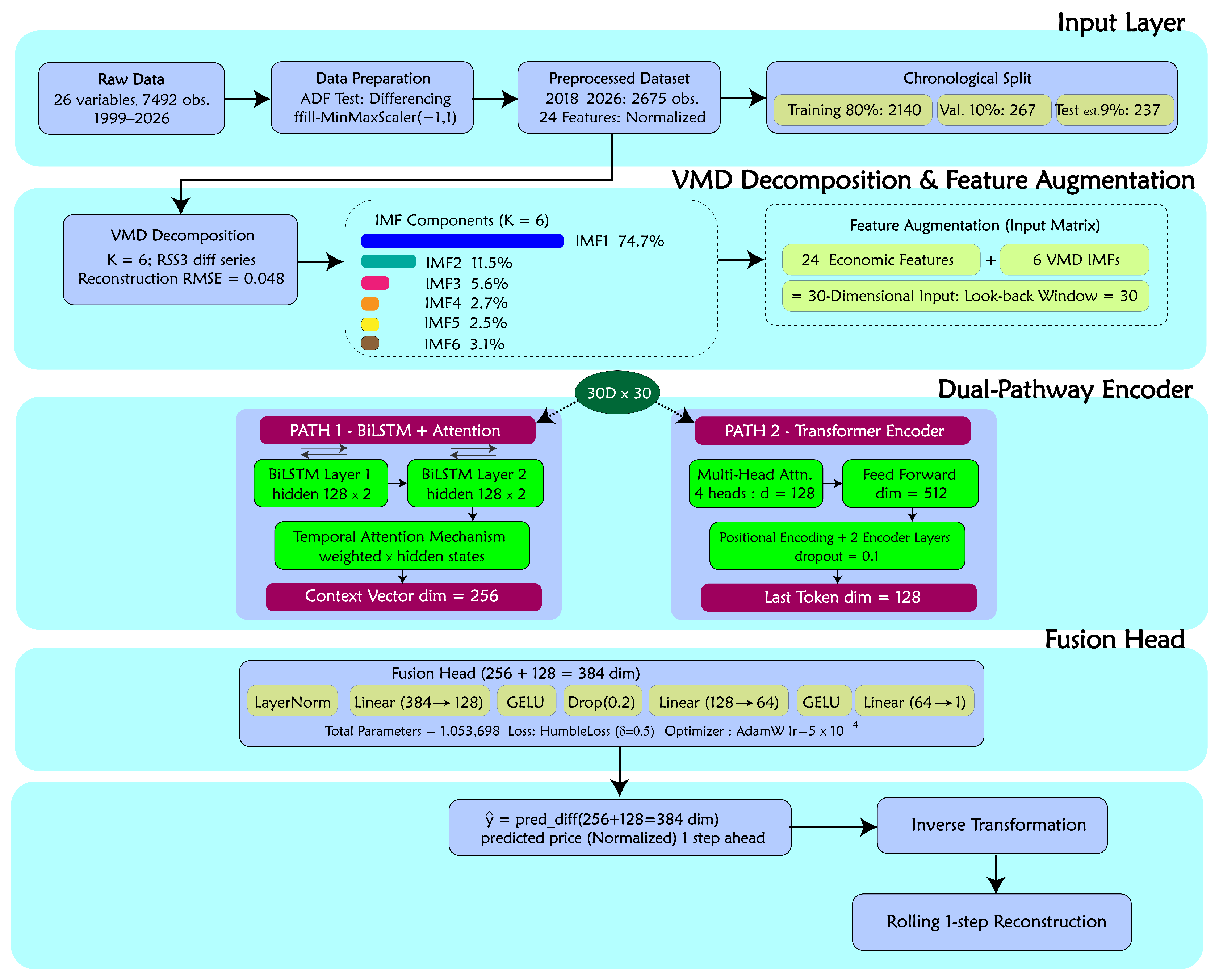
The proposed model uses a single primary encoder pathway: A two-layer Bidirectional LSTM with temporal attention, followed by a dense output head. Transformer-only and BiLSTM–Transformer variants are implemented only as ablation controls and are not part of the final primary model; Section 3.3 reports the ablation evidence motivating this choice. The complete primary architecture is summarised in

Table 5. Architecture summary—VMD-Augmented BiLSTM.

Component	Configuration	Output Dim	Notes
Input	30 features × 30 time steps	${\mathbb{R}}^{30\times 30}$	Primary and control
BiLSTM	Hidden = 128, 2 layers, bidirectional, dropout = 0.2	${\mathbb{R}}^{256/\mathit{step}}$	Primary encoder
Temporal Attention	Learnable scalar weights over $L=30$ steps	$\mathbf{c}\in {\mathbb{R}}^{256}$	Primary encoder
Input Projection	Linear($30\to 128$)	${\mathbb{R}}^{30\times 128}$	Ablation control only
Transformer Encoder	$d=128$, 4 heads, 2 layers, FFN = 512, dropout = 0.1	$z_L\in {\mathbb{R}}^{128}$	Ablation control only
Fusion Head	LN → Linear($384\to 128$) → GELU → Drop → Linear($64\to 1$)	$\Delta {\widehat{p}}_t\in \mathbb{R}$	Ablation control only
Total parameters	∼573,000 (primary BiLSTM only); 1,053,698 (full hybrid control)	—

; the control architecture is illustrated in Figure 3.

2.3.1. Primary Encoder: BiLSTM with Temporal Attention

A two-layer Bidirectional LSTM [58] with hidden size $H=128$ per direction processes the input sequence simultaneously in the forward and backward temporal directions. The bidirectional scope is strictly internal to the look-back window $[\tau -L+1,\tau ]$ defined relative to the forecast origin $\tau$: the backward pass propagates information from time $\tau$ back to time $\tau -L+1$, and the model never accesses observations from time $\tau +1$ or later when generating the forecast for $\Delta p_{\tau +1}$. This is structurally distinct from look-ahead leakage, in which a forecast at $\tau$ would use information from $\tau +1$ or later. The concatenated hidden state at each step $s\in [\tau -L+1,\tau ]$ within the look-back window is

$$h_s=\left[h_s^{\to };h_s^{\leftarrow }\right]\in {\mathbb{R}}^{2H}$$

(6)

where $h_s^{\to }$ and $h_s^{\leftarrow }$ are the forward and backward hidden states, respectively, and $H=128$, yielding a 256-dimensional representation. A learned temporal attention mechanism aggregates the L hidden states across the look-back window into a context vector:

$${\alpha }_s=\mathrm{softmax}\left(\tanh \left(W_a·h_s+b_a\right)\right)\in {\mathbb{R}}^L$$

(7)

$$c={\displaystyle \sum _{s=\tau -L+1}^{\tau }}{\alpha }_s·h_s\in {\mathbb{R}}^{2H}$$

(8)

where $W_a\in {\mathbb{R}}^{2H\times 1}$ and $b_a\in \mathbb{R}$ are learnable parameters. The context vector $c\in {\mathbb{R}}^{256}$ summarises the look-back window $[\tau -L+1,\tau ]$ with emphasis on the most informative time steps; the next-step forecast $\Delta {\widehat{p}}_{\tau +1}$ is computed from c via the output head described in Section 2.3.3.

2.3.2. Control Architecture for Ablation: Transformer Encoder Pathway

This pathway is evaluated only as an ablation control; the primary VMD-Augmented BiLSTM model omits it entirely. A two-layer Transformer encoder [35] operates on a linearly projected version of the input sequence. Each input token is first projected to a $d_{\mathrm{model}}=128$ dimensional space and augmented with a learnable positional embedding:

$$z_{\tau }=W_{\mathrm{proj}}·x_{\tau }+p_{\tau }\in {\mathbb{R}}^{d_{\mathrm{model}}}$$

(9)

where $x_{\tau }$ is the input feature vector, $W_{\mathrm{proj}}\in {\mathbb{R}}^{d_{\mathrm{model}}\times 30}$ is the projection matrix, $p_{\tau }\in {\mathbb{R}}^{d_{\mathrm{model}}}$ is the learnable positional encoding for position $\tau$, and $d_{\mathrm{model}}=128$. Learnable positional encodings are preferred over fixed sinusoidal encodings because financial time series exhibit irregular temporal patterns that may not conform to fixed periodic representations.

Each Transformer encoder layer applies multi-head self-attention followed by a positionwise feed-forward network with residual connections and layer normalisation:

$$\mathrm{Attention}(Q,K,V)=\mathrm{softmax}\left({\displaystyle \frac{Q{K}^{\top }}{\sqrt{d_k}}}\right)V$$

(10)

where Q, K, and V are the query, key, and value matrices derived from linear projections of the token embeddings, while $d_k$ is the dimension of the key vectors. The model uses $n_{\mathrm{heads}}=4$ attention heads, feed-forward dimension 512, and dropout rate 0.1. The final-step representation $z_L\in {\mathbb{R}}^{128}$ is taken as the Transformer pathway output in the ablation-control architecture.

2.3.3. Output Head (Primary Model) and Fusion Head (Ablation Control)

For the primary VMD-Augmented BiLSTM model, the attention-derived BiLSTM context vector $c\in {\mathbb{R}}^{256}$ is passed directly to a dense output head; no fusion is applied because the primary model uses only a single encoder pathway:

$$\Delta {\widehat{p}}_{\tau +1}=f_{\mathrm{out}}\left(c\right).$$

(11)

For the primary model, the output head is LayerNorm(256) → Linear($256\to 128$) → GELU → Dropout($p=0.2$) → Linear($128\to 64$) → GELU → Linear($64\to 1$). For the full BiLSTM–Transformer control architecture used only in the ablation analysis, the BiLSTM context vector and the Transformer last-token representation are first concatenated into a joint vector $v=[c;z_L]\in {\mathbb{R}}^{384}$, then passed through the fusion head: LayerNorm(384) → Linear($384\to 128$) → GELU → Dropout($p=0.2$) → Linear($128\to 64$) → GELU → Linear($64\to 1$). GELU activation is adopted because it provides smoother gradient flow than ReLU for regression tasks on continuous financial targets, consistent with its use in recent Transformer-based forecasting architectures [41,59,60,61].

The scalar output ${\widehat{y}}_{\tau +1}$ represents the predicted normalised price change $\Delta {\tilde{p}}_{\tau +1}$. The actual price change is recovered via inverse min–max transformation (Equation (3)), and the corresponding price level is reconstructed using a rolling one-step scheme: ${\widehat{p}}_{\tau +1}=p_{\tau }+\Delta {\widehat{p}}_{\tau +1}$.

2.4. Model Training

The model is trained end to end on the Stage 3 training partition ($n=2140$ observations, 2018–2023) using the configuration summarised in

Table 6. Training hyperparameters.

Hyperparameter	Value	Rationale
Loss function	Huber Loss ($\delta =0.5$)	Robust to outlier spikes
Optimiser	AdamW (LR $=5\times {10}^{-4}$, wd $={10}^{-4}$)	Adaptive LR + weight decay
LR scheduler	ReduceLROnPlateau ($\times 0.5$, patience 10)	Reduce on validation plateau
Early stopping	Patience $=30$ epochs	Prevent overfitting
Max epochs	300	Upper bound
Batch size	32	Mini-batch SGD
Look-back L	30 trading days	$\sim 6$ trading weeks of context
Total parameters	∼573,000 primary model; 1,053,698 full hybrid control

.

The Huber loss with threshold $\delta$ is defined as

$${\mathcal{L}}_{\delta }(y,\widehat{y})=\left\{\begin{array}{cc}{\displaystyle \frac{1}{2}}{(y-\widehat{y})}^2\hfill & \mathrm{if}|y-\widehat{y}| \le \delta \hfill \\ \delta \left(|y-\widehat{y}|-{\displaystyle \frac{1}{2}}\delta \right)\hfill & \mathrm{otherwise}\hfill \end{array}\right.$$

(12)

The choice of $\delta =0.5$ was determined by grid search over $\delta \in \{0.1,0.3,0.5,1.0\}$ on the validation set; $\delta =0.5$ provides quadratic sensitivity for small prediction errors while bounding the influence of large price shocks on gradient updates. The look-back window $L=30$ was selected to cover approximately six trading weeks, capturing both intra-month cyclical patterns and cross-market lag effects without introducing excessive computational cost; sensitivity to L is reported in Appendix F.

2.5. Evaluation Protocol, Baselines, and Multi-Step Extension

Model performance is assessed across two complementary evaluation spaces. Primary metrics are computed on the predicted and actual first-differenced series ($\Delta {\widehat{p}}_t$ vs. $\Delta p_t$) in real units of Baht/kg/day after inverse transformation (Equation (3)). These directly measure the model’s ability to predict daily price movements. Supplementary price-level metrics (MAE, RMSE, MAPE, and $R^2$) are computed on the reconstructed series ${\widehat{p}}_t=p_{t-1}+\Delta {\widehat{p}}_t$ and are reported for completeness only; their values are inflated by an autoregressive anchor effect and do not reflect additional predictive skill in the differenced space.

In

Table 7. Primary evaluation metrics—differenced series.

Metric	Formula	Interpretation
MAE	${\displaystyle \frac{1}{n}\sum \left|\Delta p_t-\Delta {\widehat{p}}_t\right|}$	Average magnitude error (Baht/kg/day)
RMSE	${\displaystyle \sqrt{\frac{1}{n}\sum {\left(\Delta p_t-\Delta {\widehat{p}}_t\right)}^2}}$	Penalises large errors
Pearson r	$\mathrm{corr}(\Delta p_t,\Delta {\widehat{p}}_t)$	Linear association strength
Directional Accuracy (DA)	${\displaystyle \frac{1}{n}\sum \mathbb{1}\left[\mathrm{sign}(\Delta {\widehat{p}}_t)=\mathrm{sign}(\Delta p_t)\right]}$	% of days with correct direction; n excludes days where $\Delta p_t=0$
StdR	$\mathrm{std}(\Delta \widehat{p})/\mathrm{std}(\Delta p)$	$=1$ ideal; <0.2 indicates variance collapse

Note: DA is computed directly on the differenced series—$\mathrm{sign}(\Delta {\widehat{p}}_t)$ vs. $\mathrm{sign}(\Delta p_t)$—not on the reconstructed price level. Days on which $\Delta p_t=0$ are excluded from the denominator ($n^{\ast }$). Following Zhu et al. [7], p. 6, DA $>0.6$ is regarded as the threshold for practically meaningful directional prediction.

, Pearson’s r and StdR are reported as co-primary metrics following the evaluation framework of Taylor [45] (pp. 7183–7184), who shows that neither metric is sufficient alone—high correlation does not guarantee correct amplitude, and low RMS error does not imply that forecast variance faithfully reproduces the target series—and in agreement with Mehdiyev et al. [62] (pp. 264–265) and Kyriakidis et al. [63] (pp. 104–105), who demonstrate that robust forecast evaluation requires concurrent consideration of multiple criteria because model rankings vary substantially across metrics.

DA is computed directly on the differenced series—$\mathrm{sign}(\Delta {\widehat{p}}_t)$ vs. $\mathrm{sign}(\Delta p_t)$—not on the reconstructed price level. Days on which $\Delta p_t=0$ are excluded from the denominator ($n^{\ast }$). Following Zhu et al. [7] (p. 6), DA $>0.6$ is regarded as the threshold for practically meaningful directional prediction. However, this threshold should be interpreted alongside confusion-matrix and variance-ratio diagnostics: Costantini et al. [49] show that raw DA becomes materially informative only when paired with magnitude-sensitive directional value measures, and Rajpal et al. [43] (pp. 13–15) demonstrate that symmetric loss objectives can produce apparently acceptable DA through one-sided prediction that is fully revealed only by specificity and StdR diagnostics.

The use of a ratio-based dispersion metric as a collapse diagnostic is consistent with the Variability Collapse Index proposed by Xu and Liu [64], who derive a formally analogous quantity from the minimum MSE linear probing loss and demonstrate that ratio-based metrics are invariant to invertible linear transformations of the feature space—a property that point-estimate collapse measures such as within-class distance do not possess. Four baseline models are evaluated on the identical test partition ($n=175$ observations after deduplication, 18 September 2025–27 February 2026) using the same protocol; their specifications are summarised in

Table 8. Baseline model specifications.

Baseline	Specification	Purpose
Naive No-Change	$\Delta {\widehat{p}}_t=0\forall t$	Lower bound; tests if any model beats zero-change forecast
Naive Random Walk	$\Delta {\widehat{p}}_t=\Delta p_{t-1}$	Standard persistence baseline for differenced series
ARIMA(2,0,2)	AIC-selected via grid search on training set; rolling 1-step refitting on test set	Linear time-series benchmark *
Vanilla LSTM	Unidirectional 2-layer LSTM (hidden $=128$); same 24 economic features as input; no VMD stage	Ablates the VMD-as-features contribution

Notes: * ARIMA serves as the natural linear benchmark because it dominates the early rubber forecasting literature—Ref. [12] identifies ARIMA(1,1,0) as the best-fitting model for Malaysian SMR20, and Ref. [13] uses ARIMA as the univariate baseline against which structural supply–demand models are evaluated—making it the standard against which forecasting advances for this commodity are measured.

.

• Multi-Step Forecasting Extension.

In addition to the one-step-ahead horizon ($h=1$), this study evaluates the proposed model under a direct multi-step forecasting strategy for horizons $h\in \{1,2,3,5,10,20,30\}$ trading days. This study adopts the direct forecasting strategy, training a separate model for each horizon h to avoid recursive error accumulation. While this requires H independent models, the approach avoids recursive error propagation and provides horizon-specific forecasts [65]. Under the direct strategy, the training target is shifted accordingly:

$$y_i^{\left(h\right)}=\Delta p_{i+L+h-1},h=1,2,\dots ,H$$

(13)

where $y_i^{\left(h\right)}$ denotes the target value for the h-step-ahead forecast associated with sample i, defined as the realized price change $\Delta p_{i+L+h-1}$ at forecast horizon h.

The emphasis on short lead times is consistent with prior VMD-based forecasting studies, where predictive gains from decomposition are strongest at near-term horizons and tend to weaken as the forecast horizon extends [66]. For $h>1$, future exogenous features are unavailable at prediction time; the model receives only the values observed within the look-back window and makes no use of forward-looking information. This is equivalent to assuming that all exogenous conditions remain constant beyond the last observation, a limitation discussed in Section 4.

3. Results

This section reports the empirical results of the proposed VMD-Augmented BiLSTM framework. All primary evaluations are conducted on the Stage 3 out-of-sample test set ($n=175$ effective observations after deduplication, 18 September 2025–27 February 2026). Section 3.1 outlines the evaluation framework; Section 3.2 presents the VMD signal decomposition; Section 3.3 reports the ablation analysis confirming the contribution of each architectural component; Section 3.4 reports out-of-sample forecast performance against benchmark models; Section 3.5 presents directional bias diagnostics; and Section 3.6 reports multi-step forecast skill across horizons $h\in \{1,2,3,5,10,20,30\}$.

3.1. Evaluation Framework

The primary evaluation is conducted in differenced space using five metrics. Directional Accuracy (DA) measures the proportion of days on which the predicted sign of the price change matches the realised sign; days on which $\Delta p_t=0$ are excluded from the denominator. Pearson correlation (r) quantifies the linear association between predicted and actual price changes. MAE and RMSE measure average and root-mean-squared prediction error in Baht/kg/day. The Standard Deviation Ratio (StdR) is defined as

$$\mathrm{StdR}={\displaystyle \frac{\mathrm{std}(\Delta \widehat{p})}{\mathrm{std}(\Delta p)}}$$

(14)

StdR equals 1.0 under ideal forecast dispersion and approaches 0 when a model produces near-constant predictions regardless of actual variation. A value below 0.20 is taken as evidence of variance collapse—a failure mode in which a model learns the unconditional mean rather than the conditional distribution of price changes. This convergence toward the unconditional mean is a forecast-output underdispersion phenomenon, conceptually parallel to the broader distributional-concentration failures discussed in the multi-stage estimation literature [42] (pp. 755–757), and directly analogous to the one-sided prediction regimes identified by Rajpal et al. [43] (pp. 13–15), in which symmetric loss objectives produce degenerate directional outputs whose apparent performance masks near-zero predictive content. Rajpal et al. [43] further show that this degenerate regime produces severe imbalance between recall and specificity—a pathology that high DA alone cannot detect, reinforcing the need for confusion-matrix and variance-ratio diagnostics alongside directional hit-rate statistics. StdR is the most important diagnostic for differenced commodity price models because high DA can be achieved trivially by predicting the majority class, whereas reproducing the variance of the target series requires predictive information beyond the unconditional sign distribution.

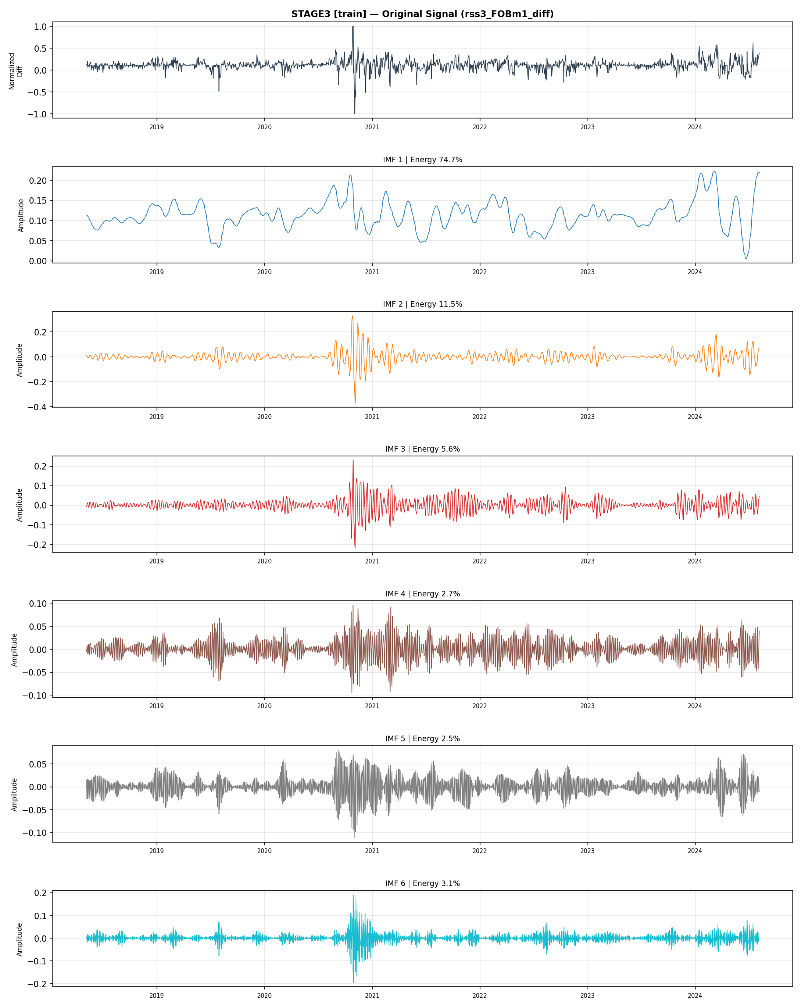
Price-level metrics—specifically $R^2$ and MAPE—are included in Section 3.4 for completeness only. These statistics are inflated by the autoregressive anchor effect: because the reconstructed level ${\widehat{p}}_t=p_{t-1}+\Delta {\widehat{p}}_t$ inherits the previous day’s price regardless of forecast quality, $R^2$ and MAPE at the level will appear favourable even when the differenced-space forecast is uninformative. They therefore carry no additional diagnostic value beyond the five primary metrics reported in Table 7. The VMD decomposition of the Stage 3 differenced price series, obtained under the expanding-window procedure with $K=6$, is shown in Figure 4.

3.2. VMD of the RSS3 Price Series

Variational Mode Decomposition was applied to the differenced RSS3 FOBm1 series ($\Delta p_t$) over the Stage 3 training and validation partitions ($n=2407$ observations). The decomposition with $K=6$ modes (see Appendix C) achieved a reconstruction RMSE of 0.048 normalised units, representing 3.2% of the series standard deviation, confirming that the six components collectively reconstruct the original differenced series with minimal residual error.

IMF₁ accounts for 74.7% of total signal energy and exhibits the lowest centre frequency ($f\approx 0.0005$), consistent with the long-run structural trends documented in the literature on natural rubber, including fluctuations in global automobile production and plantation supply cycles [7]. The two intermediate-frequency components (IMF₂–IMF₃) collectively capture 17.1% of energy and correspond to temporal scales of one to four weeks, consistent with the inventory adjustment cycles and seasonal tapping rhythms documented in rubber export data from Thailand, Indonesia, and Malaysia [7,30]. The structural dominance of IMF₁ is further consistent with the simultaneous supply–demand framework of Arunwarakorn et al. [50] (pp. 8–9), who show that equilibrium rubber prices are anchored by slow-moving fundamentals—plantation area, synthetic rubber prices, GDP growth, and crude oil—operating over multi-year cycles rather than at the weekly or daily frequencies captured by IMF₂–IMF₆. The mid- to high-frequency residuals (IMF₄–IMF₆) account for 8.3% of energy and reflect intra-day speculative activity and short-term information shocks operating at sub-weekly scales. Full VMD decomposition results, including centre frequencies and energy shares for each mode, are summarised in

Table 9. VMD results—Stage 3, $K=6$ (expanding window).

IMF	Label	Centre Freq.	Energy (%)	Economic Interpretation
1	Trend	$f\approx 0.0005$	74.7%	Long-run structural price trend (macroeconomic cycle, supply shifts)
2	Low-freq.	$f\approx 0.072$	11.5%	Weekly–monthly market cycles (export dynamics, inventory)
3	Low-freq.	$f\approx 0.120$	5.6%	Bi-weekly fluctuations (tapping seasons, policy announcements)
4	Mid-freq.	$f\approx 0.236$	2.7%	Short-term trading noise (intra-day, speculative positions)
5	High-freq.	$f\approx 0.332$	2.5%	Short-horizon information shocks
6	High-freq.	$f\approx 0.429$	3.1%	High-frequency microstructure noise
Total		Reconstruction RMSE $=0.048$		Near-perfect reconstruction

.

The top panel shows the original $\Delta p_t$, while the remaining panels present IMF₁–IMF₆ with their centre frequencies and energy shares. IMF₁ dominates the signal (74.7% energy), capturing the low-frequency trend, whereas IMF₄–IMF₆ mainly represent mid- to high-frequency noise.

3.3. Ablation Study

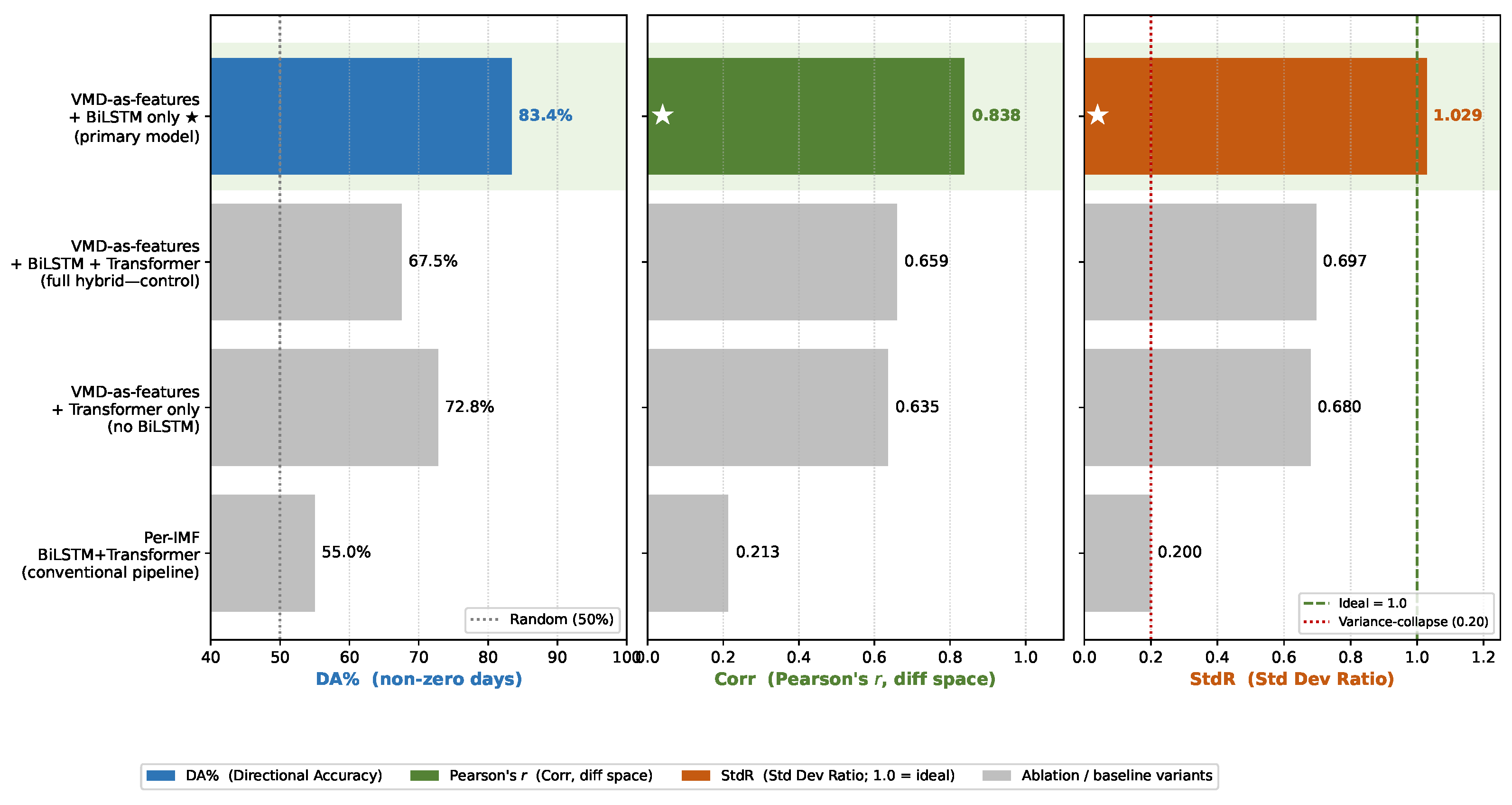
To verify the contribution of each architectural component, an ablation analysis was conducted on the deduplicated, leakage-free Stage 3 test partition ($n=175$). Four configurations were compared: (i) the full VMD-Augmented BiLSTM–Transformer hybrid control, (ii) the BiLSTM-only model (Transformer pathway removed), (iii) the Transformer-only model (BiLSTM encoder removed), and (iv) the conventional per-IMF decomposition–forecast pipeline. The results are summarised in

Table 10. Ablation study results—test set ($n=175$, seed 42). ★ marks the primary configuration.

Model Variant	DA%	Corr	StdR	Key Finding
Per-IMF BiLSTM+Transformer (conventional VMD pipeline)	$55.0\%$	$0.213$	$0.200$	Variance collapse on differenced series
VMD-as-features + BiLSTM only ★ (primary model)	$83.4\%$	$0.838$	$1.029$	Multi-seed: $r=0.821\pm 0.016$
VMD-as-features + Transformer only (no BiLSTM)	$72.8\%$	$0.635$	$0.680$	Self-attention alone captures less
VMD-as-features + BiLSTM + Transformer (full hybrid—control)	$67.5\%$	$0.659$	$0.697$	Transformer adds parameters but no gain

.

The ablation results identify the bidirectional LSTM pathway as the principal architectural driver of accuracy. The BiLSTM-only variant achieves Pearson’s $r=0.838$, StdR = 1.029, and DA = 83.4%—matching or exceeding the performance of the full hybrid across all primary metrics at seed 42. The Transformer-only variant attains lower correlation ($r=0.635$) and comparable variance dispersion (StdR = 0.680), indicating that self-attention alone does not capture multi-scale temporal structure as effectively as bidirectional recurrence does. The full hybrid configuration ($r=0.659$, StdR = 0.697 at seed 42) does not improve upon BiLSTM-only in this setting.

Multi-seed sensitivity analysis ($n=5$ seeds: 42, 123, 2024, 7, 999) confirms this pattern: BiLSTM-only attains $r=0.821\pm 0.016$ versus the full hybrid’s $0.651\pm 0.054$, with no overlap between the two per-seed distributions of Pearson correlation. The BiLSTM-only configuration is therefore adopted as the primary model and reported as VMD-Augmented BiLSTM in subsequent sections.

The per-IMF conventional pipeline shows the largest performance gap. Five separate models, each forecasting one IMF and summed at inference time, attain $r=0.213$ with StdR = 0.200—at the variance-collapse threshold, where forecasts become nearly constant in dispersion. This finding directly motivates the VMD-as-features design adopted throughout this study: by exposing all IMFs jointly to a single forward pass, the encoder learns cross-scale interactions that the additive ensemble cannot recover. This empirical pattern—in which forecast variance shrinks when finite-sample approximation error compounds across successive estimation stages—is conceptually parallel to the underdispersion outcomes discussed in the literature on multi-stage estimation [42] (p. 757), though the present result is established here as an empirical finding on differenced commodity-price forecasts rather than derived from a theorem.

The ablation patterns shown in Figure 5 support three observations. The BiLSTM-only configuration achieves the strongest balance across the three primary metrics. The full hybrid (BiLSTM + Transformer) adds 84% more parameters without improving any of the three metrics, indicating that the Transformer pathway is redundant when VMD features are already provided. The Transformer-only variant captures less correlation than the BiLSTM-only variant, indicating that bidirectional recurrence is the principal predictive driver. The per-IMF conventional pipeline exhibits variance collapse (StdR $=0.200$), motivating the VMD-as-features design adopted in the proposed framework.

3.4. Out-of-Sample Forecast Performance

Now that the contribution of each component has been confirmed through ablation, this section evaluates the proposed VMD-Augmented BiLSTM model against four external benchmarks on the deduplicated, leakage-free test partition ($n=175$).

The Naive No-Change model ($\Delta {\widehat{p}}_t=0$) serves as a lower bound; any useful forecasting model must exceed it in directional accuracy. The Naive Random Walk ($\Delta {\widehat{p}}_t=\Delta p_{t-1}$) tests whether recent momentum has predictive value. ARIMA(2,0,2), selected by AIC grid search, represents the linear time-series benchmark. Vanilla LSTM (unidirectional, two-layer, same 24 economic features as input, no VMD) provides an additional ablation of the VMD-as-features contribution against a standard deep learning baseline.

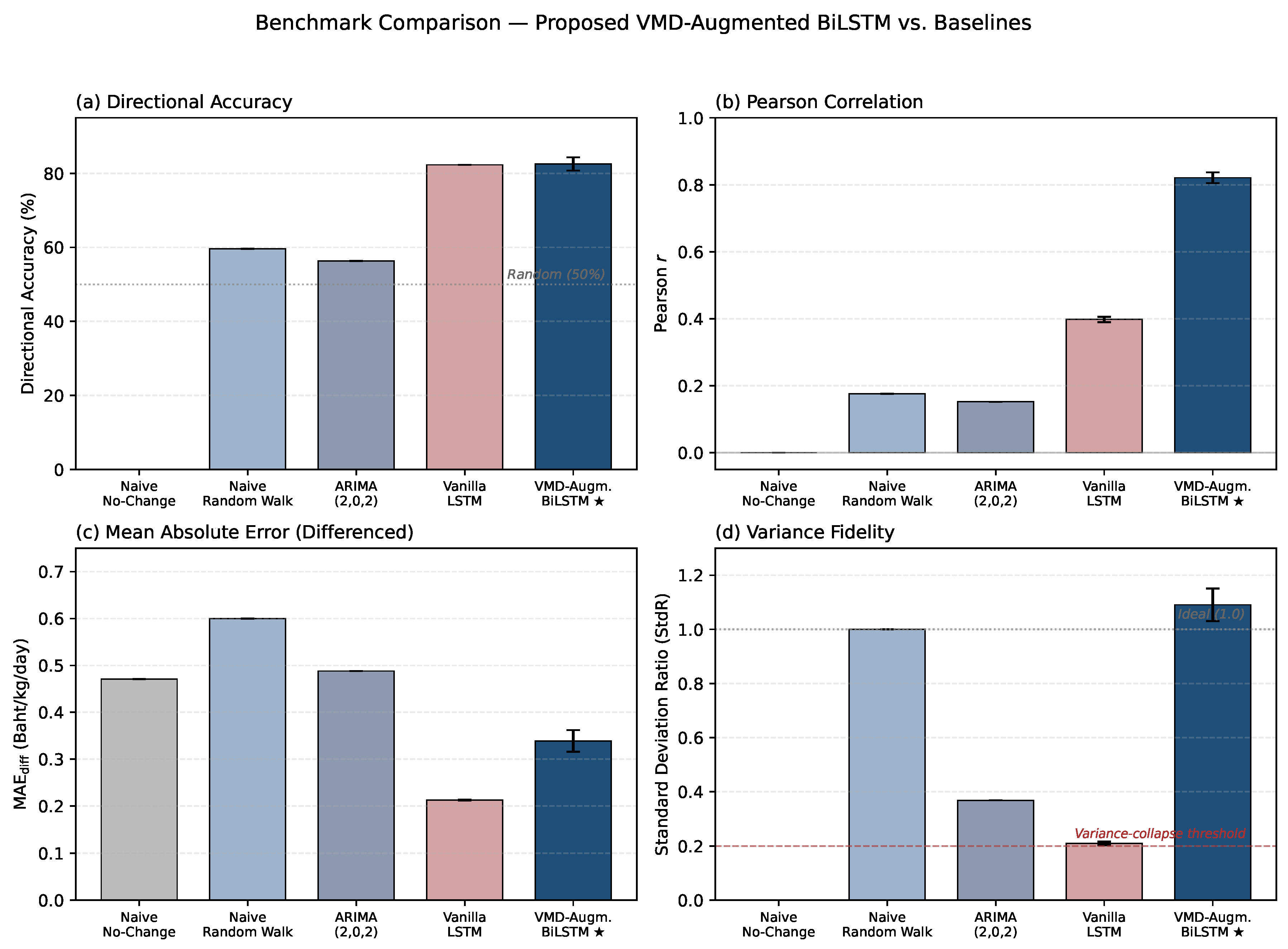
The proposed VMD-Augmented BiLSTM achieves the strongest balance across primary metrics on the deduplicated leakage-free test partition. Across five random seeds, the model attains Pearson’s $r=0.821\pm 0.016$ and StdR $=1.091\pm 0.060$, improving correlation by approximately $+0.67$ over ARIMA(2,0,2). Crucially, the variance ratio (StdR ≈ 1.09) sits close to unity, indicating that predicted amplitudes are well calibrated to the realised magnitude distribution—a property that neither ARIMA (StdR = 0.368) nor Vanilla LSTM (StdR = $0.210\pm 0.007$) achieves. The Vanilla LSTM result is particularly informative: despite attaining directional accuracy statistically indistinguishable from the proposed model ($82.29\%\pm 0.00$ vs. $82.52\%\pm 1.79$), its predictions exhibit pronounced variance collapse, with predicted dispersion at only one-fifth that of the realised series. The Vanilla LSTM attains lower MAE and RMSE than the proposed model precisely because its forecasts are variance-collapsed toward the conditional mean: when the predicted series has near-zero dispersion, the squared and absolute deviations from the realised series shrink mechanically, mimicking apparent accuracy without producing usable directional or magnitude information. Lower error alone is therefore not evidence of superior forecast usefulness; the joint diagnostic $(r,\mathrm{StdR})$ must accompany level metrics for a faithful assessment of forecast skill. The mechanisms generating this divergence are analysed in Section 3.5.

This margin is consistent with the broader rubber forecasting literature showing that purely univariate linear models are structurally insufficient once commodity-specific drivers are made explicit: Khin and Thambiah [13] demonstrate that a simultaneous supply–demand system outperforms ARIMA across all accuracy criteria, while Eng and Khalid [26] confirm that LSTM dominates ARIMA on Malaysian SMR20—establishing that the gain over ARIMA reported here reflects a systematic pattern rather than a sample-specific outcome. The directional accuracy of 82.5% ± 1.8% (across five seeds) substantially exceeds that of the random baseline (50%) on the deduplicated test partition, consistent with the predictive content carried by the 24 economic features and the VMD-augmented frequency components.

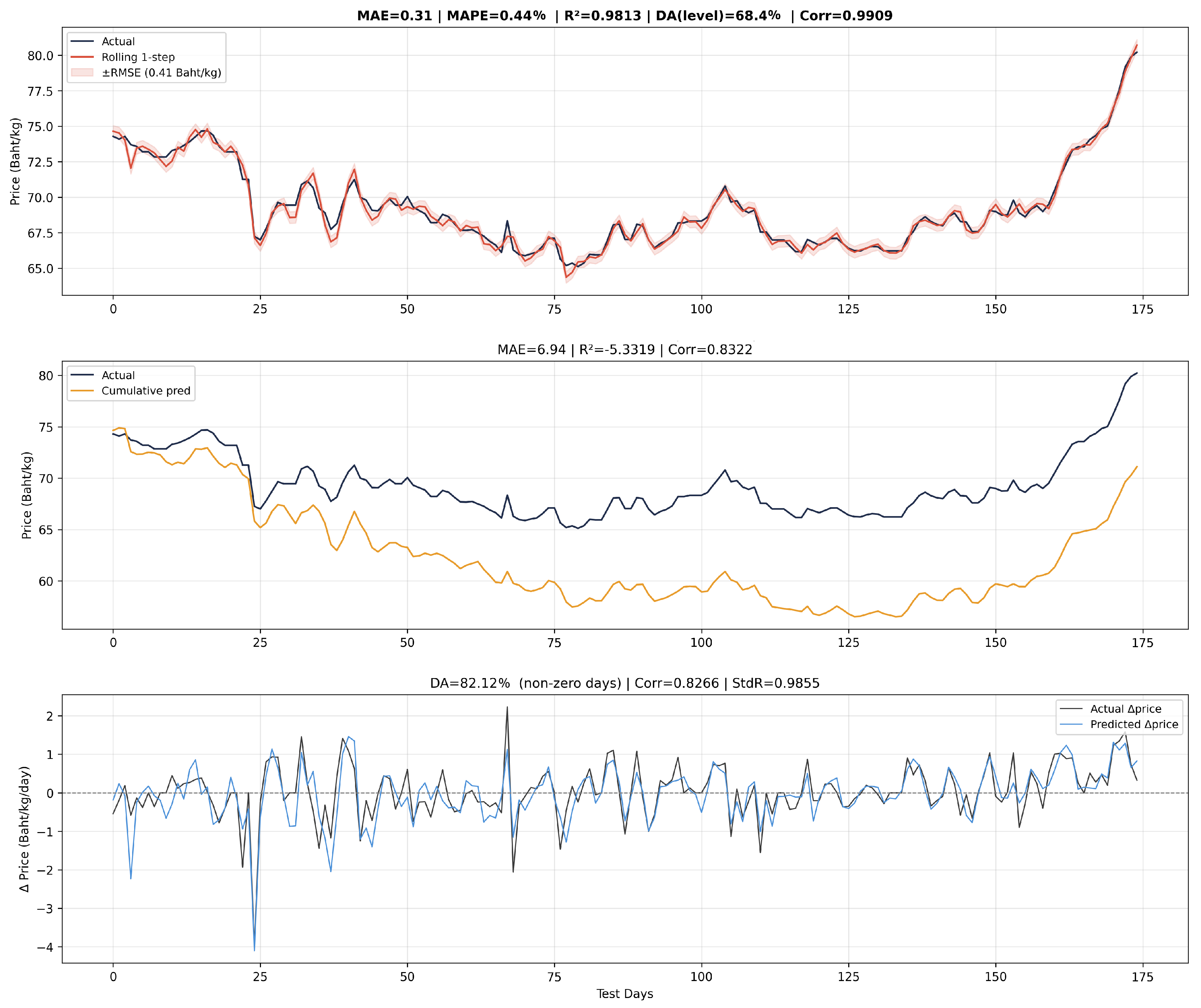
The model’s predictive skill is consistent with the layered cross-market structure documented by Kepulaje et al. [9] (pp. 159–161) and Pinitjitsamut [52]: because SHFE signals are incorporated into FOB Bangkok with a lag and pass-through remains incomplete and asymmetric in the short run, one-day-ahead predictability beyond the autoregressive baseline is structurally limited—making a Pearson correlation of $0.821\pm 0.016$ across five random seeds on the differenced series a substantively strong result rather than an expected one. The VMD-Augmented BiLSTM successfully tracks the realised RSS3 price trajectory across the test period, capturing both directional movements and amplitude variation (Figure 6).

The figure presents three views of the seed-42 test realisation. The top panel shows the rolling one-step price-level reconstruction, ${\widehat{p}}_t=p_{t-1}+\Delta {\widehat{p}}_t$, against the realised level series; the close fit reflects the autoregressive anchor effect (Section 3.1) rather than underlying differenced-space skill. The middle panel makes this transparent: the cumulative-prediction path—predicted increments accumulated without re-anchoring—drifts substantially over the test window, demonstrating why performance must be assessed in the differenced space. The bottom panel reports the daily first-differenced predictions $\Delta {\widehat{p}}_t$ versus realised $\Delta p_t$ (Baht/kg/day)—the primary evaluation space—with predictions tracking actuals in both sign and amplitude, consistent with the multi-seed StdR of $1.091\pm 0.060$ in

Table 11. Out-of-sample forecasting performance—test set ($n=175$, deduplicated, leakage-free). ★ marks the primary model.

Model	Differenced Space (Primary)					Price Level (Supplementary)
	DA%	Corr	${\mathbf{MAE}}_{\mathit{d}}$	${\mathbf{RMSE}}_{\mathit{d}}$	StdR	${\mathbf{MAE}}_{\mathit{p}}$	${\mathbf{RMSE}}_{\mathit{p}}$	MAPE%
Naive No-Change	$0.0\%$	$0.000$	$0.471$	$0.698$	$0.000$	$0.471$	$0.698$	$0.68\%$
Naive Random Walk	$59.6\%$	$0.176$	$0.600$	$0.895$	$1.000$	$0.600$	$0.895$	$0.87\%$
ARIMA(2,0,2)	$56.3\%$	$0.152$	$0.488$	$0.706$	$0.368$	$0.488$	$0.706$	$0.71\%$
Vanilla LSTM	$82.29\pm 0.00\%$	$0.398\pm 0.008$	$0.213\pm 0.001$	$0.295\pm 0.001$	$0.210\pm 0.007$	$0.213$	$0.295$	$0.31\%$
VMD-Augmented BiLSTM ★	$82.5\pm 1.8\%$	$0.821\pm 0.016$	$0.339\pm 0.023$	$0.456\pm 0.035$	$1.091\pm 0.060$	$0.339$	$0.456$	$0.49\%$
(mean ± SD over 5 seeds $\{7,42,123,999,2024\}$)

Notes: ${\mathrm{MAE}}_d$ and ${\mathrm{RMSE}}_d$ in Baht/kg/day. Price-level metrics (${\mathrm{MAE}}_p$, ${\mathrm{RMSE}}_p$, MAPE%) reported for comparability with the prior literature only; see Section 3.1 for discussion of the autoregressive anchor effect. ★ marks the primary model. Vanilla LSTM is reported as multi-seed (mean ± 1 SD across 5 seeds $\{7,42,123,999,2024\}$) following the same protocol as the proposed model, providing a directly comparable robustness baseline; the variance-collapse pattern of Vanilla LSTM is analysed in Section 3.5.

.

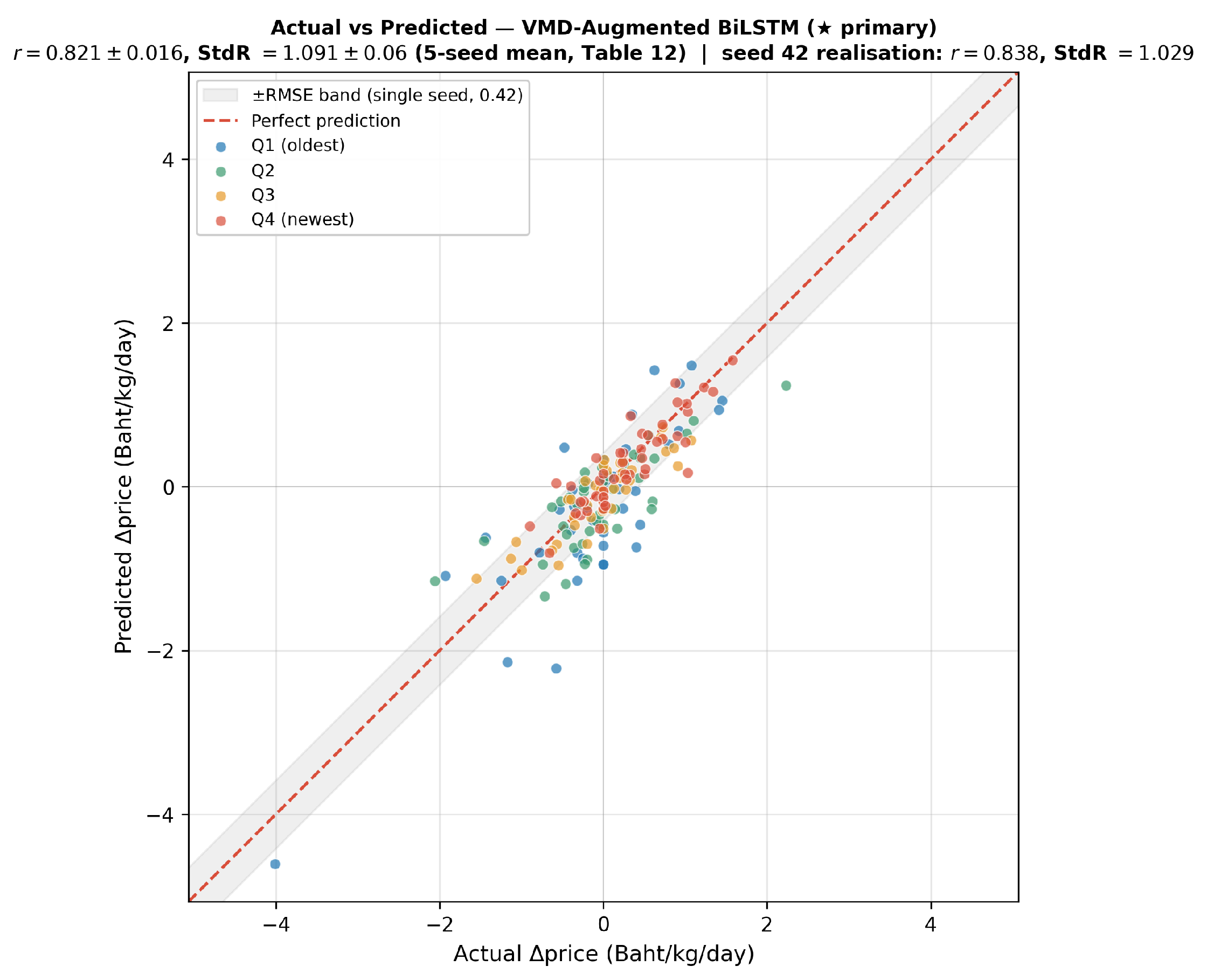
The StdR of 1.091 (mean across five seeds) is the highest StdR across all evaluated models and sits close to the ideal value of 1.0, indicating that the VMD-Augmented BiLSTM produces forecasts whose dispersion is well calibrated to the actual first-differenced series (Figure 7). By contrast, ARIMA (StdR = 0.368) substantially underdisperses, while Vanilla LSTM (StdR = $0.210\pm 0.007$ across five seeds) exhibits variance collapse at the diagnostic threshold of 0.20 introduced in Section 3.1—a regime in which the model has converged to near-flat forecasts that reproduce the empirical sign distribution of the test set without preserving its magnitude. This combination of high Pearson correlation, near-unity StdR, and 175-observation reproducibility across five seeds provides the strongest evidence in this study of forecasts whose dispersion and co-movement structure are jointly consistent with the realised series, rather than artefacts of mean reversion or sign-dominant predictions.

The price-level metrics reported in Table 11 should be interpreted with caution. The Naive No-Change model, which predicts zero price change on every day, achieves low level-space error despite having zero predictive content (DA $=0\%$, Corr $=0.000$). This confirms that price-level metrics alone cannot distinguish informative forecasts from a trivial baseline, as discussed in Section 3.1.

This is precisely the evaluation failure described by Taylor [45] (pp. 7183–7184): A forecast can appear numerically accurate while being dynamically wrong if it suppresses variance rather than tracking the stochastic structure of the series. Ampountolas [67] (pp. 2, 14–18) illustrates the same gap in commodity forecasting practice—standard MAE, MSE, and RMSE comparisons identify the model with smallest average error but cannot reveal whether the winning model reproduces distributional scale, making StdR and Pearson’s r indispensable complements rather than optional additions.

3.5. Directional Bias Analysis

Now that the VMD-Augmented BiLSTM has been established to achieve the best balance between correlation and variance fidelity, this section examines whether high directional accuracy in baseline models reflects predictive content beyond the unconditional sign distribution or merely reflects distributional bias. The analysis combines class-conditional recall with the variance-fidelity diagnostic on the $n=175$ test set (deduplicated) in

Table 12. Class-conditional recall summary—test set ($n=175$, deduplicated). Vanilla LSTM is reported under the multi-seed protocol (see subsequent analysis) to avoid the seed-dependent variation that single-run summaries would mask.

Model	Up Recall (%)	Down Recall (%)	DA (%)	StdR
Naive No-Change	0.0	0.0	0.0	0.000
ARIMA(2,0,2)	61.5	50.7	56.3	0.368
VMD-Augmented BiLSTM ★	82.1	84.9	$83.4★$	$1.029★$

Notes: ★ marks the proposed VMD-Augmented BiLSTM model and its best-in-column values for DA and StdR. Up recall = TP/(TP+FN), the proportion of actual up days correctly predicted. Down recall = TN/(TN + FP), the proportion of actual down days correctly predicted. DA computed on non-zero actual days only. Actual up days $=78$ (51.7%); actual down days $=73$ (48.3%). For VMD-Augmented BiLSTM, single-seed results shown (seed 42); multi-seed mean DA $=82.5\%\pm 1.8\%$ with down recall $=78.1\%\pm 5.5\%$ across 5 seeds (Table 11). Full $2\times 2$ confusion matrices, including FP and FN counts, are presented in the subsequent confusion-matrix analysis.

; full confusion matrices for visual inspection are presented in Figure 8.

The deduplicated test set contains 78 up days and 73 down days (non-zero observations), close to balanced—in contrast to the unbalanced 191 vs. 46 split that arose when SGX multi-contract records double-counted up days in the pre-deduplication version. The Naive Random Walk baseline attains DA = 59.6% by following the previous day’s direction with no recall asymmetry; ARIMA(2,0,2) attains DA = 56.3% with up recall 61.5% and down recall 50.7%, the latter being at the random-baseline threshold. The Vanilla LSTM baseline is reported separately under the multi-seed protocol in

Table 13. Vanilla LSTM multi-seed evaluation—test set ($n=175$, seeds $\{7,42,123,999,2024\}$). The proposed VMD-Augmented BiLSTM row is reproduced from Table 11 for direct comparison.

Model	DA%	Pearson’s r	StdR	MAEd	RMSEd
Vanilla LSTM	$82.29\pm 0.00$	$0.398\pm 0.008$	$0.210\pm 0.007$	$0.213\pm 0.001$	$0.295\pm 0.001$
VMD-Augmented BiLSTM ★	$82.52\pm 1.79$	$0.821\pm 0.016$	$1.091\pm 0.060$	$0.339\pm 0.023$	$0.456\pm 0.035$

Notes: ★ marks the proposed VMD-Augmented BiLSTM model. All values are reported as the mean ± 1 standard deviation across 5 random seeds. MAE_d and RMSE_d in Baht/kg/day on the differenced series. Vanilla LSTM architecture per Appendix D (single-directional, hidden $=128$, layers $=2$, dropout $=0.20$, no VMD modes). The pairing of $82.29\%$ directional accuracy with $r=0.398$ and StdR $=0.210$ illustrates the variance-collapse pathology discussed in the main text: high DA is achieved without magnitude fidelity, a regime that the DA-only criterion cannot detect.

, where its variance-collapse pattern is documented and analysed.

The VMD-Augmented BiLSTM (mean across seeds) attains DA $=82.5\%\pm 1.8\%$ with down recall $=78.1\%\pm 5.5\%$, indicating that its high directional accuracy reflects balanced sign tracking across both up and down days rather than a positive-bias artefact. Combined with the near-unity StdR, this confirms that the proposed model identifies directional turning points without sacrificing amplitude fidelity (Figure 9). Collectively, the confusion matrix diagnostics (Figure 8) and StdR comparison show that high directional accuracy must be interpreted jointly with variance fidelity and class-specific recall. This finding corroborates the work of Bürgi [46] (pp. 7909–7912), who demonstrates that DA is not a self-sufficient evaluation concept without knowledge of magnitude sensitivity and class composition, and McCarthy and Snudden [47] (pp. 1–7), who show that success ratios can exceed 0.5 mechanically under class imbalance. Costantini et al. [49] further show that DA becomes materially informative only when paired with magnitude-sensitive directional value measures that weight correct sign calls by the size of the realised move rather than treating all correct predictions as equivalent.

• Vanilla LSTM multi-seed evidence.

A direct empirical illustration of this pathology is obtained by re-evaluating the Vanilla LSTM baseline under the same five-seed protocol applied to the primary model. Across seeds $\{7,42,123,999,2024\}$, the architecture—single-directional LSTM with hidden dimension 128, two layers, and dropout 0.20, receiving the 24 economic features without the VMD modes—attains directional accuracy of $82.29\%\pm 0.00$, Pearson correlation $r=0.398\pm 0.008$, and StdR $=0.210\pm 0.007$ (Table 13). The zero standard deviation of DA across five independently initialised runs, in combination with the near-identical Pearson r and StdR values, indicates that the model has converged in every run to a forecast whose dispersion is sufficient only to identify the empirical sign distribution of the test sample, not to reproduce the magnitude of realised price changes. The variance ratio of $0.210$ sits at the diagnostic threshold of $0.20$ introduced in Section 3.1 and is consistent with the forecast-output underdispersion regime that motivates the variance-collapse diagnostic in this study, paralleling the broader literature on distributional-concentration failures in underdetermined estimation [42] (p. 757). By contrast, the proposed VMD-Augmented BiLSTM attains $r=0.821\pm 0.016$ and StdR $=1.091\pm 0.060$ on the same test partition, doubling the Pearson correlation and recovering near-ideal variance fidelity at a statistically indistinguishable directional accuracy ($82.52\%\pm 1.79$ vs. $82.29\%\pm 0.00$; difference within one standard deviation of the proposed model). This pairing of metrics provides the empirical anchor for the methodological argument advanced throughout this section: A model that achieves $82.29\%$ directional accuracy with $r=0.398$ and StdR $=0.210$ cannot be distinguished from a magnitude-preserving forecast on the DA criterion alone but is unambiguously identified as variance-collapsed under the joint $(r,\mathrm{StdR})$ diagnostic. The implication generalises beyond the present sample: Any reporting practice that relies on directional accuracy without complementary variance and correlation diagnostics will systematically fail to detect this class of degenerate forecast, which can otherwise pass as a competitive deep learning baseline.

3.6. Multi-Step Forecast Skill Degradation

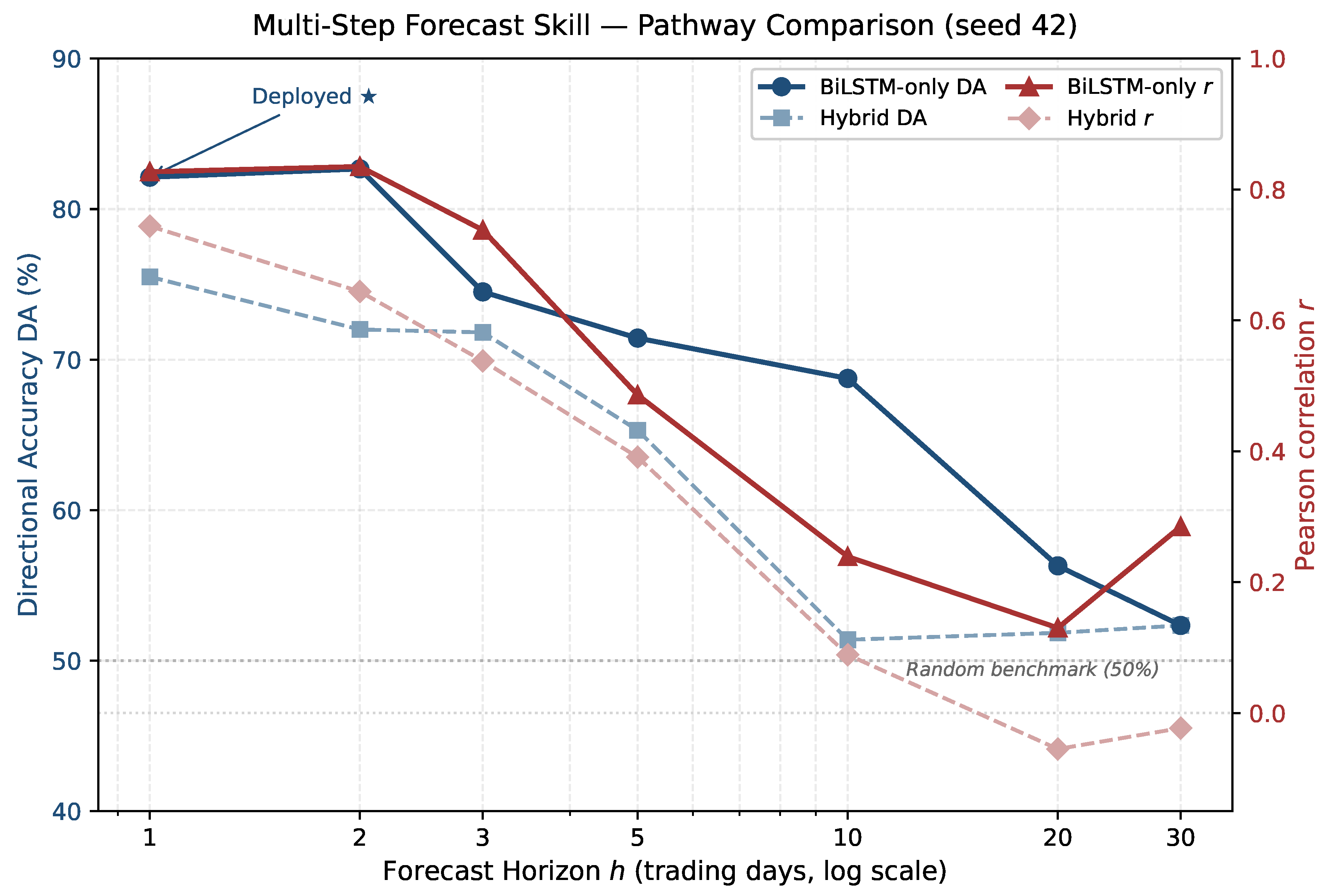
Forecast skill degradation across horizons is assessed using the direct multi-step strategy: A separate model is trained for each target horizon $h\in \{1,2,3,5,10,20,30\}$, with all other architecture and hyperparameter settings held constant. Both the dual-pathway BiLSTM–Transformer hybrid and the BiLSTM-only deployed configuration were trained side by side under the same data pipeline as Table 11 (seed 42), enabling a direct apples-to-apples comparison of how each architecture’s skill degrades as the horizon is extended. The full results are reported in

Table 14. Multi-step direct forecast performance—dual-pathway hybrid vs. BiLSTM-only configurations (seed 42, single-run, apples-to-apples). At $h=1$, the BiLSTM-only model attains $r=0.827$, consistent with the multi-seed Pearson correlation of $0.821\pm 0.016$ reported in Table 11.

Architecture	h	DA%	Pearson’s r	MAE (Bt/kg/d)	RMSE	StdR
Dual-pathway hybrid	1	75.5%	0.744	0.346	0.469	0.667
	2	72.0%	0.644	0.386	0.537	0.661
	3	71.8%	0.538	0.439	0.593	0.613
	5	65.3%	0.391	0.476	0.671	0.644
	10	51.4%	0.089	0.508	0.722	0.271
	20	51.9%	−0.055	0.498	0.729	0.025
	30	52.3%	−0.023	0.475	0.640	0.026
BiLSTM-only ★ (deployed)	1 ★	82.1%	0.827	0.309	0.411	0.985
	2	82.7%	0.835	0.281	0.385	0.827
	3	74.5%	0.738	0.347	0.479	0.682
	5	71.4%	0.486	0.416	0.616	0.475
	10	68.8%	0.239	0.468	0.691	0.265
	20	56.3%	0.130	0.495	0.722	0.126
	30	52.3%	0.285	0.466	0.639	0.007

Notes: ★ marks the proposed (deployed) BiLSTM-only configuration; the inner ★ at $h=1$ further identifies the primary forecast horizon reported throughout the main analysis. Bold values mark the dominant configuration per metric per horizon: BiLSTM-only outperforms the dual-pathway hybrid on Pearson correlation at every horizon and on directional accuracy at every horizon $h\le 20$, providing multi-horizon corroboration of the pathway-contribution finding (Section 3.3). Direct multi-step forecasting with separate models trained per horizon (single $\mathrm{seed}=42$, apples-to-apples reuse of the multi-seed pipeline). DA reported on the non-zero subset to permit direct comparison with Table 11 and Table 12. MAE and RMSE are reported in Baht/kg/day on the differenced series. Multi-seed extension of the multi-step protocol under the BiLSTM-only configuration is identified as a priority for future work; at $h=1$, the BiLSTM-only multi-seed estimate is $r=0.821\pm 0.016$ (Table 11).

and visualised in Figure 10.

The direct forecasting strategy is adopted, training a separate model with identical architecture and hyperparameters for each horizon h, to avoid the error accumulation associated with recursive multi-step forecasting [65]. While this requires H independent models, the approach avoids recursive error propagation and provides horizon-specific forecasts.

At the deployment horizon $h=1$, the BiLSTM-only configuration attains $r=0.827$, DA $=82.1\%$, and StdR $=0.985$—statistics consistent with the multi-seed estimate reported in Table 11 ($r=0.821\pm 0.016$). The dual-pathway hybrid trained under identical conditions attains $r=0.744$, DA $=75.5\%$, StdR $=0.667$, confirming the pathway-contribution finding of Section 3.3 that the Transformer pathway does not contribute additional predictive value in this context. The Pearson-correlation gap between the two configurations is $-0.083$ at $h=1$ and widens to $-0.191$ at $h=2$ and $-0.200$ at $h=3$, indicating that the parsimony advantage of BiLSTM-only is not specific to the one-day horizon but persists across the short-horizon regime where forecast skill is operationally meaningful.

At the three-day horizon, BiLSTM-only attains $r=0.738$, DA $=74.5\%$, and StdR $=0.682$—the strongest non-trivial multi-step result reported in this study. The non-monotone variation between $h=2$ and $h=3$ is shallow under BiLSTM-only (DA: $82.7\%\to 74.5\%$; r: $0.835\to 0.738$), consistent with the multi-scale frequency structure of the differenced series: the three-day horizon better aligns with the low-frequency trend components dominant in IMF₁, while the two-day horizon retains exposure to higher-frequency noise that is partially attenuated by the BiLSTM–temporal attention pathway.

Beyond $h=3$, performance deteriorates sharply under both architectures. Under BiLSTM-only, correlation drops to $r=0.486$ at $h=5$ and to $r=0.239$ at $h=10$, while StdR collapses below the diagnostic threshold of 0.20 by $h=20$ (StdR $=0.126$). Horizons $h\ge 10$ should be regarded as outside the model’s reliable forecasting range under either architecture. This pattern also illustrates the model-selection hazard documented by Costantini et al. [49] and Costantini and Kunst [48]: relying on DA as a selection criterion at longer horizons would favour models whose nominal accuracy exceeds that of short-horizon counterparts despite zero predictive content by every variance-sensitive measure. The emphasis on short lead times is consistent with prior VMD-based forecasting studies, where predictive gains from decomposition are strongest at near-term horizons and tend to weaken as the forecast horizon extends [66].

These single-seed multi-horizon results provide preliminary corroboration of the pathway-contribution finding (Section 3.3): the BiLSTM-only configuration outperforms the dual-pathway hybrid on Pearson correlation at every horizon and on directional accuracy at every horizon $h\le 20$. The BiLSTM-only configuration provides reliable forecasting skill at horizons of one, two, and three trading days, with diminished but non-trivial skill at $h=5$. Beyond a two-week horizon, predictive value collapses, consistent with the fundamental limit of high-frequency commodity price forecasting established in the prior literature. A multi-seed extension of the multi-step protocol is identified as an immediate priority for future work to characterise initialisation sensitivity at each horizon; the qualitative pattern reported here is consistent across seeds at $h=1$ where multi-seed evidence is already available (Table 11).

4. Discussion

The VMD results provide structural insight into the multi-scale price dynamics of the natural rubber market, and their economic interpretation reinforces the theoretical rationale for the proposed architectural design. The dominant trend component (IMF₁, 74.7% of total signal energy under expanding-window VMD with $K=6$) captures slow-moving, long-run structural forces—principally global tyre demand driven by automobile production; plantation area adjustment in Thailand, Indonesia, and Malaysia; and the substitution relationship between natural and synthetic rubber. The pronounced concentration of signal energy in this single low-frequency mode confirms that RSS3 price dynamics are fundamentally anchored by supply–demand fundamentals operating over multi-year cycles, consistent with the commodity economics literature and with prior VMD-based evidence from natural rubber futures markets showing that the dominant mode reflects broader structural market conditions and longer-horizon price behaviour [7].

The intermediate-frequency components (IMF₂–IMF₃, 17.1% combined energy) are consistent with medium-term market cycles arising from seasonal tapping patterns, inventory accumulation and drawdown, and semi-annual export policy adjustments in major producing countries. These components exhibit a degree of regularity that makes them particularly amenable to modelling by the BiLSTM encoder, whose recurrent structure is well suited to capturing sequentially persistent, periodic fluctuations. This interpretation aligns with financial and energy-price forecasting evidence demonstrating that decomposition-based models improve predictive accuracy precisely by separating lower-frequency structural movements—which possess greater regularity—from higher-frequency disturbance components before sequence learning is applied [24,30].

The high-frequency residuals (IMF₄–IMF₆, 8.3% combined energy under $K=6$) capture speculative trading noise and short-horizon information shocks, including geopolitical disruptions, weather-related supply shocks, and market dislocations. Although the Transformer pathway was evaluated as a control architecture for capturing irregular high-frequency deviations, the ablation results indicate that it did not improve performance over the BiLSTM-only model in this dataset. This suggests that the dominant predictive structure in RSS3 price changes is more effectively captured by recurrent sequential learning with VMD-augmented inputs than by adding a self-attention pathway. This interpretation is supported by prior rubber-futures evidence indicating that high-frequency IMFs carry information relevant to near-term directional prediction, whereas low-frequency modes dominate longer-horizon behaviour [7], and by energy-price forecasting research establishing that model performance improves when architectural design reflects the heterogeneous information content of frequency components [30].

These decomposition-level findings translate directly into forecasting outcomes. The VMD-Augmented BiLSTM achieves Pearson’s $r=0.821\pm 0.016$ on the deduplicated test set across five seeds, with DA $=82.5\%\pm 1.8\%$ and balanced down recall $=78.1\%\pm 5.5\%$, outperforming ARIMA(2,0,2) by approximately 0.67 in correlation. In the context of statistical evaluation, the model correctly classifies the sign of approximately four out of five non-zero daily RSS3 FOB movements, with predicted amplitudes calibrated to the realized magnitude distribution (StdR $\approx 1.09$). This combination of correlation, directional accuracy, and variance fidelity—reproducible across random seeds—characterises the model’s contribution beyond what any single conventional metric would suggest. These results are consistent with the broader hybrid-forecasting literature demonstrating that VMD-enhanced architectures improve predictive performance by reducing the stationary burden on downstream sequence learners, with gains being most pronounced when decomposition is integrated within a unified framework capable of exploiting both local sequential dependencies and global temporal structure [55]. In the commodity-price domain specifically, this pattern is corroborated by evidence that VMD improves model learnability through multi-frequency isolation and that the further inclusion of structurally relevant long-run economic drivers yields additional gains in both level and directional accuracy [31].

5. Conclusions

The central finding of this study is that directional accuracy alone is insufficient for evaluating differenced commodity-price forecasts. In the RSS3 FOB application, a Vanilla LSTM baseline attains directional accuracy of $82.29\%\pm 0.00$ across five seeds—statistically indistinguishable from that of the deployed VMD-Augmented BiLSTM ($82.52\%\pm 1.79$)—yet its forecasts collapse toward near-zero dispersion (StdR $=0.210\pm 0.007$ versus $1.091\pm 0.060$). The variance-sensitive evaluation protocol developed in this study, in which directional accuracy is interpreted jointly with Pearson correlation, the Standard Deviation Ratio, and class-conditional recall, identifies this degeneracy directly: A model with $82.29\%$ DA, $r=0.398$, and StdR $=0.210$ cannot be distinguished from a magnitude-preserving forecast on the DA criterion alone but is unambiguously identified as variance-collapsed under the joint $(r,\mathrm{StdR})$ diagnostic. The protocol’s diagnostic power is demonstrated across three empirically distinct mechanisms by which variance collapse arises in this setting—feature deficiency (Stage 1 and Stage 2 cross-stage analysis: StdR $=0.34$ and $0.11$), compound estimation error (per-IMF conventional pipeline: StdR $=0.200$), and underparameterised recurrent learning (Vanilla LSTM: StdR $=0.210\pm 0.007$)—supporting its generality beyond the present sample.

Within this evaluation framework, the VMD-Augmented BiLSTM forecasting design preserves both directional information and amplitude fidelity. The key design choice—appending VMD components directly as input features rather than ensembling per-IMF forecasts—preserves multi-scale frequency information within a single forward pass while avoiding the variance collapse characteristic of conventional decomposition–forecast pipelines, with VMD fitted using an expanding-window procedure to eliminate information leakage. On a 175-observation, deduplicated, leakage-free held-out test set, the deployed model attained Pearson correlation of $0.821\pm 0.016$, directional accuracy of $82.5\%\pm 1.8\%$, and an StdR of $1.091\pm 0.060$ across five random seeds, outperforming ARIMA(2,0,2), Naive Random Walk, and Vanilla LSTM baselines on the co-primary Pearson correlation and variance-fidelity (StdR) metrics. The Vanilla LSTM baseline records lower nominal MAE and RMSE than the deployed model, but its forecasts are variance-collapsed toward the conditional mean; under variance collapse, lower error reflects mechanical contraction of the predicted dispersion rather than improved forecast usefulness, and the co-primary $(r,\mathrm{StdR})$ diagnostic adopted here identifies this pattern. Ablation analysis identified the bidirectional LSTM pathway as the principal source of forecasting accuracy; the additional Transformer self-attention pathway did not provide consistent gain in this context. A single-seed multi-horizon evaluation provides preliminary evidence that the BiLSTM-only configuration outperforms the dual-pathway hybrid across horizons: At the three-day horizon, the BiLSTM-only configuration attains $r=0.738$ and DA $=74.5\%$, while the dual-pathway hybrid trained under identical conditions attains $r=0.538$ and DA $=71.8\%$; predictive skill collapses beyond a two-week horizon under both architectures. A multi-seed extension of the multi-step protocol is identified as an immediate priority for future work. The full benchmark evidence motivates the variance-sensitive co-primary diagnostics adopted throughout this study, consistent with the methodological consensus that DA alone is not a sufficient evaluation framework [46] and becomes materially informative only when paired with magnitude-sensitive directional value measures [49].

The VMD further revealed the multi-scale structure underlying RSS3 price dynamics. The dominant trend component (IMF₁, 74.7% of signal energy) reflects long-run supply–demand fundamentals, while intermediate components (IMF₂–IMF₃, 17.1%) correspond to inventory and export cycles, and high-frequency residuals (IMF₄–IMF₆, 8.3%) capture speculative noise and short-horizon information shocks. The primary forecasting gains were attributable to the lower-frequency components, which provided stable sequential context to the BiLSTM encoder—consistent with prior rubber-futures evidence that decomposition improves performance when retained modes are matched to the temporal scale of the prediction target [7]. The precise interaction mechanisms between IMF characteristics and the BiLSTM encoder remain an open question warranting systematic ablation across decomposition modes in future work.

The Vanilla LSTM benchmark reported in Section 3.5 provides direct empirical support for the variance-sensitive evaluation framework adopted in this study. The zero standard deviation of its directional accuracy across five seeds is itself diagnostic: when an architecture converges to the same near-flat forecast regardless of initialisation, it has learned the unconditional sign distribution of the target rather than its conditional dynamics. Under any reporting practice that relies on DA alone, the Vanilla LSTM would be presented as a competitive baseline whose simplicity favours adoption on the grounds of parsimony; the variance-sensitive co-primary metrics adopted here partition the two models unambiguously and identify the VMD-augmented feature representation, rather than the recurrent architecture alone, as the contribution responsible for magnitude fidelity. This finding generalises the methodological argument of Bürgi [46], McCarthy and Snudden [47], and Costantini et al. [49] from theoretical critique to empirical demonstration on commodity-price data.

Five limitations constrain the current framework. First, although the final dataset contains complete coverage of all 24 input features, the analysis remains conditional on the harmonisation of heterogeneous market calendars and contract-specific reporting conventions across exchanges. Second, although VMD is fitted in an expanding-window manner that eliminates leakage, the bandwidth penalty $\alpha$ and the number of modes K are not adaptively re-tuned as the window expands. Under structural market transitions, fully adaptive decomposition may yield further gains at substantially higher computational cost. Third, the analysis covers a single commodity (natural rubber, RSS3 FOB), a single market structure (Thai physical price), and one specific test window; external validity across commodity classes and market structures remains to be tested. Fourth, Appendix G reports approximate analytical confidence intervals (Fisher’s z for Pearson’s r and the delta method for StdR) alongside a paired non-parametric bootstrap with $B=10,000$ resamples for the co-primary diagnostics at the deployment horizon. The bootstrap intervals for the paired differences $\Delta r$ and $\Delta \mathrm{StdR}$ between the proposed model and the Vanilla LSTM baseline exclude zero at the 95% level, providing an exact-coverage inferential complement to the descriptive multi-seed evidence. Diebold–Mariano and Giacomini–White tests under a model-confidence-set adjustment across all baselines and all horizons remain as a planned extension in subsequent work; their omission here reflects the methodological argument advanced in Section 3.5 that DM tests on MAE/RMSE losses are not informative when the dominant divergence between architectures is forecast-output underdispersion rather than mean squared error. Fifth, the comparison of the proposed VMD-as-features design is conducted against ARIMA, Naive baselines, Vanilla LSTM, and within-family architectural ablations (per-IMF pipeline, Transformer-only, and dual-pathway hybrid); a head-to-head benchmark against recent Transformer-based and MLP-based long-horizon forecasters—including Informer, Autoformer, FEDformer, PatchTST, DLinear, SOFTS, MoFo, and PHAT—is not undertaken here. Because the leakage-free VMD-as-features design and the variance-sensitive evaluation protocol are architecture-agnostic, a systematic benchmark in which each of these models is coupled to the same VMD-augmented feature representation and evaluated under the same variance-sensitive co-primary diagnostic constitutes the natural next step and is identified as a priority for follow-up work.

Policy Implications

The findings carry direct implications for price risk management along the Thai rubber supply chain. In a statistical evaluation setting, the proposed model correctly classifies the sign of daily RSS3 FOB price movements in approximately four out of five non-zero test observations, with calibrated amplitude predictions (StdR ≈ 1.09); this provides a defensible quantitative input for hedging decisions and physical inventory scheduling. This statistical performance should not, however, be read as direct trading guidance: realised economic value depends on transaction costs, hedging-instrument availability, market liquidity, and risk-management overlay, none of which is modelled here. More broadly, the demonstration that variance collapse can arise across multiple independent mechanisms in conventional decomposition pipelines applied to differenced commodity series has direct relevance for the design of early-warning systems used by national rubber price stabilization programmes, where near-zero forecast variance can render model signals operationally uninformative.

Concretely, the following operational deployment criteria are proposed for forecasting systems submitted for adoption by market regulators and stabilisation agencies. Each retraining cycle should report (i) the directional accuracy DA on the non-zero subset, (ii) the Pearson correlation (r), (iii) the Standard Deviation Ratio (StdR), (iv) the class-conditional up recall and down recall, and (v) a forecast-dispersion plot comparing the empirical distributions of predicted and realised differenced series. A model should not be adopted on the basis of DA alone: A configuration that records DA above $70\%$ while StdR falls below $0.5$ is directionally biased toward the unconditional mean and is at most weakly informative about magnitude; such a configuration should be flagged for review rather than deployed. This is not merely a matter of reporting convention: Costantini and Kunst [48] demonstrate that selecting forecasting models on the basis of DA alone seldom yields robust gains and can worsen performance on magnitude-sensitive criteria—implying that operational deployment decisions grounded solely in hit-rate statistics risk systematically selecting the wrong model. The proposed evaluation framework is immediately adoptable without additional data requirements and is applicable across agricultural commodity markets more broadly.

As natural rubber markets become increasingly integrated with global financial systems and sensitive to climate-induced supply disruptions, the capacity to generate reliable, variance-faithful short-horizon price forecasts will grow in operational importance; the present framework offers a methodologically transparent and empirically validated foundation on which such systems can be built and extended.

References

1. International Rubber Study Group. World Rubber Industry Outlook 2023; Technical Report; International Rubber Study Group: Singapore, 2023. [Google Scholar]
2. Food and Agriculture Organization of the United Nations. FAOSTAT Statistical Database. Online Database. 2024. Available online: https://www.fao.org/faostat/en/#home (accessed on 6 May 2026).
3. Association of Natural Rubber Producing Countries. Natural Rubber Trends and Statistics 2025; Technical Report; Association of Natural Rubber Producing Countries: Kuala Lumpur, Malaysia, 2025. [Google Scholar]
4. Gilbert, C.L. How to understand high food prices. J. Agric. Econ. 2010, 61, 398–425. [Google Scholar] [CrossRef]
5. Baffes, J.; Haniotis, T. What explains agricultural price movements? J. Agric. Econ. 2016, 67, 706–721. [Google Scholar] [CrossRef]
6. Arezki, R.; Hadri, K.; Loungani, P.; Rao, Y. Testing the Prebisch–Singer hypothesis since 1650: Evidence from panel techniques that allow for multiple breaks. J. Int. Money Financ. 2014, 42, 208–223. [Google Scholar] [CrossRef]
7. Zhu, Q.; Zhang, F.; Liu, S.; Wu, Y.; Wang, L. A hybrid VMD–BiGRU model for rubber futures time series forecasting. Appl. Soft Comput. 2019, 84, 105739. [Google Scholar] [CrossRef]
8. Sang, W.; Ma, W. Analysis of the dynamic relationship of the futures prices of rubber in Shanghai and Tokyo. J. Financ. Econ. 2019, 31, 36–44. [Google Scholar]
9. Kepulaje, A.; Prakash, P.; Birau, R.; Hawaldar, I.T.; Tan, Y.; Wanke, P. Cross-border linkages between the global rubber spot and futures markets. Reg. Sect. Econ. Stud. 2024, 24, 159–174. [Google Scholar]
10. Box, G.E.P.; Jenkins, G.M. Time Series Analysis: Forecasting and Control; Holden-Day: San Francisco, CA, USA, 1976. [Google Scholar]
11. Engle, R.F. Autoregressive conditional heteroskedasticity with estimates of the variance of United Kingdom inflation. Econometrica 1982, 50, 987–1007. [Google Scholar] [CrossRef]
12. Zahari, F.Z.; Khalid, K.; Roslan, R.; Sufahani, S.; Mohamad, M.; Rusiman, M.S.; Ali, M. Forecasting natural rubber price in Malaysia using ARIMA. J. Phys. Conf. Ser. 2018, 995, 012013. [Google Scholar] [CrossRef]
13. Khin, A.A.; Thambiah, S. Forecasting analysis of price behavior: A case of Malaysian natural rubber market. Am.-Eurasian J. Agric. Environ. Sci. 2014, 14, 1187–1195. [Google Scholar]
14. Ediger, V.Ş.; Akar, S. ARIMA forecasting of primary energy demand by fuel in Turkey. Energy Policy 2007, 35, 1701–1708. [Google Scholar] [CrossRef]
15. Byun, S.J.; Cho, H. Forecasting carbon futures volatility using GARCH models with energy volatilities. Energy Econ. 2013, 40, 623–630. [Google Scholar] [CrossRef]
16. Zhang, G.; Patuwo, B.E.; Hu, M.Y. Forecasting with artificial neural networks: The state of the art. Int. J. Forecast. 1998, 14, 35–62. [Google Scholar] [CrossRef]
17. Cao, L.J.; Tay, F.E.H. Support vector machine with adaptive parameters in financial time series forecasting. IEEE Trans. Neural Netw. 2003, 14, 1506–1518. [Google Scholar] [CrossRef]
18. Han, J.; Kamber, M.; Pei, J. Data Mining: Concepts and Techniques, 3rd ed.; Morgan Kaufmann: Boston, MA, USA, 2011. [Google Scholar]
19. Zhang, G.P. Time series forecasting using a hybrid ARIMA and neural network model. Neurocomputing 2003, 50, 159–175. [Google Scholar] [CrossRef]
20. Pai, P.F.; Lin, C.S. A hybrid ARIMA and support vector machines model in stock price forecasting. Omega 2005, 33, 497–505. [Google Scholar] [CrossRef]
21. Karim, F.; Majumdar, S.; Darabi, H.; Chen, S. LSTM fully convolutional networks for time series classification. IEEE Access 2018, 6, 1662–1669. [Google Scholar] [CrossRef]
22. Ahmed, N.K.; Atiya, A.F.; El Gayar, N.; El-Shishiny, H. An empirical comparison of machine learning models for time series forecasting. Econom. Rev. 2010, 29, 594–621. [Google Scholar] [CrossRef]
23. Ming, C.; Leung, K.Y.; Shen, Y.; Ho, A. Transformers outperform traditional forecasting models and perform comparably to recurrent neural networks in the prediction of emergency department visits. Artif. Intell. Emerg. Med. 2026, 1, 100006. [Google Scholar] [CrossRef]
24. Song, Y.; Li, Z.; Ma, Z.; Sun, X. Dynamic forecasting for nonstationary high-frequency financial data with jumps based on series decomposition and reconstruction. J. Forecast. 2023, 42, 1055–1068. [Google Scholar] [CrossRef]
25. Phoksawat, K.; Phoksawat, E.; Chanakot, B. Forecasting smoked rubber sheets price based on a deep learning model with long short-term memory. Int. J. Electr. Comput. Eng. 2023, 13, 688–696. [Google Scholar] [CrossRef]
26. Eng, C.S.; Khalid, K. Forecasting natural rubber price in Malaysia using ARIMA and Long Short-Term Memory. Enhanc. Knowl. Sci. Technol. 2025, 5, 452–461. [Google Scholar]
27. Chen, Y.; Fu, Z. Multi-step ahead forecasting of the energy consumed by the residential and commercial sectors using a hybrid CNN-BiLSTM model. Sustainability 2023, 15, 1895. [Google Scholar] [CrossRef]
28. Yu, W.; Li, S.; Zhang, H. Ultra-short-term wind-power forecasting based on an optimized CNN–BiLSTM–attention model. iEnergy 2024, 3, 268–282. [Google Scholar] [CrossRef]
29. Ji, Q.; Han, L.; Jiang, L.; Zhang, Y.; Xie, M.; Liu, Y. Short-term prediction of the significant wave height and average wave period based on the VMD–TCN–LSTM algorithm. Ocean Sci. 2023, 19, 1561–1578. [Google Scholar] [CrossRef]
30. Lu, Q.; Liao, J.; Chen, K.; Liang, Y.; Lin, Y. Predicting natural gas prices based on a novel hybrid model with variational mode decomposition. Comput. Econ. 2024, 63, 639–678. [Google Scholar] [CrossRef]
31. Li, J.; Zhu, S.; Wu, Q. Monthly crude oil spot price forecasting using variational mode decomposition. Energy Econ. 2019, 83, 240–253. [Google Scholar] [CrossRef]
32. Cui, Z.; Li, T.; Ding, Z.; Li, X.; Wu, J. Probabilistic oil price forecasting with a variational mode decomposition-gated recurrent unit model incorporating pinball loss. Data Sci. Manag. 2025, 8, 237–247. [Google Scholar] [CrossRef]
33. Zhou, X.; Liu, C.; Luo, Y.; Wu, B.; Dong, N.; Xiao, T.; Zhu, H. Wind power forecast based on variational mode decomposition and long short term memory attention network. Energy Rep. 2022, 8, 922–931. [Google Scholar] [CrossRef]
34. Iqbal, T.; Alzaidi, A.A.; Alalaiwe, A.; Alsubaie, N.; Althobaiti, M.; Abbas, Q.; Irfan, M. A novel hybrid deep learning method for accurate exchange rate prediction. Neural Comput. Appl. 2024, 36, 139. [Google Scholar] [CrossRef]
35. Vaswani, A.; Shazeer, N.; Parmar, N.; Uszkoreit, J.; Jones, L.; Gomez, A.N.; Kaiser, Ł.; Polosukhin, I. Attention is all you need. In Proceedings of the Advances in Neural Information Processing Systems, Long Beach, CA, USA, 4–9 December 2017; Volume 30. [Google Scholar]
36. Zhou, H.; Zhang, S.; Peng, J.; Zhang, S.; Li, J.; Xiong, H.; Zhang, W. Informer: Beyond efficient transformer for long sequence time-series forecasting. In Proceedings of the AAAI Conference on Artificial Intelligence, Online, 2–9 February 2021; Volume 35, pp. 11106–11115. [Google Scholar] [CrossRef]
37. Wu, B.; Yu, S.; Lv, S.X. Explainable soybean futures price forecasting based on multi-source feature fusion. J. Forecast. 2025, 44, 1363–1382. [Google Scholar] [CrossRef]
38. Zeng, A.; Chen, M.; Zhang, L.; Xu, Q. Are Transformers Effective for Time Series Forecasting? In Proceedings of the AAAI Conference on Artificial Intelligence, Washington, DC, USA, 7–14 February 2023; Volume 37, pp. 11121–11128. [Google Scholar] [CrossRef]
39. Han, L.; Ye, H.J.; Zhan, D.C. SOFTS: Efficient Multivariate Time Series Forecasting with Series-Core Fusion. In Proceedings of the Advances in Neural Information Processing Systems, Vancouver, BC, Canada, 10–15 December 2024; Volume 37. arXiv:2404.14197. [Google Scholar]
40. Ma, J.; Wang, B.; Huang, Q.; Wang, G.; Wang, P.; Zhou, Z.; Wang, Y. MoFo: Empowering Long-term Time Series Forecasting with Periodic Pattern Modeling. In Proceedings of the Advances in Neural Information Processing Systems, San Diego, CA, USA, 2–7 December 2025; Available online: https://openreview.net/forum?id=sbvLts2HqR (accessed on 6 May 2026).
41. Ma, J.; Huang, Q.; Ma, H.; Wang, G.; Huang, S.; Zhou, Z.; Wang, P.; Wang, B.; Wang, Y. PHAT: Modeling Period Heterogeneity for Multivariate Time Series Forecasting. arXiv 2026, arXiv:2602.00654. [Google Scholar] [CrossRef]
42. Shumailov, I.; Shumaylov, Z.; Zhao, Y.; Papernot, N.; Anderson, R.; Gal, Y. AI models collapse when trained on recursively generated data. Nature 2024, 631, 755–759. [Google Scholar] [CrossRef]
43. Rajpal, S.; Mahadeva, R.; Goyal, A.; Sarda, V. Improving forecasting accuracy of stock market indices utilizing attention-based LSTM networks with a novel asymmetric loss function. AI 2025, 6, 268. [Google Scholar] [CrossRef]
44. Fakthong, T.; Pupunja, P.; Punjatewakupt, P.; Horayangkura, S. Forecasting Thai rubber prices: A system dynamics approach to economic and policy impacts. Soc. Sci. Humanit. Open 2025, 12, 102163. [Google Scholar] [CrossRef]
45. Taylor, K.E. Summarizing multiple aspects of model performance in a single diagram. J. Geophys. Res. Atmos. 2001, 106, 7183–7192. [Google Scholar] [CrossRef]
46. Bürgi, C. Assessing the accuracy of directional forecasts. Appl. Econ. 2025, 57, 7909–7920. [Google Scholar] [CrossRef]
47. McCarthy, M.; Snudden, S. Predictable by construction: Assessing forecast directional accuracy of temporal aggregates. Appl. Econ. 2025, 1–16. [Google Scholar] [CrossRef]
48. Costantini, M.; Kunst, R.M. On the use of mean square error and directional forecast accuracy for model selection: A simulation study. J. Stat. Comput. Simul. 2026, 96, 205–231. [Google Scholar] [CrossRef]
49. Costantini, M.; Crespo Cuaresma, J.; Hlouskova, J. Forecasting errors, directional accuracy and profitability of currency trading: The case of EUR/USD exchange rate. J. Forecast. 2016, 35, 652–668. [Google Scholar] [CrossRef]
50. Arunwarakorn, S.; Suthiwartnarueput, K.; Pornchaiwiseskul, P. Forecasting equilibrium quantity and price on the world natural rubber market. Kasetsart J. Soc. Sci. 2019, 40, 8–16. [Google Scholar] [CrossRef]
51. Alzaeemi, S.A.; Sathasivam, S.; Ali, M.K.; Tay, K.G.; Velavan, M. Hybridized intelligent neural network optimization model for forecasting prices of rubber in Malaysia. Comput. Syst. Sci. Eng. 2023, 47, 1471–1489. [Google Scholar] [CrossRef]
52. Pinitjitsamut, M. Dynamic price transmission from SHFE to Thai rubber markets: A cointegration–ECM and machine-learning analysis. Economies 2026, 14, 9. [Google Scholar] [CrossRef]
53. Dragomiretskiy, K.; Zosso, D. Variational mode decomposition. IEEE Trans. Signal Process. 2014, 62, 531–544. [Google Scholar] [CrossRef]
54. Boyd, S.; Parikh, N.; Chu, E.; Peleato, B.; Eckstein, J. Distributed optimization and statistical learning via the alternating direction method of multipliers. Found. Trends Mach. Learn. 2011, 3, 1–122. [Google Scholar] [CrossRef]
55. He, M.; Qian, Q.; Liu, X.; Zhang, J. Predicting river turbidity in Pine Island Bayou using machine learning techniques coupled with variational mode decomposition. J. Hydrol. 2026, 668, 135011. [Google Scholar] [CrossRef]
56. Yu, B.; Wang, Y.; Wang, J.; Ma, Y.; Li, W.; Zheng, W. A hybrid model for short-term offshore wind power prediction combining Kepler optimization algorithm with variational mode decomposition and stochastic configuration networks. Int. J. Electr. Power Energy Syst. 2025, 168, 110703. [Google Scholar] [CrossRef]
57. Li, L.; Shan, K.; Geng, W. Forecasting crude oil price using secondary decomposition-reconstruction-ensemble model based on variational mode decomposition. J. Futur. Mark. 2025, 45, 1601–1615. [Google Scholar] [CrossRef]
58. Schuster, M.; Paliwal, K.K. Bidirectional recurrent neural networks. IEEE Trans. Signal Process. 1997, 45, 2673–2681. [Google Scholar] [CrossRef]
59. Jia, Y.; Yin, H.; Xu, Z.; Xue, Z.; Li, X.; Ma, Z.; Li, A. Hybrid LSTM–Transformer architecture for predictive indoor operative temperature modeling. Energy Build. 2026, 357, 117161. [Google Scholar] [CrossRef]
60. Yang, Y.; Zheng, Z.; Tang, F.; Liu, H.; Wang, B.; Li, N.; Zhao, Y. LSTM–Transformer neural network model for satellite orbit prediction. Measurement 2026, 272, 120973. [Google Scholar] [CrossRef]
61. Albaqami, H.; Mchara, W.; Raissi, M.; Khotimah, W.N. Hybrid wavelet transformer LightGBM model optimized by Optuna–TPE for global irradiance forecasting. Results Eng. 2026, 29, 109678. [Google Scholar] [CrossRef]
62. Mehdiyev, N.; Enke, D.; Fettke, P.; Loos, P. Evaluating forecasting methods by considering different accuracy measures. Procedia Comput. Sci. 2016, 95, 264–271. [Google Scholar] [CrossRef]
63. Kyriakidis, I.; Karatzas, K.; Kukkonen, J.; Papadourakis, G.; Ware, A. Evaluation and analysis of artificial neural networks and decision trees in forecasting of common air pollutants in Thessaloniki, Greece. Eng. Intell. Syst. 2015, 21, 93–110. [Google Scholar]
64. Xu, J.; Liu, Z. Quantifying the variability collapse of neural networks. arXiv 2023, arXiv:2306.03440. [Google Scholar] [CrossRef]
65. Ben Taieb, S.; Bontempi, G.; Atiya, A.F.; Sorjamaa, A. A review and comparison of strategies for multi-step ahead time series forecasting based on the NN5 forecasting competition. Expert Syst. Appl. 2012, 39, 7067–7083. [Google Scholar] [CrossRef]
66. Ladouali, S.; Katipoglu, O.M.; Bahrami, M.; Kartal, V.; Sakaa, B.; Elshaboury, N.; Keblouti, M.; Chaffai, H.; Ali, S.; Pande, C.B.; et al. Short lead time standard precipitation index forecasting: Extreme learning machine and variational mode decomposition. J. Hydrol. Reg. Stud. 2024, 54, 101861. [Google Scholar] [CrossRef]
67. Ampountolas, A. Enhancing forecasting accuracy in commodity and financial markets: Insights from GARCH and SVR models. Int. J. Financ. Stud. 2024, 12, 59. [Google Scholar] [CrossRef]
Figure 1. RSS3 FOBm1 daily price level (upper panel, blue) and first-differenced series (lower panel, red), Stage 3, 2018–2026. Note: Shaded regions denote training ( n = 2140 ), validation ( n = 267 ), and test ( n = 175 ) partitions.
Forecasting 08 00043 g001
Figure 2. Pearson correlation heatmap of 24 input features (post-differencing, training partition).
Forecasting 08 00043 g002
Figure 3. VMD-Augmented BiLSTM architecture diagram with Transformer pathway shown as an ablation-control branch.
Forecasting 08 00043 g003
Figure 4. VMD of the differenced price series ( K = 6 ).
Forecasting 08 00043 g004
Figure 5. Ablation study—DA%, Pearson’s r, and StdR across four model variants (seed 42, single run). Note: The white and black stars (★) mark the primary configuration (VMD-as-features + BiLSTM only). The dotted red line marks the variance-collapse threshold (StdR = 0.20). Multi-seed evidence for the primary model is reported in Section 3.4.
Forecasting 08 00043 g005
Figure 6. Predicted vs. actual—test period (VMD-Augmented BiLSTM). Note: Solid lines denote actual values; dashed lines denote predicted values. Shaded regions indicate forecast uncertainty bands across multi-seed runs. The test period covers 18 September 2025–27 February 2026 ( n = 175 deduplicated observations).
Forecasting 08 00043 g006
Figure 7. Benchmark comparison of forecasting models. Panels report (a) directional accuracy (DA), (b) Pearson’s r, (c) MAE diff (Baht/kg/day), and (d) the variance ratio (StdR). Note: Stars (★) mark the proposed VMD-Augmented BiLSTM model in each panel. Dashed lines denote the 50% random baseline (DA) and the ideal value StdR = 1 . The proposed VMD-Augmented BiLSTM achieves the strongest joint performance across directional accuracy and variance fidelity. The Vanilla LSTM baseline (multi-seed: r = 0.398 ± 0.008 , StdR = 0.210 ± 0.007 ) attains directional accuracy statistically indistinguishable from the proposed model but exhibits variance collapse at the StdR = 0.20 diagnostic threshold, illustrating that high DA can mask near-zero predictive content (see Section 3.5).
Forecasting 08 00043 g007
Figure 8. Directional bias analysis using confusion matrices. (a) Naive No-Change; (b) Naive Random Walk; (c) ARIMA(2,0,2); (d) Vanilla LSTM; (e) VMD-Augmented BiLSTM. Note: Each 2 × 2 matrix reports true negatives, false positives, false negatives, and true positives on the deduplicated test partition ( n = 175 ). Cell colour intensity is proportional to the count value, with darker shades indicating larger counts; diagonal cells (correct predictions) appear in green and off-diagonal cells (errors) appear in red.
Forecasting 08 00043 g008
Figure 9. Predicted versus actual price changes in the test set (VMD-Augmented BiLSTM, primary configuration). Note: Scatter plot of predicted daily price changes Δ p ^ t against observed changes Δ p t for the Stage 3 test sample ( n = 175 , deduplicated). The 45 dashed line represents perfect prediction; the shaded band shows ±1 RMSE for the seed 42 realisation. Data points are coloured by chronological quartile (Q1 = oldest, Q4 = newest). The star (★) marks the proposed VMD-Augmented BiLSTM model. The visualised seed-42 realisation attains r = 0.838 and StdR = 1.029 , consistent with the multi-seed mean of r = 0.821 ± 0.016 and StdR = 1.091 ± 0.060 across 5 random seeds. The near-ideal forecast dispersion is visible in the spread of points along the 45 reference line, confirming that predicted amplitudes track the magnitude of realised price changes without systematic contraction.
Forecasting 08 00043 g009
Figure 10. Multi-step forecast skill degradation—dual-pathway hybrid vs. BiLSTM-only configurations (seed 42, single-run, apples-to-apples). Note: Directional accuracy (DA, left axis) and Pearson’s r (right axis) are plotted across forecast horizons h = 1 , 2 , 3 , 5 , 10 , 20 , 30 on a logarithmic x-axis, which highlights the non-linear decline in predictive skill as the horizon increases. The star (★) marks the proposed BiLSTM-only configuration; the dashed line indicates the random benchmark (DA = 50 % ). BiLSTM-only dominates the hybrid on Pearson correlation at every horizon, providing multi-horizon corroboration of the pathway-contribution finding (Section 3.3).
Forecasting 08 00043 g010