Multi-Timeframe Feature Engineering for Bitcoin Market Prediction: A Price-Level-Agnostic Machine Learning Approach

Highlights

What are the main findings?

• Random Forest achieves highest ROC-AUC 0.6086; models range 0.57–0.61.
• Gross +35.97% return (2025 Out of Sample) becomes negligible after transaction costs.

What is the implication of the main finding?

• ROC-AUC 0.60 insufficient for economically viable Bitcoin trading signals.
• Price-agnostic multi-timeframe features generalize across 2020–2025 regimes.

Abstract

Predicting profitable entry signals in Bitcoin markets remains challenging due to price volatility, the absence of fundamental valuation frameworks, and methodological pitfalls that are common in the literature. In this study, we evaluate five machine learning classifiers using a 37-feature hierarchical multi-timeframe pipeline with price-level-agnostic normalization across four temporal resolutions (15-min, 4-h, daily, and 3-day), spanning January 2020 to November 2025. Binary training labels were generated via majority-vote aggregation across 54 stop-loss/take-profit combinations, producing 6951 balanced samples (48.5% positive class). Five algorithms—Logistic Regression, Decision Tree, Random Forest, XGBoost, and LightGBM—are compared using expanding-window TimeSeriesSplit validation (5 folds). Random Forest achieved the highest cross-validated ROC-AUC (0.6086), with all models showing modest but consistent discriminative ability (range 0.57–0.61). Feature importance analysis identifies 4-hour Bollinger Band position and RSI as dominant predictors, with all timeframes contributing meaningfully. A true out-of-sample holdout on 1136 independently generated 2025 samples confirms generalization, with Logistic Regression achieving 0.6087 ROC-AUC. A subtle multi-timeframe look-ahead bias in higher-timeframe data alignment is identified and corrected, which inflated performance by approximately 0.20 ROC-AUC points before correction. Event-driven backtesting on 2025 out-of-sample data yields a gross upper-bound return of +35.97% (185 trades, SL = 1%, TP = 2%, threshold = 0.7, Sharpe = 0.14) before transaction costs, after realistic round-trip fees, net returns are likely negligible. The central finding is that models with ROC-AUC ≈ 0.60 cannot reliably generate economically significant returns once transaction costs are accounted for. The methodology provides a reproducible framework for ML-based binary classification studies requiring transparent, bias-corrected validation across diverse market regimes.

1. Introduction

1.1. Background and Motivation

Bitcoin is a decentralized digital currency introduced by Nakamoto [1], describing a system that enables online payments directly between parties without intermediaries, reduces transaction costs by removing third-party mediation, and protects sellers from fraud through non-reversible transactions. It has since become the largest cryptocurrency by market capitalization, trading continuously across global exchanges with structural properties that combine characteristics of traditional financial markets with novel challenges [2,3].

A central difficulty of Bitcoin as a financial asset is its extreme price volatility. Chen [4] reported that the standard deviation of Bitcoin’s daily return rate was 3.85%, namely 3.36 times that of the S&P 500. While this creates profit opportunities, it also exposes investors to substantial risk. Unlike traditional equities, where fundamental indicators such as price-to-earnings ratios and EBITDA provide structured valuation frameworks, cryptocurrency prices are driven by fewer observable parameters, exhibit highly dynamic patterns, and change rapidly within short periods [5]. Many individuals have gained significant returns by speculating in digital asset markets, yet the investment process remains filled with concealed pitfalls [6,7].

This volatility has motivated a growing body of research on Bitcoin price prediction [4,5,8,9]. The problem is not unique to cryptocurrencies—in traditional stock markets, investors and analysts have long sought to anticipate future price movements using technical indicators, and macroeconomic variables (e.g., exchange rates, commodities, and economic performance), and fundamental analysis [10]. However, the cryptocurrency domain presents additional complexity due to the absence of established fundamental valuation frameworks, extreme price fluctuations, and complex dynamic patterns with multiple seasonalities.

Machine learning algorithms dynamically select from a potentially large number of features and capture complex, high-dimensional correlations between predictors and targets [11,12,13]. A comprehensive set of market-predictive characteristics can be constructed to reduce investment risk [14], and Sebastiao and Godinho [15] showed that forecasting capacity varies across different cryptocurrencies, with low-volatility assets being more predictable than high-volatility ones. Machine learning applications in financial prediction have expanded significantly over the past decade, from early neural network models [16] to gradient boosting ensembles [17,18] and deep learning architectures [19,20]. Bitcoin price prediction has been addressed as both classification and regression problems [4], with classification approaches—predicting the direction of movement rather than exact price levels—proving particularly effective for generating actionable trading signals [21].

Despite promising classification accuracies, many studies fail to translate predictive performance into actionable insights, considering that common methodological pitfalls such as look-ahead bias, data snooping, and inappropriate validation strategies remain widespread [22,23]. Technical analysis, the study of historical price and volume patterns, remains widely practiced despite academic debate about market efficiency [24,25]. Multi-timeframe analysis—examining indicators across different temporal resolutions simultaneously—is a well-established technique among practitioners [26], yet it remains underexplored in the academic machine learning literature. Most studies focus on single-timeframe features, which may miss valuable hierarchical patterns that emerge when short-term tactical signals are conditioned on a longer-term strategic context [27].

The generalizability of learned features across different price regimes is a gap that has received limited attention. Models trained on absolute price-derived features (e.g., raw MACD values and ATR in currency units) implicitly learn price-level-specific patterns that may not transfer when asset prices change significantly [23]. This is particularly relevant for Bitcoin, whose price ranged from approximately $5000 to $100,000 during the study period.

1.2. Research Questions and Contributions

In this study, we address the following three research questions:

• Feature engineering: Does a hierarchical multi-timeframe pipeline with price-agnostic normalisation improve classification performance compared to single-timeframe approaches?
• Algorithm comparison: Which classification algorithms best discriminate profitable from unprofitable entry signals in Bitcoin markets?
• Temporal robustness: Do the learned patterns generalise across expanding time periods when validated with proper temporal cross-validation?

The contributions of this work are as follows:

• A 37-feature pipeline spanning four timeframes (15 min, 4 h, daily, and 3 days) where all features are normalized to percentage or ratio form, eliminating dependence on absolute price levels.
• A label-generation procedure based on majority-vote aggregation across 54 rule-based parameter combinations, producing robust binary labels for 6951 candlesticks.
• A systematic comparison of five classification algorithms using expanding-window temporal cross-validation, from interpretable baselines (logistic regression and decision tree) to ensemble methods (random forest, XGBoost, and LightGBM).
• Feature importance analysis revealing the dominance of intermediate-timeframe features (4 h Bollinger Band position and momentum oscillators) for entry discrimination, with daily and 3-day features providing complementary context.
• A true out-of-sample holdout evaluation on independently generated 2025 data, confirming that learned patterns generalize beyond the training period.
• A full event-driven simulation bridging classification metrics to economic relevance, showing that the gross upper-bound return of +35.97% on 2025 out-of-sample data are likely erased by realistic transaction costs, and that models with ROC-AUC ≈ 0.60 cannot reliably generate economically significant net returns.
• Identification and correction of a subtle multi-timeframe look-ahead bias in higher-timeframe data alignment that inflated ROC-AUC by approximately 0.20 points; we provide a reproducible correction procedure applicable to any multi-scale financial ML study.

1.3. Practical Relevance for Cryptocurrency Forecasting

Beyond the academic contribution, this study addresses practical needs of the growing cryptocurrency forecasting literature. The probabilistic output of the classifier can serve as a calibrated entry-signal component within broader forecasting pipelines, enabling confidence-ranked filtering of candidate trade signals. The price-level-agnostic design is particularly relevant for forecasting systems that must operate across multiple assets and time periods without manual recalibration. The transparent validation methodology—including temporal cross-validation and honest reporting of all tested models—aligns with best practices for reproducible forecasting research, which increasingly demands explainability, stress-tested validation, and bias-aware reporting [28,29].

Despite the growing body of work on machine learning for cryptocurrency price prediction, two critical methodological gaps persist in the literature. First, while look-ahead bias is well-recognized as a fundamental pitfall in financial machine learning [23], existing cryptocurrency prediction studies—including representative single-timeframe approaches [4,15,30]—do not explicitly address the specific form of look-ahead bias introduced by multi-timeframe data alignment, where higher-timeframe candle timestamps must be shifted by one period before the as-of merge. As we document in Section 5.7, this omission inflates reported performance by approximately 0.20 ROC-AUC points. Second, the reviewed studies predominantly rely on a single temporal resolution, leaving the hierarchical contribution of different timeframes to predictive performance unmeasured. This study addresses both gaps through a reproducible candle-close alignment procedure and a timeframe-level ablation analysis.

2. Literature Review

2.1. Machine Learning in Financial Trading

The application of machine learning to financial prediction has evolved through several paradigms. Early work by Kimoto et al. [16] demonstrated neural networks for stock market prediction, using a continuous-valued output to indicate buy and sell timing rather than explicitly framing the task as a classification problem on price direction. Dixon et al. [21] later argued that classification-based methods outperform regression-based level estimation when the goal is to maximize trading returns, developing deep neural networks (DNNs) to predict the probability that the market falls into three discrete states: {−1, 0, +1}.

Ensemble methods proved particularly effective for tabular financial data. Krauss et al. [17] compared statistical arbitrage using deep neural networks, gradient-boosted trees, and random forests on the S&P 500, finding that random forests achieved the best risk-adjusted returns. Gu et al. [18] comprehensively evaluated machine learning methods for asset pricing, confirming that tree-based ensembles and neural networks consistently outperform traditional linear models by capturing complex non-linear interactions.

However, Bailey et al. [22] introduced the probability of backtest overfitting (PBO) framework, cautioning that most backtested strategies suffer from overfitting. López de Prado [23] further emphasized that standard k-fold cross-validation violates the temporal dependence structure of financial time series and should not be used for model evaluation in this domain.

2.2. Prediction of the Cryptocurrency Market

Cryptocurrency prediction has attracted increasing research attention. Nakano et al. [30] applied artificial neural networks to Bitcoin technical trading and achieved moderate predictive accuracy. Derbentsev et al. [31] performed short-term forecasts for the price dynamics of Bitcoin, Ethereum, and Ripple using next-period log-returns of daily closing prices as the target variable.

Jay et al. [32] explored stochastic neural networks for cryptocurrency prediction, while Huang et al. [33] investigated high-dimensional technical indicators for Bitcoin return prediction. Jiang and Liang [34] applied deep reinforcement learning to cryptocurrency portfolio management, demonstrating the potential of multi-asset approaches.

Critical reviews have identified persistent challenges in this literature. Kyriazis [35] highlighted that cryptocurrency markets exhibit stronger spillover effects than traditional markets, complicating prediction. Rebane et al. [36] found that the relative performance of different model architectures varies considerably across time periods, which underscores the importance of rigorous temporal validation.

The systemic dominance of Bitcoin is well-documented, with it consistently identified as the primary market driver whose price dynamics are mirrored by the broader cryptocurrency ecosystem. Kyriazis [35] identified Bitcoin as the pre-eminent transmitter of both return and volatility spillovers to other high-capitalization assets and noted that market news can trigger contagion across the sector—a factor that necessitates robust risk mitigation strategies. This position is corroborated by Sebastiao and Godinho [15], who concluded that Bitcoin leads information transmission to key altcoins, including Ethereum and Litecoin. Considering this dominant role, Bitcoin provides the best reference signal for the broader cryptocurrency market.

More recent work has increasingly adopted deep learning architectures. Livieris et al. [37] proposed a CNN-LSTM hybrid model for cryptocurrency forecasting, reporting improved accuracy over standalone recurrent models on multi-day price prediction tasks. Seabe et al. [38] compared LSTM, GRU, and bidirectional LSTM architectures for forecasting Bitcoin, Ethereum, and Litecoin prices, finding that bidirectional LSTM achieved the lowest mean absolute percentage error across all assets. These results demonstrate the predictive potential of recurrent deep learning on cryptocurrency price data; however, both studies target next-period price levels rather than binary entry classification, operate on daily granularity with relatively large sample sizes, and do not employ explicit multi-timeframe feature alignment or look-ahead bias prevention. The present study complements this literature by establishing a rigorous classification benchmark at 15-minute granularity with strict temporal validation.

2.3. Technical Analysis and Multi-Timeframe Approaches

Technical analysis examines historical price patterns under the assumption that market dynamics create repeating structures [25], while the efficient market hypothesis [24] questions the theoretical basis for such patterns. Lo [39] proposed the adaptive markets hypothesis, which provides a framework in which temporary inefficiencies can be exploited before markets adapt. These perspectives suggest that historical data may contain exploitable patterns, but that these patterns are likely transient and require continuous adaptation.

Multi-timeframe analysis combines indicators from different temporal resolutions to capture market dynamics at multiple scales [26]. Aronson [27] argued that increasing signal complexity can lead to data mining bias and overfitting if not properly tested with out-of-sample data. Machado et al. [40] showed that multi-timeframe approaches underperformed in terms of returns but reduced maximum drawdown, thereby decreasing volatility—which motivates exploring a hierarchical feature pipeline as a risk-reduction tool rather than a pure return-enhancement strategy.

Unlike signal decomposition approaches such as wavelet transforms [41] and empirical mode decomposition [42], which may induce information leakage if applied to the full series before the temporal split, the present approach constructs features from independently computed OHLCV series aligned via a causal timestamp-shift procedure.

In this study, we evaluate five classification algorithms that span a spectrum of model complexity and interpretability, providing a representative toolkit for tabular financial data.

Logistic Regression estimates class probabilities through the logistic function, yielding coefficients that quantify each feature’s contribution to the log-odds of a specific class (e.g., a profitable entry) [43]. Its simplicity and convex optimization make it a robust baseline, although it assumes approximately linear decision boundaries in the transformed feature space [44].

Decision Tree Classifiers recursively partition the feature space by selecting split points that minimize impurity at each node [45,46]. Although they do not require feature normalization and naturally capture nonlinear relationships, they are prone to overfitting.

Random Forest constructs an ensemble of de-correlated decision trees, each trained on a bootstrap sample with random feature subsampling at each split [47,48]. This bagging approach reduces variance relative to individual trees while maintaining the ability to model complex interactions.

XGBoost (Extreme Gradient Boosting) sequentially builds an additive ensemble of weak learners, where each new tree is fit to the residual errors of the current ensemble [49,50]. Regularization terms in the objective function (L1 and L2 penalties on leaf weights) help prevent overfitting.

LightGBM is a gradient boosting framework that employs histogram-based splitting and leaf-wise tree growth, achieving faster training with comparable accuracy to XGBoost on many tasks [51]. Its gradient-based one-side sampling is particularly effective for datasets with moderate feature counts.

3. Materials and Methods

In this study, we investigate ML classifiers for predicting profitable short-term long entry signals in Bitcoin markets using historical BTC/USDT OHLCV data from January 2020 to November 2025. The analysis addresses three research questions: (RQ1) whether hierarchical multi-timeframe, price-level-agnostic features improve classification performance; (RQ2) which algorithms best discriminate profitable entries; and (RQ3) whether temporal cross-validation and a true out-of-sample holdout generalize learned patterns across expanding time periods. All analyses were conducted in Python 3.10 using pandas 2.0 [52], NumPy 1.24 [53], scikit-learn 1.3 [54], XGBoost 2.0 [49], LightGBM 4.1 [51], numba 0.60 [55] (for JIT-compiled simulations), and CCXT 4.3 [56] for data retrieval.

3.1. Data Acquisition and Preprocessing

OHLCV (Open, High, Low, Close, and Volume) data for BTC/USDT spot trading were sourced from the Binance exchange via the CCXT library, covering 1 January 2020, to 30 November 2025 (UTC timestamps). The data encompass diverse market regimes, including the 2020 COVID recovery and 2021 bull market, and the 2022 bear market (−76.9% drawdown), and the 2023–2025 recovery [57]. Four temporal resolutions were used: 15 min (primary entry timeframe), 4 h (intraday context), 1 day (daily momentum), and 3 days (swing-cycle context, aggregated from non-overlapping daily candles aligned to the 17 August 2017 epoch). Technical indicators were pre-computed using TA-Lib [58] with standard parameters [14-period Relative Strength Index (RSI)/Stochastic RSI, 12/26/9 Moving Average Convergence Divergence (MACD), 20-period Bollinger Bands (BB) with 2 standard deviations ($\sigma$ = 2), 14-period Average Directional Index (ADX)/Average True Range (ATR), and 12/26-period Exponential Moving Average (EMA)] and stored in Apache Parquet format.

Data integrity checks confirmed zero missing values, no duplicate timestamps, and strict temporal continuity. No candles were filtered for outliers (e.g., flash crashes were retained to reflect real trading conditions). Initial NaNs from insufficient indicator history were dropped. Higher timeframes were merged with 15-minute data using backward-looking as-of joins on timestamp-shifted columns ($\tilde{t}=t+{\mathrm{\Delta }}_T$, where ${\mathrm{\Delta }}_T$ is the timeframe duration), ensuring that only fully closed candles were used and look-ahead bias was prevented. Forward-fill was applied exclusively (no backward-fill), and remaining NaNs were dropped.

3.2. Label Generation

Binary labels ($y\in \{0,1\}$) were assigned following a simulation protocol designed to frame price forecasting as a classification problem, focusing on the success probability of an entry signal against dynamic exit parameters. Two entry mechanisms are considered, and results are aggregated through majority voting.

3.2.1. Entry Conditions and Trade Simulation

For each of the 175,000+ 15 min candles, the algorithm evaluated the viability of a long entry based on three simultaneous technical criteria:

• Stochastic RSI K: A value below 20, indicating an oversold condition.
• Average Directional Index (ADX): A value above 25, ensuring the presence of trend strength.
• Alignment of Moving Averages (EMA): Fast EMA (12-EMA) above slow EMA (26-EMA), confirming upward momentum.

Once an entry is validated at the close of candle i, the simulation engine evaluates the outcome of the position in subsequent candles. To ensure rigorous results, a conservative execution hierarchy was applied: the Stop-Loss (SL) is checked before the Take-Profit (TP) within the same candle, avoiding overestimation of profitability during high-volatility periods.

3.2.2. Aggregation by Majority Voting

Given the arbitrary nature of fixing a single SL/TP pair, a multi-parameter consensus approach was adopted. Fifty-four distinct combinations were simulated for each signal, resulting from the Cartesian product of:

• Stop-Loss (SL): $\{1,1.5,2,3,5,7\}\%$.
• Take-Profit (TP): $\{1,1.5,2,3,5,7,9,15,20\}\%$.

For each signal i, the final label $L_i$ is determined by the arithmetic mean of the binary classifications across all $N=54$ simulations. Let $s(i,{\theta }_j)$ represent the simulation outcome for the parameter combination ${\theta }_j$

$$s(i,{\theta }_j)=\left\{\begin{array}{cc}1,\hfill & \mathrm{if}T{P}_j\mathrm{is}\mathrm{hit}\mathrm{before}S{L}_j\hfill \\ 0,\hfill & \mathrm{if}S{L}_j\mathrm{is}\mathrm{hit}\mathrm{before}T{P}_j(\mathrm{or}\mathrm{position}\mathrm{closed}\mathrm{at}\mathrm{end}\mathrm{of}\mathrm{series})\hfill \end{array}\right.$$

The label aggregated by majority voting is calculated through a step function applied to the convergence threshold of 0.5:

$$L_i=\left\{\begin{array}{cc}1,\hfill & \mathrm{if}{\displaystyle \frac{1}{N}}{\displaystyle {\sum }_{j=1}^N}s(i,{\theta }_j)>0.5\hfill \\ 0,\hfill & \mathrm{otherwise}\hfill \end{array}\right.$$

For clarity in applying the majority voting formula, consider a hypothetical scenario where an entry signal is identified by the algorithm in the BTC/USDT pair:

• Entry Signal: The 15 m candle closing price is $\$60,000$, with RSI < 20, ADX > 25, and 12-EMA > 26-EMA.
• Simulations (N = 54): Are tested 54 risk management variations for this specific entry:
  • Configuration A (Agressive): SL = 1%, TP = 7%. The price drops to $\$59,400$ before rising. The SL is hit. Result: 0.
  • Configuration B (Conservative): SL = 5%, TP = 2%. The price fluctuates but reaches $\$61,200$ without touching $\$57,000$. Result: 1.
  • Configuration C (Balanced): SL = 2%, TP = 2%. The price hits the profit target. Result: 1.
• Aggregation:
  • After processing all 54 combinations, it is found that 38 simulations resulted in success (TP reached) and 16 resulted in failure (SL hit).
  • Calculation: ${\displaystyle \frac{38}{54}}=0.703$.
  • Decision: Since $0.703>0.5$, the final label for this sample is 1 (Positive).

This process ensures that the machine learning model only learns patterns that lead to statistically robust entries, regardless of short-term fluctuations that could invalidate tighter exit strategies.

This aggregation method produced 6951 balanced samples (~48.5% positive class), ensuring that the signals learned by the models represent profit opportunities across diverse risk-reward profiles.

A potential limitation of majority-vote aggregation is that it may smooth out extreme market signals: a highly profitable entry under aggressive risk parameters (e.g., SL = 7%, TP = 20%) may be classified as negative if conservative configurations dominate the vote. This design choice deliberately prioritizes entries that are profitable across diverse risk profiles, reducing sensitivity to any single SL/TP specification. However, it may underrepresent ultra-short-duration opportunities that only succeed under tight exit parameters and the majority-vote threshold of 0.5 itself constitutes an implicit choice that favors precision over recall in the label distribution.

3.3. Feature Engineering

A 37-feature pipeline was constructed, all normalized to price-agnostic forms (percentages, ratios, and bounded oscillators [0–1]) to ensure generalizability across price regimes. Figure 1 summarizes the four-stage construction and alignment procedure.

The multi-timeframe construction differs from multi-scale signal decomposition methods in the order of operations and the admissibility of information at prediction time. Wavelet transforms [41] and empirical mode decomposition [42] decompose the price series into basis components whose support may span the entire series window. When such a decomposition is applied to the full dataset before the train/test split, observations that post-date a given prediction point may contribute to the basis functions used to characterize it—a form of look-ahead bias that the causal consistency requirement of López de Prado [23] explicitly prohibits. This is not an intrinsic limitation of decomposition methods per se, but a consequence of applying a global pre-processing step outside a causal window.

The present approach avoids this by construction. Each indicator is computed from an independently processed OHLCV series at a fixed calendar resolution (15 min, 4 h, 1 day, 3 days), with no global transform across the full time range. The critical alignment step is the timestamp shift:

$$\tilde{t}=t+{\mathrm{\Delta }}_T,$$

(1)

where t is the candle open time and ${\mathrm{\Delta }}_T$ is the timeframe duration. Advancing the higher-timeframe index by one period before the as-of merge ensures that only fully closed candles enter the feature vector, implementing the information barrier prescribed by López de Prado [23]. The empirical consequence of misapplying this step was measured within the five expanding walk-forward folds described in Section 3.5: the uncorrected alignment produced mean fold ROC-AUC values of 0.73–0.81 across models, whereas the corrected alignment reduced these to 0.57–0.61, a decrease of approximately 0.20 points. The price-level-agnostic normalization (percentages, ratios, and bounded oscillators) further ensures that features do not depend on the absolute scale of the price series, maintaining interpretability across the full 2020–2025 price range and supporting generalization to assets at different price levels.

• Base indicators (5 per timeframe, 20 total): RSI, Stochastic RSI (K/D), BB position, ADX.
• Derived (4 per timeframe + 1 extra for 15 m, 17 total): EMA diff (%), trend direction (binary), 1-period return (%), BB width (%), 5-period return (15 m only).

Features were suffixed by timeframe (e.g., rsi_4h) and merged via timestamp-shifted as-of joins. Leakage safeguards included: forward-fill only, chronological sorting, lagged values only, and temporal splits. No log transforms applied (features bounded by design). The complete feature list is provided in Appendix A.

3.4. Model Development

Although Deep Neural Networks (DNNs) are frequently identified in the literature as top-performing models due to their ability to capture complex, non-linear interactions [18], we deliberately excluded them from this study. The primary reason is interpretability: in a financial context, the ability to trace predictive gains back to specific dominant signals—such as momentum, liquidity, or volatility—is essential for ensuring economic coherence and valid risk management [18]. Neural networks often function as black boxes, where high-dimensional functional transformations obscure the relationship between predictors and outputs [19].

The five classifiers spanned the following complexity levels: logistic regression (linear baseline), decision tree (nonlinear single tree), random forest (bagged trees), XGBoost (boosted trees), and LightGBM (histogram-optimized boosting). All used class_weight = ‘balanced’ (scikit-learn; Pedregosa et al. [54]) or scale_pos_weight (boosting) to address fold-varying imbalance, with random_state = 42. Hyperparameters were tuned via GridSearchCV (inner 3-fold TimeSeriesSplit, optimising ROC-AUC), with the search space summarized in

Table 1. Hyperparameter search space for each model. All configurations were evaluated via inner 3-fold TimeSeriesSplit, optimising ROC-AUC.

Model	Key Grid Parameters
Logistic Regression	C ∈ {0.01, 0.1, 1.0, 10.0}
Decision Tree	max_depth ∈ {4, 6, 8}, min_samples_leaf ∈ {10, 20, 50}
Random Forest	n_estimators ∈ {100, 200}, max_depth ∈ {4, 6, 8}, min_samples_leaf ∈ {10, 20}
XGBoost	n_estimators ∈ {100, 200}, max_depth ∈ {4, 6, 8}, learning_rate ∈ {0.03, 0.05, 0.1}, subsample/colsample_bytree ∈ {0.7, 0.8}
LightGBM	n_estimators ∈ {100, 200}, max_depth ∈ {4, 6, 8}, learning_rate ∈ {0.03, 0.05, 0.1}, num_leaves ∈ {31, 50}, subsample ∈ {0.7, 0.8}

:

The ranges were constrained to prevent overfitting (~7k samples). Logistic regression features were scaled using StandardScaler (fit on train only); for trees, raw features were used. Nested temporal CV ensured fair comparison of data. The best-performing hyperparameter configurations for all five models are listed in Appendix B. Additionally, XGBoost was selected for feature importance analysis, as its native split-based importance scores provide a direct and interpretable measure of each feature’s contribution, in contrast to the coefficient-based interpretation of linear models.

Deep learning architectures—including long short-term memory networks (LSTM), gated recurrent units (GRU), temporal convolutional networks, and Transformer-based models—were excluded on two grounds. First, with 6951 training samples, even a minimal LSTM configuration (64 units, one layer) has approximately 10,000 trainable parameters, yielding a parameter-to-sample ratio that makes temporal generalization unreliable [59,60]. Recent benchmarks consistently demonstrate that gradient-boosted tree ensembles match or exceed recurrent architectures on tabular financial datasets of this scale, while providing substantially better sample efficiency [59]. Second, tree-based models permit direct feature importance attribution via split-based gain scores, aligning with explainability requirements for reproducible financial forecasting research [60]. The 6951 samples are sufficient for the five algorithms evaluated: logistic regression (one regularization hyperparameter), decision trees, and gradient boosting methods with low-depth constraints (three to six hyperparameters per model). Deep neural networks, which typically require tens of thousands of samples per parameter-dense layer to avoid overfitting, are therefore excluded on both sample-efficiency and interpretability grounds.

3.5. Validation Strategy

Models underwent 5-fold expanding-window TimeSeriesSplit [61], initial data training, and subsequent testing of each unseen period, as summarized in

Table 2. Walk-forward cross-validation fold structure. Each fold expands the training window and evaluates on the subsequent unseen period.

Fold	Train Period	Test Period	Market Regime	Train N	Test N
1	January 2020–November 2020	November 2020–August 2021	Bull	1161	1158
2	January 2020–August 2021	August 2021–June 2022	Bull→Bear	2319	1158
3	January 2020–June 2022	June 2022–April 2023	Bear	3477	1158
4	January 2020–April 2023	April 2023–February 2024	Recovery	4635	1158
5	January 2020–February 2024	February–December 2024	Bull	5793	1158

.

A true out-of-sample holdout used the full 2020–2024 training (6951 samples) on independently generated 2025 labels (1136 samples, Jan–Nov), unseen during development.

3.6. Performance Metrics

The classifier performance was evaluated using robust statistical metrics. The primary metric was the area under the receiver operating characteristic curve (ROC-AUC), selected for its threshold-independent ranking nature, enabling class discrimination assessment without arbitrary probability cutoffs. Complementary metrics included Accuracy, Precision, Recall (Sensitivity), and F1-score, following the definitions of Powers [62]. Formal definitions are provided in Appendix C.

3.7. Trading Simulations and Assumptions

Simplified backtests compounded per-trade Profit&Loss (P&L) from the label engine (no capital/overlap constraints). Realistic dynamics were modeled using event-driven backtests: 100% equity per position (stress test), 0.1% entry slippage, intra-bar SL/TP priority, max 1 concurrent position, and compounding. No maker/taker fees (typically 0.04–0.2%), funding, or gap risk. 270 SL/TP/threshold combinations were evaluated descriptively [22,23]. Metrics: return, Sharpe (annualized, 252 trading days), and maximum drawdown.

3.8. Use of Artificial Intelligence Tools

During the preparation of this manuscript, large language model tools (Claude Sonnet 3.5, Anthropic, San Francisco, CA, USA) were used to assist with text drafting, writing, and language polishing. Trinka (Crimson AI Pvt. Ltd., Mumbai, Maharashtra, India) was used for grammar and language correction. No AI tools were used for data collection, analysis, code development, result generation, or scientific interpretation. All data processing, modeling code, experimental results, and conclusions are solely the work of the authors.

3.9. Reproducibility

All random states are fixed to 42. Python version, library versions, and exact results are recorded in manuscript/results/training_results.json.

4. Results

This section presents a multi-layered evaluation of the machine learning models, moving from cross-validated classification performance to feature interpretability and, finally, to out-of-sample economic validation.

4.1. Five-Model Comparison

To establish a robust baseline, five classifiers representing different architectural complexities were evaluated using a 5-fold expanding-window approach.

Table 3. Five-model comparison: average metrics across 5-fold expanding-window TimeSeriesSplit (n = 6951 samples, 37 features). Models are ranked by ROC-AUC.

Model	ROC-AUC	Accuracy	Precision	Recall	F1
Logistic Regression	0.5978	0.5774	0.5474	0.5593	0.5480
Decision Tree	0.5668	0.5439	0.5147	0.5582	0.5281
Random Forest	0.6086	0.5777	0.5440	0.5891	0.5613
XGBoost	0.5915	0.5670	0.5324	0.6181	0.5700
LightGBM	0.5857	0.5556	0.5243	0.5839	0.5497

summarizes the average performance metrics, with models ranked by ROC-AUC. Random Forest achieves the highest ROC-AUC (0.6086), followed by Logistic Regression (0.5978), XGBoost (0.5915), and LightGBM (0.5857). Decision Tree achieves the lowest ROC-AUC (0.5668). All models fall within a narrow performance band of approximately 0.04 ROC-AUC units, indicating modest but consistent discriminative ability above 0.50 random baselines.

4.2. Fold-by-Fold Performance

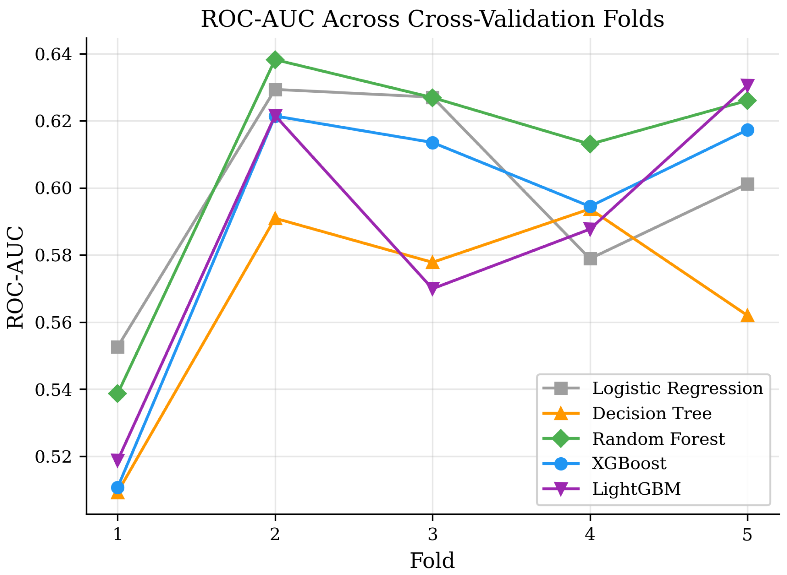
To assess the stability of these predictions over time,

Table 4. ROC-AUC by cross-validation fold for all five models.

Fold	LR	DT	RF	XGBoost	LightGBM
1	0.5526	0.5093	0.5387	0.5107	0.5187
2	0.6294	0.5910	0.6383	0.6215	0.6216
3	0.6271	0.5778	0.6269	0.6136	0.5700
4	0.5789	0.5938	0.6130	0.5945	0.5877
5	0.6012	0.5620	0.6261	0.6173	0.6305

details the performance across each temporal fold. Fold 1, which trains on the smallest dataset, consistently produces the weakest discrimination across all models (ROC-AUC near 0.51–0.54). Performance improves with additional training data, with folds 2–5 generally achieving an ROC-AUC of 0.56–0.63. Random forest achieved the highest individual fold score (0.6383, fold 2). The fold-level variation ranges from approximately 0.04 (LightGBM) to 0.08 (Decision Tree).

Figure 2 presents the fold-level trajectories. All models cluster within a ROC-AUC band of 0.51–0.64, with the weakest discrimination in fold 1 (limited training data). Random forest and logistic regression alternate as top performers across folds. XGBoost and LightGBM track closely throughout.

4.3. Feature Importance

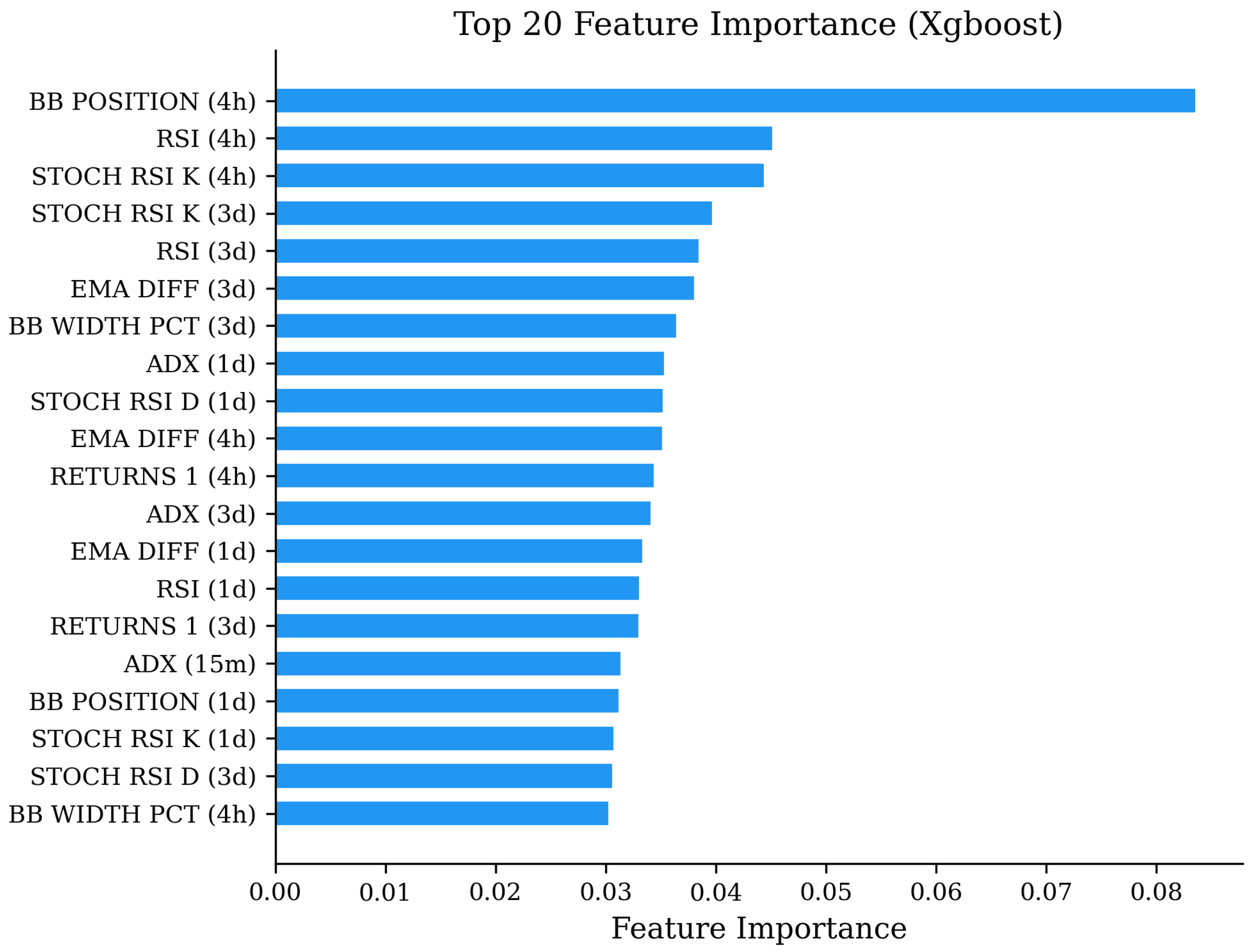
The feature importance is represented on

Table 5. Top 15 features by importance from XGBoost (best-performing tree-based model).

Rank	Feature	Timeframe	Importance	Share (%)
1	bb_position_4h	4 h	0.0837	8.3664
2	rsi_4h	4 h	0.0452	4.5220
3	stoch_rsi_k_4h	4 h	0.0445	4.4497
4	stoch_rsi_k_3d	3 d	0.0398	3.9754
5	rsi_3d	3 d	0.0385	3.8542
6	ema_diff_3d	3 d	0.0381	3.8124
7	bb_width_pct_3d	3 d	0.0365	3.6502
8	adx_1d	1 d	0.0354	3.5435
9	stoch_rsi_d_1d	1 d	0.0353	3.5281
10	ema_diff_4h	4 h	0.0353	3.5253
11	returns_1_4h	4 h	0.0345	3.4497
12	adx_3d	3 d	0.0342	3.4223
13	ema_diff_1d	1 d	0.0334	3.3437
14	rsi_1d	1 d	0.0332	3.3174
15	returns_1_3d	3 d	0.0331	3.3088

, which shows the 15 most important features of XGBoost. The 4-hour Bollinger Band position is the single strongest predictor (8.4% share), followed by the 4-hour RSI (4.5%) and the 4-hour Stochastic RSI K (4.5%). The 4-hour timeframe contributes three of the top five features, suggesting that the intermediate-timeframe regime context is the most discriminative signal.

Figure 3 displays the top 20 features in a bar chart. The 4-hour Bollinger Band position is the dominant feature, and the remaining features are distributed more evenly across timeframes. The dominance of the 4-hour Bollinger Band position (8.37%) and RSI suggests that intermediate-term volatility and momentum regimes are the most discriminative signals. This corroborates findings that volatility and momentum are amongst the most reliable predictive signals in financial machine learning. To provide a broader perspective, Table 5 aggregates these scores by timeframe.

4.4. Confusion Matrix

Table 6. Confusion matrix for Random forest (fold 5, n = 1158).

Actual \\ Predicted	Negative	Positive
Negative (0)	355	181
Positive (1)	284	338

shows the confusion matrix for the best-performing model on the final (largest) test fold.

4.5. Timeframe Contribution Analysis

Table 7. Timeframe ablation analysis: aggregate XGBoost feature importance by timeframe, computed as the sum of individual feature gain scores. The 4 h resolution contributes 32.84% of total importance, confirming its dominant role relative to finer (15-min) and coarser (daily, 3-day) temporal scales.

Timeframe	Features	Total Importance	Share (%)
4 h	9	0.33	32.84
3 d	9	0.28	27.78
1 d	9	0.26	25.95
15 m	10	0.13	13.43

aggregates XGBoost feature importance by timeframe. Importance is distributed more evenly across timeframes than might be expected, with the 4 h timeframe contributing the largest aggregate share due to the dominance of bb_position_4h. The 3-day and 1-day timeframes provide complementary context, while the 15 min timeframe—despite contributing 10 of 37 features—accounts for a smaller aggregate share, consistent with the interpretation that broader market regime features are more discriminative than short-term oscillator readings.

This timeframe-level aggregation constitutes an ablation-style analysis of each temporal resolution’s contribution to predictive performance. The 4 h scale provides approximately 2.5× the discriminative signal of the 15 min scale, while all four timeframes contribute meaningfully, the multi-resolution design cannot be reduced to any single scale without measurable loss.

4.6. Simplified Out-of-Sample Backtest

A simplified backtest is conducted on the last temporal fold (fold 5), which serves as a strictly out-of-sample test set. Each model is trained on folds 1–4 and generates predicted probabilities for the test samples. A strategy is then simulated that enters a position only when the predicted probability exceeds a threshold $\tau$ and uses each signal’s realized outcome as the average per-trade P&L from the label generation.

Table 8. Simplified out-of-sample backtest (last fold, Feb–December 2024). Avg Trade shows the mean per-trade P&L. Max DD is computed from the multiplicative compounding of sequential trades without capital constraints.

Strategy	$\mathit{\tau }$	Trades	Hit Ratio (%)	Avg Trade (%)	Max DD (%)
Rule-Based (all signals)	–	1158	44.82	0.08	−90.96
Logistic Regression	0.5	459	54.47	0.15	−55.78
Logistic Regression	0.6	163	53.37	0.37	−37.62
Logistic Regression	0.7	17	88.24	1.88	−0.25
Decision Tree	0.5	729	47.74	0.09	−77.25
Decision Tree	0.6	539	48.61	0.08	−69.92
Decision Tree	0.7	539	48.61	0.08	−69.92
Random Forest	0.5	622	54.34	0.16	−62.42
Random Forest	0.6	295	60.00	0.44	−46.84
Random Forest	0.7	43	65.12	0.46	−14.53
XGBoost	0.5	687	51.82	0.18	−62.40
XGBoost	0.6	454	58.37	0.34	−56.23
XGBoost	0.7	329	60.49	0.42	−46.78
LightGBM	0.5	613	52.85	0.21	−59.01
LightGBM	0.6	458	56.55	0.28	−56.34
LightGBM	0.7	265	59.25	0.31	−36.57

Note: The simplified backtest compounds individual trade P&L values sequentially without modeling capital constraints, position overlap, or execution costs. The average per-trade return is the most directly interpretable metric.

presents the results of the backtest. The number of trades decreases as $\tau$ increases from 0.5 to 0.7, whereas the hit ratio generally increases. At $\tau =0.7$, logistic regression achieves the highest hit ratio (88.2%) but with very few trades (17), while XGBoost maintains a more practical balance of 60.5% hit ratio with 329 trades. The unfiltered rule-based baseline achieved 44.8% hit ratio across all 1158 signals. Most ML-filtered strategies reduce the maximum drawdown relative to the unfiltered baseline, although the improvement is modest given the models’ overall low discriminative power.

4.7. Out-of-Sample Evaluation (2025 Holdout)

Table 9. 2025 out-of-sample models trained on full 2020–2024 data (6951 samples) and tested on 1136 independently generated 2025 samples.

Model	ROC-AUC	Accuracy	Precision	Recall	F1
Logistic Regression	0.6087	0.5801	0.5744	0.5423	0.5579
Decision Tree	0.5400	0.5150	0.5026	0.6919	0.5823
Random Forest	0.5862	0.5431	0.5321	0.5369	0.5345
XGBoost	0.5805	0.5819	0.5621	0.6523	0.6038
LightGBM	0.5785	0.5555	0.5414	0.5892	0.5643

presents the 2025 out-of-sample classification metrics. To provide the most stringent test of generalization, all five models are trained on the complete 2020–2024 dataset (6951 samples) and evaluated on independently generated 2025 data (1136 samples). The 2025 labels were produced using the identical simulation engine and were not used during any stage of model development. Logistic regression achieved the highest ROC-AUC (0.6087), followed by random forest (0.5862) and XGBoost (0.5805). The model ranking partially shifts compared to cross-validation: Logistic Regression moves from second to first, suggesting that its simpler linear decision boundary is slightly better for a fully unseen period. All five models maintain ROC-AUC above 0.54, confirming that modest discriminative ability persists into 2025, although the signal is weak.

Table 10. 2025 out-of-sample simplified backtest. Models trained on full 2020–2024 data and evaluated on 1136 independently generated 2025 signals.

Strategy	$\mathit{\tau }$	Trades	Hit Ratio (%)	Avg Trade (%)	Max DD (%)
Rule-Based (all signals)	–	1136	48.8556	0.0276	−91.1157
Logistic Regression	0.5	524	57.4427	0.1626	−65.9024
Logistic Regression	0.6	227	59.0308	0.2187	−43.2604
Logistic Regression	0.7	26	76.9231	0.7412	−9.6174
Decision Tree	0.5	764	50.2618	0.0591	−79.6342
Decision Tree	0.6	571	50.4378	0.0367	−69.2298
Decision Tree	0.7	417	52.2782	0.1881	−58.1003
Random Forest	0.5	560	53.2143	0.0456	−76.7217
Random Forest	0.6	278	58.2734	0.1729	−47.6467
XGBoost	0.5	644	56.2112	0.1915	−72.2415
XGBoost	0.6	344	55.8140	0.1631	−47.5467
XGBoost	0.7	60	70.0000	0.6772	−27.0580
LightGBM	0.5	604	54.1391	0.1544	−76.6870
LightGBM	0.6	308	61.6883	0.3591	−40.7486
LightGBM	0.7	51	58.8235	0.7667	−18.7858

shows the results of the 2025 out-of-sample backtest. At $\tau =0.7$, logistic regression achieved the highest hit ratio (76.9%) with 26 trades, while XGBoost reached 70.0% with 60 trades. The rule-based baseline without ML filtering achieved 48.9% hit ratio across all 1136 signals. ML-filtered strategies improve hit ratios relative to the unfiltered baseline, particularly at higher thresholds, although the trade-off between selectivity and trade count is more pronounced in ML-filtered strategies than in cross-validation. The modest improvements confirm that the ML filter provides a real but limited edge on unseen data.

4.8. Event-Driven Backtest

A full event-driven simulation is conducted on the 2025 out-of-sample period to complement the simplified backtest above. Unlike the simplified backtest, which sequentially compounds individual trade P&L values, the event-driven backtest models realistic trading conditions: capital allocation (100% of equity per position for single-asset BTC trading), compound interest (position size scales with current equity), entry slippage (0.1% cost applied to entry price), intra-bar stop-loss/take-profit execution using high/low prices, and a maximum of one concurrent position.

The XGBoost model trained on the full 2020–2024 dataset is used for signal generation within a two-phase hybrid strategy. In the first phase, the same rule-based entry condition used for label generation must be satisfied (Stochastic RSI K < 20, ADX > 25, EMA alignment); only candles meeting this filter are passed to the model. In the second phase, the model produces a predicted probability for the filtered candle; if this exceeds the threshold $\tau$, a long position is entered. It is therefore important to note that the event-driven backtest evaluates a hybrid strategy—a rule-based pre-filter combined with an ML probability gate—rather than a pure ML signal. The ML component is effectively learning to discriminate profitable from unprofitable outputs of the base rule, not to generate entry signals independently. Positions are exited when the candle’s low reaches the stop-loss price or the candle’s high reaches the take-profit price, following the same conservative priority used in label generation (stop-loss checked first).

Table 11. Top 5 event-driven backtest configurations on 2025 out-of-sample data, ranked by total return. The Sharpe ratio is annualized ($\sqrt{252}$). Max DD is the maximum peak-to-trough drawdown. Initial capital: $10,000.

SL (%)	TP (%)	$\mathit{\tau }$	Return (%)	Sharpe	Max DD (%)	Trades	Win Rate (%)
1.0	2.0	0.70	+35.97	0.14	−17.56	185	39.5
1.5	2.0	0.70	+29.19	0.12	−18.39	137	48.9
1.5	3.0	0.70	+28.78	0.11	−16.70	97	40.2
1.0	3.0	0.70	+25.38	0.11	−19.12	121	30.6
1.5	5.0	0.70	+20.16	0.08	−21.48	69	27.5

presents the top configurations ranked by total return on the 2025 out-of-sample period across 270 parameter combinations (6 SL × 9 TP × 5 thresholds).

The best configuration (SL = 1%, TP = 2%, $\tau$ = 0.7) achieves a +35.97% return with 185 trades and a maximum drawdown of −17.56%. The consistent appearance of $\tau =0.7$ across all top configurations confirms that higher probability thresholds improve economic outcomes by filtering out lower-confidence signals. The asymmetric risk-reward ratio (SL = 1%, TP = 2%) captures small but frequent gains, with a win rate of 39.5% compensated by the 2:1 reward-to-risk ratio.

These figures represent a gross upper bound on achievable returns, obtained before any transaction costs. The Sharpe ratios remain low (0.08–0.14) and maximum drawdowns of 17–22% indicate substantial risk even in this optimistic scenario. Crucially, the backtest does not model exchange fees (typically 0.1% per trade), which would reduce net returns by approximately 37 percentage points across 185 trades at 0.2% round-trip cost—likely erasing the entirety of the observed profit. The central implication is that models with ROC-AUC ≈ 0.57 cannot be expected to generate economically significant returns once realistic costs are incorporated, and transaction-cost modeling is an indispensable step before any deployment decision.

Table 12. Transaction cost sensitivity analysis for the best event-driven backtest configuration (SL = 1%, TP = 2%, $\tau$ = 0.7, 185 round-trip trades). Net return $=+35.97\%-(\mathrm{fee}\mathrm{rate}\times 2\times 185)$.

Fee Rate (Round-Trip)	Net Return (%)	Break-Even Trades
0.0% (no fees)	+35.97	—
0.1% per side	+17.47	—
0.2% per side	−1.03	185
0.3% per side	−19.53	124

presents a cost sensitivity analysis for the best configuration (SL = 1%, TP = 2%, $\tau$ = 0.7, 185 trades), illustrating how net return degrades across representative fee regimes.

5. Discussion

5.1. Model Comparison

The systematic comparison of five algorithms reveals that all models achieve modest but consistent discriminative ability, with ROC-AUC values ranging from 0.57 to 0.61. Random Forest achieved the highest average ROC-AUC (0.6086), followed by Logistic Regression (0.5978) and XGBoost (0.5915). Decision Tree achieved the lowest ROC-AUC (0.5668).

Although existing studies report high directional accuracies (often in the 0.70–0.80 range, compatible with ROC-AUC values well above 0.6), to the best of our knowledge, few studies explicitly publish ROC-AUC metrics alongside rigorous multi-timeframe alignment. Rehman et al. [63] achieved better results; our results are arguably more realistic because of strict prevention of look-ahead bias in multi-timeframe data alignment.

The performance differences between the top models are small (0.6086 vs. 0.5978 vs. 0.5915). With only five cross-validation folds, these differences are unlikely to be statistically significant. Bootstrap 95% confidence intervals computed from 1000 resamples of the fold-level ROC-AUC scores confirm this: Random Forest [0.576, 0.641] overlaps substantially with Logistic Regression [0.561, 0.635] and XGBoost [0.555, 0.628], supporting the conclusion that no algorithm is meaningfully superior to the others. The practical implication is that model choice matters less than data quality: all five algorithms achieve similar discrimination when given properly aligned multi-timeframe features and rigorous temporal validation.

Random Forest achieves the best cross-validated performance, consistent with Breiman [47]’s theoretical framework. Its bagging mechanism averages over de-correlated trees, offering lower variance than individual models. However, Logistic Regression achieves the highest 2025 holdout ROC-AUC (0.6087), suggesting that its simpler linear boundary generalizes slightly better to unseen periods—a finding that is consistent with the regularization benefits of linear models under distribution shift.

XGBoost and LightGBM provide competitive discrimination with the additional advantage of native feature importance through gradient-based splits [50]. Their sequential error-correction mechanism and built-in regularization make them attractive for larger datasets where non-linear patterns may be more prominent.

Decision Trees serve as an informative lower bound: their performance (ROC-AUC 0.5668) shows that individual decision boundaries extract limited predictive signal and that variance reduction through ensembling or boosting provides meaningful improvement.

5.2. Multi-Timeframe Feature Contributions

Feature importance analysis reveals that intermediate-timeframe features provide the strongest discriminative signal. The 4 h Bollinger Band position is the single most important feature (8.4% share), followed by 4 h RSI (4.5%) and 4 h Stochastic RSI K (4.5%). The 4-h timeframe contributes three of the top five features, suggesting that intermediate regime context is more discriminative than either short-term oscillators or longer-term momentum.

The importance distribution across timeframes is more balanced than might be expected, with all four timeframes contributing meaningfully. This finding validates the multi-timeframe design: models trained on only 15 min features would miss the majority of the discriminative signal provided by higher-timeframe context.

The prominence of Bollinger Band position—which measures where price sits relative to its recent range—suggests that the model captures mean-reversion dynamics at the 4 h scale. Oversold entries (Stochastic RSI K < 20 on 15 m) are more likely to succeed when the 4-hour Bollinger Band position indicates room for upward movement. The 3-day and daily features provide complementary context about broader market momentum, consistent with established multi-timeframe trading practice [26].

The superiority of 4 h features over the 15-min timescale reflects a well-known phenomenon in quantitative finance: entry signals at sub-candle resolution are inherently noisy because individual 15 min bars capture transient order-flow imbalances that often reverse within the next few candles. In contrast, 4-h indicators capture mean-reversion cycles that persist over multiple 15 min periods, providing the regime context needed to assess whether a given entry timing is structurally favorable. The 15-min oscillators confirm the precise moment of the entry (i.e., oversold readings) but lack the capacity to determine whether the broader market structure supports a sustained price recovery. The ablation analysis in Table 7 confirms that removing the 4 h features would eliminate approximately one-third of the model’s total discriminative signal.

5.3. Price-Level-Agnostic Design

The normalization of all features to percentage or ratio form is a deliberate design choice with important practical implications. Bitcoin’s price varied from approximately $5000 (March 2020) to over $60,000 (2021) during our study period. A model using raw MACD values would implicitly learn that a given MACD level indicates a particular market state when, in reality, this represents very different conditions at different price levels.

By expressing MACD as a percentage of price, Bollinger Band width as a percentage, and using only bounded oscillators (0–100 scale), we ensure that the feature space remains stationary across price regimes. This is essential for temporal cross-validation to be meaningful: the model must learn patterns that persist across different market conditions, not artifacts of changing price scales.

We use the term “price-level-agnostic” rather than “asset-agnostic” to be precise about the scope of this contribution. The pipeline eliminates dependence on absolute price levels, which is a necessary—but not necessarily sufficient—condition for cross-asset generalization. Other asset-specific factors (e.g., market microstructure and liquidity profiles) may influence transferability to other cryptocurrencies or asset classes. Empirical validation on additional assets (e.g., ETH/USDT) using the identical feature pipeline is identified as future work.

5.4. Temporal Validation and Overfitting Prevention

The expanding-window validation strategy provides realistic estimates of generalization performance. Unlike standard k-fold cross-validation, which violates temporal dependence and can leak future information into training data [22,61], our approach guarantees that every test observation occurs strictly after all training observations.

The relatively consistent performance across folds (after fold 1) suggests that the learned patterns, while weak, are genuinely persistent rather than artifacts of specific time periods. However, the overall modest discrimination (ROC-AUC 0.57–0.61) indicates that entry prediction from technical features alone is a fundamentally difficult problem, consistent with weak-form market efficiency arguments [24].

The ROC-AUC values observed in our study are substantially lower than the values above 0.80 is sometimes reported in the cryptocurrency prediction literature. We attribute this gap primarily to our strict prevention of look-ahead bias in multi-timeframe data alignment (see Section 5.6). Studies that align higher-timeframe indicators using open timestamps—a subtle but common practice—inadvertently allow the model to see future information, inflating apparent performance.

The 2025 out-of-sample evaluation provides evidence that the modest discriminative ability persists on unseen data. When trained on the full 2020–2024 dataset and tested on independently generated 2025 data, all five models maintain ROC-AUC above 0.54, with Logistic Regression achieving 0.6087. The mean ROC-AUC change from cross-validation to the 2025 holdout is small (approximately 0.01 for most models), suggesting stable but limited generalization. The shift in model ranking—Logistic Regression leading out-of-sample versus Random Forest leading cross-validation—may indicate that simpler decision boundaries generalize slightly better when trained on the full five-year dataset.

5.5. Market Regime Dynamics

During the 2020–2024 sample, Bitcoin traversed several distinct market regimes: a sharp COVID-19 sell-off and subsequent recovery in 2020; a parabolic bull run culminating near 69,000 USD in November 2021; and a deep 2021–2022 bear market with peak-to-trough drawdowns exceeding 70%, followed by a gradual recovery in 2023–2024 [63,64,65,66]. These dynamics are consistent with empirical analyses that document pronounced bull and bear phases in Bitcoin markets [63,67]. The 2025 out-of-sample period further stresses the models, as Bitcoin trades in a post-halving environment shaped by reduced block rewards, evolving market microstructure, and renewed institutional participation [66,68]. Over this holdout year, the ML-filtered strategy achieves a +35.97% event-driven return before costs on 185 trades (SL = 1%, TP = 2%, threshold = 0.7), concentrating exposure on a subset of high-confidence entry signals rather than full market exposure. Although realistic transaction costs would substantially reduce this gross performance, the positive out-of-sample result under such volatile conditions suggests that even modest discriminative ability can be economically meaningful when combined with appropriate risk management [64,67].

5.6. Comparison to Literature

Our results provide a sobering complement to the existing cryptocurrency prediction literature, while many studies report ROC-AUC values above 0.80 [4,30], our results—obtained with strict look-ahead bias prevention—suggest that realistic discriminative ability from technical features alone is more modest (ROC-AUC 0.57–0.61). This gap highlights the critical importance of proper multi-timeframe data alignment, which is rarely discussed in existing studies.

Our study avoids common pitfalls identified by Bailey et al. [22] and Harvey et al. [69]: we use temporal validation (not random splits), report all five models tested (not just the best), provide fold-level results (not just averages), and explicitly address multi-timeframe look-ahead bias. This transparent reporting provides a more realistic—if less impressive—picture of expected performance.

5.7. Multi-Timeframe Look-Ahead Bias: A Methodological Contribution

During the development of this study, we identified and corrected a subtle form of look-ahead bias specific to multi-timeframe feature engineering that, to our knowledge, has not been explicitly discussed in the literature. The issue arises when higher-timeframe indicators are merged with lower-timeframe data using backward-looking as-of joins.

In most OHLCV datasets, the timestamp field represents the candle’s open time. A 4 h candle opening at 08:00 and closing at 12:00 carries the timestamp 08:00, but its close price, RSI, MACD, and all derived indicators reflect information available only at 12:00. When this candle is merged with 15-minute data using a backward as-of join on the timestamp column, all 15 min candles between 08:00 and 11:59 receive indicator values that would not, in reality, be known until 12:00. This effectively grants the model 1–4 h of future information for 4-h features, 1–24 h for daily features, and 1–72 h for 3-day features.

The magnitude of this bias is substantial. Before correction, our models achieved cross-validated ROC-AUC values of 0.73–0.81; after correction, the same models achieved 0.57–0.61. This is approximately 0.20-point inflation shows that even well-designed validation strategies (temporal cross-validation, expanding windows) cannot protect against bias introduced at the feature construction stage.

The correction is straightforward: before the as-of merge, shift the higher-timeframe timestamp forward by the candle duration (e.g., add 4 h for 4 h candles and 1 day for daily candles). This ensures that the merge only matches candles that have fully closed before the decision point. We recommend that all multi-timeframe studies explicitly verify this alignment, as the bias is difficult to detect from classification metrics alone.

5.8. Limitations

Several limitations should be acknowledged:

• Single asset: The study focuses exclusively on Bitcoin. While the price-agnostic feature design is intended to generalize, empirical validation on other cryptocurrencies or asset classes is needed. Future validation on ETH/USDT and BNB/USDT using the identical pipeline, without retraining, would constitute a direct test of the price-level-agnostic design claim and assess whether the learned entry-signal patterns transfer across assets with different liquidity profiles and volatility regimes.
• Dataset size: The 6951 labeled samples, while sufficient for the algorithms tested, limit the complexity of models that can be reliably trained. Larger datasets from higher-frequency data or multi-asset labeling could support more complex architectures.
• Label quality: Labels are derived from a rule-based simulation with fixed entry conditions (Stochastic RSI < 20, ADX > 25, EMA alignment). Different entry conditions would produce different labels and potentially different results. The majority-vote aggregation mitigates sensitivity to specific stop-loss/take-profit parameters but not to the entry rule itself.
• Trading simulation limitations: The event-driven backtest models capital allocation, compound interest, slippage, and intra-bar execution but does not include exchange fees (typically 0.1% per trade), market impact, or partial fills. These costs would reduce net returns by approximately 37 percentage points for the best configuration (185 trades × 0.2% round-trip cost), potentially erasing most of the observed profit.
• Stationarity assumption: The model assumes that patterns learned from 2020 to 2024 data will persist. Cryptocurrency markets are known for regime shifts and structural changes that may invalidate historical patterns.
• Hybrid strategy architecture: The event-driven backtest evaluates a two-phase hybrid strategy, not a pure ML approach. Candles must first satisfy the rule-based entry condition before the ML probability gate is applied. Consequently, the ML component learns to filter the outputs of a specific base rule, and its performance is conditional on that rule’s characteristics. Alternative entry conditions would produce different label distributions, different model behaviors, and potentially different economic outcomes.
• Classical machine learning scope: This study evaluates five classical and ensemble classifiers. Deep learning architectures—including LSTM, GRU, temporal convolutional networks, and Transformer-based models—were excluded on sample-efficiency and interpretability grounds. With 6951 training samples, these architectures face an unfavorable parameter-to-sample ratio that limits their generalization potential on this dataset. However, this design choice means that the reported results cannot be directly compared with deep learning benchmarks, and the relative performance of recurrent or attention-based architectures under the same strict temporal validation framework remains an open empirical question.

5.9. Implications for Forecasting Applications

The prediction pipeline developed in this study has practical relevance for several forecasting use cases. Probabilistic classifiers can rank candidate entry signals by predicted confidence, providing a calibrated filtering layer for downstream decision systems. The multi-timeframe feature pipeline can serve as one component of a broader forecasting engine, combining ML-derived signals with fundamental analysis and portfolio-level risk constraints.

From a model evaluation perspective, the temporal cross-validation framework provides a template for stress-testing forecasting models before deployment. Practitioners and researchers increasingly require that ML forecasting systems demonstrate robustness to regime changes and out-of-sample degradation [28,29]. The expanding-window validation used here, which exposes the model to progressively longer historical periods, including the 2022 bear market, addresses this concern directly.

However, translating classification performance into a deployed forecasting system involves additional methodological considerations. Model outputs must be calibrated to produce reliable probability estimates. The relationship between probabilistic forecasts and economic outcomes depends critically on transaction costs, position sizing, and market microstructure—factors that are outside the scope of this paper but represent important steps for any applied ML-driven forecasting system.

5.10. Future Work

Several directions for future research emerge from this study:

• Cross-asset validation: Applying the identical 37-feature pipeline to other liquid cryptocurrencies (ETH, BNB, and SOL) and examining whether the price-level-agnostic design transfers without retraining.
• Transaction cost modeling: Extending the event-driven backtest to incorporate exchange fees, market impact, and partial fills to determine whether the gross upper-bound return of +35.97% yields any positive net return under realistic trading costs.
• Alternative data integration: Incorporating order-flow data (order book imbalance and trade intensity), on-chain metrics (network activity and exchange flows), and sentiment indicators (social media and news) to complement the technical feature set.
• Adaptive retraining: Investigating online learning or periodic retraining schedules that allow the model to adapt to regime changes without catastrophic forgetting of previously learned patterns.
• Ensemble stacking: Combining the five models evaluated here through stacking or blending to potentially achieve superior discrimination by exploiting the complementary strengths of different algorithm families.
• Deep learning benchmarking: Future work should evaluate LSTM, GRU, temporal convolutional networks, and Transformer-based architectures under the identical temporal validation framework used here—applying the same timestamp-shift alignment, expanding-window cross-validation, and 2025 out-of-sample holdout. This would establish whether deep learning models provide meaningful discriminative gains over gradient-boosted ensembles when look-ahead bias is rigorously controlled and would address the open question of whether the reported ROC-AUC ceiling of 0.61 is a property of the feature set or of the model family.

6. Conclusions

In this study, we evaluate five machine learning algorithms for Bitcoin market entry prediction using a 37-feature hierarchical multi-timeframe pipeline. The main conclusions are as follows:

• All models achieved modest but consistent discriminative ability (ROC-AUC 0.57–0.61), with Random Forest leading in cross-validation and Logistic Regression on the 2025 holdout. The narrow performance band suggests that model choice matters less than feature quality and temporal data alignment.
• Intermediate-timeframe (4-h) features dominate predictive signal, contributing 32.84% of total importance, with all four timeframes adding meaningful discriminative value. This validates the multi-timeframe design: a single-resolution model would sacrifice the majority of available signal.
• Multi-timeframe look-ahead bias is a critical and underappreciated source of performance inflation. We identified and corrected a specific bias in higher-timeframe data alignment that inflated ROC-AUC by approximately 0.20 points (from 0.60 to 0.80). Price-agnostic normalization of all features to percentages or bounded oscillators is equally essential to ensure temporal generalization across Bitcoin’s wide price range.
• The 2025 holdout confirms generalization, but economic significance requires transaction cost modeling. All five models maintain ROC-AUC above 0.54 out of 1136 independently generated 2025 samples. The event-driven backtest yields a gross return of +35.97%; after realistic round-trip fees (0.2% per trade), net returns turn negative, illustrating that ROC-AUC ≈ 0.60 is insufficient for economically significant returns without further refinement.
• The label generation approach based on majority-vote aggregation across 54 SL/TP combinations produces robust, cost-diverse training targets that align the classifier objective with practical trading viability rather than a single risk-reward scenario.

These results show that rigorous temporal validation and proper multi-timeframe data alignment are at least as important as algorithm selection or feature engineering for producing honest performance estimates. The substantial gap between the corrected results and values commonly reported in the literature suggests that look-ahead bias may be a pervasive issue in multi-timeframe prediction studies. Future work should extend this framework to multiple assets, incorporate transaction cost modeling to determine net profitability, and investigate alternative data sources (order flow and sentiment) to improve discriminative ability.

References

1. Nakamoto, S. Bitcoin: A Peer-to-Peer Electronic Cash System. Bitcoin.org. 2008. Available online: https://bitcoin.org/bitcoin.pdf (accessed on 7 January 2026).
2. Gandal, N.; Hamrick, J.; Moore, T.; Oberman, T. Price manipulation in the Bitcoin ecosystem. J. Monet. Econ. 2018, 95, 86–96. [Google Scholar] [CrossRef]
3. Makarov, I.; Schoar, A. Trading and arbitrage in cryptocurrency markets. J. Financ. Econ. 2020, 135, 293–319. [Google Scholar] [CrossRef]
4. Chen, J. Analysis of Bitcoin price prediction using machine learning. J. Risk Financ. Manag. 2023, 16, 51. [Google Scholar] [CrossRef]
5. Rathore, R.K.; Mishra, D.; Mehra, P.S.; Pal, O.; Hashim, A.S.; Uddin, M.; Algarni, A.D.; Krah, D. Real-world model for bitcoin price prediction. Inf. Process. Manag. 2022, 59, 102968. [Google Scholar] [CrossRef]
6. Giudici, P.; Abu-Hashish, I. What determines bitcoin exchange prices? A network VAR approach. Financ. Res. Lett. 2020, 28, 309–318. [Google Scholar] [CrossRef]
7. Arias-Oliva, M.; Pelegrín-Borondo, J.; Matías-Clavero, G. Variables influencing cryptocurrency use: A technology acceptance model in Spain. Front. Psychol. 2019, 10, 475. [Google Scholar] [CrossRef]
8. Chen, Z.; Li, C.; Sun, W. Bitcoin price prediction using machine learning: An approach to sample dimension engineering. J. Comput. Appl. Math. 2020, 365, 112395. [Google Scholar] [CrossRef]
9. McNally, S.; Roche, J.; Caton, S. Predicting the price of Bitcoin using machine learning. In Proceedings of the 26th Euromicro International Conference on Parallel, Distributed and Network-Based Processing (PDP); IEEE: New York, NY, USA, 2018; pp. 339–343. [Google Scholar] [CrossRef]
10. Kumbure, M.M.; Lohrmann, C.; Luukka, P.; Porras, J. Machine learning techniques and data for stock market forecasting: A literature review. Expert Syst. Appl. 2022, 197, 116659. [Google Scholar] [CrossRef]
11. Hutchinson, J.M.; Lo, A.W.; Poggio, T. A Nonparametric Approach to Pricing and Hedging Derivative Securities via Learning Networks. J. Financ. 1994, 49, 851–889. [Google Scholar] [CrossRef]
12. Liu, S.; Oosterlee, C.W.; Bohte, S.M. Pricing Options and Computing Implied Volatilities Using Neural Networks. Risks 2019, 7. [Google Scholar] [CrossRef]
13. Ruf, J.; Wang, W. Neural Networks for Option Pricing and Hedging: A Literature Review. J. Comput. Financ. 2020, 24, 1–46. [Google Scholar] [CrossRef]
14. Jaquart, P.; Dann, D.; Weinhardt, C. Short-term bitcoin market prediction via machine learning. J. Financ. Data Sci. 2021, 7, 45–66. [Google Scholar] [CrossRef]
15. Sebastião, H.; Godinho, P. Forecasting and trading cryptocurrencies with machine learning under changing market conditions. Financ. Innov. 2021, 7, 3. [Google Scholar] [CrossRef]
16. Kimoto, T.; Asakawa, K.; Yoda, M.; Takeoka, M. Stock market prediction system with modular neural networks. In Proceedings of the 1990 IJCNN International Joint Conference on Neural Networks; IEEE: New York, NY, USA, 1990; Volume 1, pp. 1–6. [Google Scholar] [CrossRef]
17. Krauss, C.; Do, X.A.; Huck, N. Deep neural networks, gradient-boosted trees, random forests: Statistical arbitrage on the S&P 500. Eur. J. Oper. Res. 2017, 259, 689–702. [Google Scholar] [CrossRef]
18. Gu, S.; Kelly, B.; Xiu, D. Empirical asset pricing via machine learning. Rev. Financ. Stud. 2020, 33, 2223–2273. [Google Scholar] [CrossRef]
19. Fischer, T.; Krauss, C. Deep learning with long short-term memory networks for financial market predictions. Eur. J. Oper. Res. 2018, 270, 654–669. [Google Scholar] [CrossRef]
20. Zhou, H.; Zhang, S.; Peng, J.; Zhang, S.; Li, J.; Xiong, H.; Zhang, W. Informer: Beyond efficient transformer for long sequence time-series forecasting. Proc. AAAI Conf. Artif. Intell. 2021, 35, 11106–11115. [Google Scholar] [CrossRef]
21. Dixon, M.F.; Klabjan, D.; Bang, J.H. Classification-based financial markets prediction using deep neural networks. Algorithmic Financ. 2017, 6, 67–77. [Google Scholar] [CrossRef]
22. Bailey, D.H.; Borwein, J.M.; López de Prado, M.; Zhu, Q.J. The Probability of Backtest Overfitting. J. Comput. Financ. 2017, 20, 39–69. [Google Scholar] [CrossRef]
23. López de Prado, M. Advances in Financial Machine Learning; John Wiley & Sons: Hoboken, NJ, USA, 2018. [Google Scholar]
24. Malkiel, B.G. The efficient market hypothesis and its critics. J. Econ. Perspect. 2003, 17, 59–82. [Google Scholar] [CrossRef]
25. Park, C.H.; Irwin, S.H. What do we know about the profitability of technical analysis? J. Econ. Surv. 2007, 21, 786–826. [Google Scholar] [CrossRef]
26. Hurst, J. The Profit Magic of Stock Transaction Timing; Prentice-Hall: Englewood Cliffs, NJ, USA, 1970. [Google Scholar]
27. Aronson, D.R. Evidence-Based Technical Analysis: Applying the Scientific Method and Statistical Inference to Trading Signals; John Wiley & Sons: Hoboken, NJ, USA, 2006. [Google Scholar]
28. Edwards, D. Risk Management in Trading: Techniques to Drive Profitability of Hedge Funds and Trading Desks, 1st ed.; John Wiley & Sons: Hoboken, NJ, USA, 2014. [Google Scholar]
29. Platanakis, E.; Urquhart, A. Portfolio management with cryptocurrencies: The role of estimation risk. Econ. Lett. 2019, 177, 76–80. [Google Scholar] [CrossRef]
30. Nakano, M.; Takahashi, A.; Takahashi, S. Bitcoin technical trading with artificial neural network. Phys. A Stat. Mech. Its Appl. 2018, 510, 587–609. [Google Scholar] [CrossRef]
31. Derbentsev, V.; Datsenko, N.; Stepanenko, O.; Bezkorovainyi, V. Forecasting cryptocurrency prices time series using machine learning approach. SHS Web Conf. 2019, 65, 02001. [Google Scholar] [CrossRef]
32. Jay, P.; Kalariya, V.; Parmar, P.; Tanwar, S.; Kumar, N.; Alazab, M. Stochastic Neural Networks for Cryptocurrency Price Prediction. IEEE Access 2020, 8, 82804–82818. [Google Scholar] [CrossRef]
33. Huang, J.Z.; Huang, W.; Ni, J. Predicting bitcoin returns using high-dimensional technical indicators. J. Financ. Data Sci. 2019, 5, 140–155. [Google Scholar] [CrossRef]
34. Jiang, Z.; Liang, J. Cryptocurrency portfolio management with deep reinforcement learning. In Proceedings of the 2017 Intelligent Systems Conference (IntelliSys); IEEE: New York, NY, USA, 2017; pp. 905–913. [Google Scholar] [CrossRef]
35. Kyriazis, N.A. A survey on empirical findings about spillovers in cryptocurrency markets. J. Risk Financ. Manag. 2019, 12, 170. [Google Scholar] [CrossRef]
36. Rebane, J.; Karlsson, I.; Denic, S.; Papapetrou, P. Seq2Seq RNNs and ARIMA Models for Cryptocurrency Price Prediction. In Proceedings of the 3rd SIGKDD Workshop on Mining and Learning from Time Series (MiLeTS 2018), London, UK, 19–23 August 2018. Extended Abstract Retrieved from DiVA Portal, Record diva2:1258222. [Google Scholar]
37. Livieris, I.E.; Kiriakidou, N.; Stavroyiannis, S.; Pintelas, P. An Advanced CNN-LSTM Model for Cryptocurrency Forecasting. Electronics 2021, 10, 287. [Google Scholar] [CrossRef]
38. Seabe, P.L.; Moutsinga, C.R.B.; Pindza, E. Forecasting Cryptocurrency Prices Using LSTM, GRU, and Bi-Directional LSTM: A Deep Learning Approach. Fractal Fract. 2023, 7, 203. [Google Scholar] [CrossRef]
39. Lo, A.W. Adaptive Markets: Financial Evolution at the Speed of Thought; Princeton University Press: Princeton, NJ, USA, 2017. [Google Scholar] [CrossRef]
40. Machado, J.; Neves, R.; Horta, N. Developing Multi-Time Frame Trading Rules with a Trend Following Strategy, using GA. In Proceedings of the Companion Publication of the 2015 Annual Conference on Genetic and Evolutionary Computation, New York, NY, USA, 11–15 July 2015; GECCO Companion ’15. Volume 55, pp. 765–766. [Google Scholar] [CrossRef]
41. Percival, D.B.; Walden, A.T. Wavelet Methods for Time Series Analysis; Cambridge University Press: Cambridge, UK, 2000. [Google Scholar]
42. Huang, N.E.; Shen, Z.; Long, S.R.; Wu, M.C.; Shih, H.H.; Zheng, Q.; Yen, N.C.; Tung, C.C.; Liu, H.H. The Empirical Mode Decomposition and the Hilbert Spectrum for Nonlinear and Non-Stationary Time Series Analysis. Proc. R. Soc. Lond. Ser. A Math. Phys. Eng. Sci. 1998, 454, 903–995. [Google Scholar] [CrossRef]
43. Stoltzfus, J.C. Logistic regression: A brief primer. Acad. Emerg. Med. 2011, 18, 1099–1104. [Google Scholar] [CrossRef]
44. Hastie, T.; Tibshirani, R.; Friedman, J. The Elements of Statistical Learning: Data Mining, Inference, and Prediction, 2nd ed.; Springer: New York, NY, USA, 2009. [Google Scholar] [CrossRef]
45. Loh, W.Y. Classification and regression trees. In Wiley Interdisciplinary Reviews: Data Mining and Knowledge Discovery; CRC: Boca Raton, FL, USA, 2011; Volume 1, pp. 14–23. [Google Scholar] [CrossRef]
46. Berry, M.J.A.; Linoff, G.S. Data Mining Techniques: For Marketing, Sales, and Customer Relationship Management, 2nd ed.; John Wiley & Sons: Hoboken, NJ, USA, 2004. [Google Scholar]
47. Breiman, L. Random forests. Mach. Learn. 2001, 45, 5–32. [Google Scholar] [CrossRef]
48. Ho, T.K. Random decision forests. In Proceedings of the 3rd International Conference on Document Analysis and Recognition; IEEE: New York, NY, USA, 1995; Volume 1, pp. 278–282. [Google Scholar] [CrossRef]
49. Chen, T.; Guestrin, C. XGBoost: A scalable tree boosting system. In Proceedings of the 22nd ACM SIGKDD International Conference on Knowledge Discovery and Data Mining, San Francisco, CA, USA, 13–17 August 2016; pp. 785–794. [Google Scholar] [CrossRef]
50. Friedman, J.H. Greedy function approximation: A gradient boosting machine. Ann. Stat. 2001, 29, 1189–1232. [Google Scholar] [CrossRef]
51. Ke, G.; Meng, Q.; Finley, T.; Wang, T.; Chen, W.; Ma, W.; Ye, Q.; Liu, T.Y. LightGBM: A Highly Efficient Gradient Boosting Decision Tree. In Proceedings of the Advances in Neural Information Processing Systems; Guyon, I., Luxburg, U.V., Bengio, S., Wallach, H., Fergus, R., Vishwanathan, S., Garnett, R., Eds.; Curran Associates, Inc.: Red Hook, NY, USA, 2017; Volume 30. [Google Scholar]
52. McKinney, W. Data structures for statistical computing in python. In Proceedings of the 9th Python in Science Conference, Austin, TX, USA, 28 June–3 July 2010; Volume 445, pp. 51–56. [Google Scholar]
53. Harris, C.R.; Millman, K.J.; van der Walt, S.J.; Gommers, R.; Virtanen, P.; Cournapeau, D.; Wieser, E.; Taylor, J.; Berg, S.; Smith, N.J.; et al. Array programming with NumPy. Nature 2020, 585, 357–362. [Google Scholar] [CrossRef]
54. Pedregosa, F.; Varoquaux, G.; Gramfort, A.; Michel, V.; Thirion, B.; Grisel, O.; Blondel, M.; Prettenhofer, P.; Weiss, R.; Dubourg, V.; et al. Scikit-learn: Machine learning in Python. J. Mach. Learn. Res. 2011, 12, 2825–2830. [Google Scholar]
55. Lam, S.K.; Pitrou, A.; Seibert, S. Numba: A LLVM-based python JIT compiler. In Proceedings of the Second Workshop on the LLVM Compiler Infrastructure in HPC; ACM: New York, NY, USA, 2015; pp. 1–6. [Google Scholar] [CrossRef]
56. CCXT. CCXT: CryptoCurrency eXchange Trading Library. 2024. Available online: https://github.com/ccxt/ccxt (accessed on 5 January 2026).
57. ARK Invest. Bitcoin Cycles, Entering 2025. 2024. Available online: https://www.ark-invest.com/articles/analyst-research/bitcoin-cycles-entering-2025 (accessed on 16 February 2026).
58. TA-Lib. TA-Lib: Technical Analysis Library. 2023. Available online: https://ta-lib.org (accessed on 9 January 2026).
59. Grinsztajn, L.; Oyallon, E.; Varoquaux, G. Why do tree-based models still outperform deep learning on tabular data? Proc. Adv. Neural Inf. Process. Syst. 2022, 35, 507–520. [Google Scholar] [CrossRef]
60. Shwartz-Ziv, R.; Armon, A. Tabular Data: Deep Learning is Not All You Need. Inf. Fusion 2022, 81, 84–90. [Google Scholar] [CrossRef]
61. Bergmeir, C.; Benítez, J.M. On the Use of Cross-Validation for Time Series Predictor Evaluation. Inf. Sci. 2012, 191, 192–213. [Google Scholar] [CrossRef]
62. Powers, D.M.W. Evaluation: From precision, recall and F-measure to ROC, informedness, markedness and correlation. arXiv 2020, arXiv:2010.16061. Available online: https://arxiv.org/abs/2010.16061 (accessed on 1 May 2026).
63. Rehman, M.U.; Ullah, S.; Shahzad, S.J.H. Bitcoin Volatility in Bull vs. Bear Markets: Insights from Analyzing On-Chain Metrics and Twitter Posts. PeerJ Comput. Sci. 2023, 9, e1750. [Google Scholar] [CrossRef]
64. Glassnode. A Bear of Historic Proportions. Glassnode Insights. 2022. Available online: https://insights.glassnode.com/2022-bear-of-historic-proportions/ (accessed on 5 February 2026).
65. Newhedge. Bitcoin Price Drawdown from ATH Chart. Newhedge Research. 2025. Available online: https://newhedge.io/bitcoin/price-drawdown (accessed on 7 February 2026).
66. NYDIG. Charting Drawdowns During Up Cycles. NYDIG Research Weekly. 2024. Available online: https://www.nydig.com/research/charting-drawdowns-during-up-cycles (accessed on 8 February 2026).
67. Bruzge, R.; Šapkauskienė, A. Asymmetries in Bitcoin Bull and Bear Market Phases. Financ. Res. Lett. 2024, 59, 104530. [Google Scholar]
68. Figment. Bitcoin in 2024 & Outlook 2025: Year in Review. Figment Research. 2025. Available online: https://www.figment.io/insights/bitcoin-in-2024-outlook-2025-year-in-review/ (accessed on 18 February 2026).
69. Harvey, C.R.; Liu, Y.; Zhu, H. … and the cross-section of expected returns. Rev. Financ. Stud. 2016, 29, 5–68. [Google Scholar] [CrossRef]
70. Fawcett, T. An introduction to ROC analysis. Pattern Recognit. Lett. 2006, 27, 861–874. [Google Scholar] [CrossRef]
Figure 1. Multi-timeframe feature engineering pipeline. Raw OHLCV series at four temporal resolutions are processed independently to compute technical indicators. A timestamp-shift procedure advances each higher-timeframe candle by one period before the as-of merge, ensuring only closed-candle values enter the feature vector and eliminating look-ahead bias. The resulting 37 features are all expressed as percentages, ratios, or bounded oscillators.
Forecasting 08 00040 g001
Figure 2. ROC-AUC across cross-validation folds for all five models. Later folds train on progressively larger datasets and test on more recent market periods.
Forecasting 08 00040 g002
Figure 3. Top 20 features by importance from XGBoost. Higher-timeframe momentum features (3-day and daily returns) dominate predictions, with 15 min features providing complementary entry-timing refinement.
Forecasting 08 00040 g003