Highlights
What are the main findings?
- The study introduces a novel Enhanced Peak (EP) loss function specifically designed to improve the prediction of peaks in time-series data. EP loss applies adaptive, asymmetric penalties for under- and over-estimations beyond a threshold, allowing the model to focus more effectively on extreme values.
- Through experiments on three diverse datasets, including NOx emissions (GRU model), streamflow (Transformer model), and gold prices (Transformer model), EPL consistently outperformed conventional loss functions (MSE, MAE, and Pinball loss) in overall accuracy and especially in capturing extremes or peaks.
What is the implication of the main finding?
- The EP loss function enhances model robustness and reliability for forecasting tasks involving highly variable or abrupt fluctuations, such as environmental emissions, hydrologic extremes, and financial market volatility.
- The superior performance of EP loss demonstrates its potential as a generalized framework for time-series modeling, enabling more accurate and peak-sensitive predictions across scientific, engineering, and economic applications.
Abstract
Time series models are considered among the most intricate models in machine learning. Due to sharp temporal variations, time series models normally fall short in predicting the peaks or local minima accurately. To overcome this challenge, we proposed a novel custom loss function, Enhanced Peak (EP) loss, specifically designed to pinpoint peaks and troughs in time series models, to address underestimations and overestimations in the forecasting process. EP loss applies an adaptive penalty when prediction errors exceed a specified threshold, encouraging the model to focus more effectively on these regions. To evaluate the effectiveness and versatility of EP loss, the loss function was tested on three highly variable datasets: NOx emissions, streamflow measurements, and gold price, implementing Gated Recurrent Unit and Transformer-based models. The results consistently demonstrated that EP loss significantly mitigates peak prediction errors compared to conventional loss functions, highlighting its potential for highly variable time series applications.
1. Introduction
Time series play a crucial role in capturing data variation over time, a feature that is especially important in industry and finance analyses [1]. The advent of artificial intelligence (AI) has transformed time series analysis and forecasting, enabling more accurate and efficient predictions across diverse domains [2]. By leveraging machine learning (ML) and deep learning (DL) techniques, AI can model complex temporal dependencies and patterns within data. These methods are widely applied in areas such as stock prices forecasting, engineering problem-solving, and industrial process optimization [3]. The capacity of AI to process large datasets and learn nonlinear relationships has made it a powerful and reliable tool for identifying trends and anomalies in time series data, ultimately supporting more robust decision-making and operational efficiency [4].
By nature, some time-series data exhibit high levels of fluctuation, making them difficult to analyze and model. Large variations and irregular patterns can introduce significant and unpredictable changes, complicating the modeling process [5]. Additionally, time-series data often contains outliers, abrupt shifts, or inconsistent patterns across observations. These irregularities can arise from various sources such as external shocks, measurement errors, or structural changes in the underlying system. Moreover, time-series data typically involves strong temporal dependencies, where current values are influenced by historical observations in complex ways. This temporal structure must be carefully captured to ensure accurate forecasting. Given these challenges, any model proposed for time-series prediction must be capable of identifying underlying patterns in the data while effectively handling noise, irregularities, and nonstationary behavior [6]. Traditional statistical models often fall short in addressing such complexity, highlighting the need for more flexible and adaptive approaches such as ML and DL, which can learn from data directly without relying on rigid assumptions [7].
Many approaches have been proposed for forecasting time series using ML and DL models, including Recurrent Neural Networks (RNNs), Long Short-term Memory (LSTM), Gated Recurrent Unit (GRU), and, more recently, Transformers. RNNs were a major research focus during the 1990s [3,8], developed specifically to process and analyze sequential data such as time series and language models. Unlike traditional feedforward neural networks, RNNs maintain a form of memory by passing information from one hidden state to the next, enabling the network to capture temporal dependencies across time steps. As a result, the output of an RNN is influenced not only by the current input but also by the sequence of prior inputs. This ability to model sequential relationships allows RNNs to capture long-term trends and complex patterns in time-series data, making them a powerful tool for forecasting tasks [3].
However, RNN models suffer from issues such as gradient explosion and vanishing gradient [9], which hinder their ability to learn long-term dependencies. To mitigate these problems, techniques like gradient clipping have been proposed [10]. A more robust solution emerged with LSTMs, which were specifically designed to address the limitations of standard RNNs [11]. In conventional RNNs, gradients can either become very small (vanish) or grow excessively large (explode) during backpropagation through time, making training unstable or ineffective. LSTMs introduced gating mechanisms—namely, the forget, input, and output gates—that control the flow of information through the network. These gates enable the model to retain or discard information selectively at each time step. In addition to the hidden state, LSTMs use a cell state, which acts as a memory buffer that helps preserve relevant historical information over long sequences. This architecture allows LSTMs to effectively capture long-term dependencies, making them more efficient and reliable for time-series forecasting compared to traditional RNNs [12].
Although LSTMs are effective at capturing long-term dependencies, their complex architecture, consisting of three gates (input, output, and forget) and a memory cell, makes them computationally expensive. To address this issue, Bengio et al. [13] introduced an RNN Encoder–Decoder architecture, which later evolved into the GRU. GRUs simplify the LSTM structure by using only two gates: the update gate, which determines how much information should be carried forward, and the reset gate, which controls how much past information should be forgotten. These two gates regulate the flow of information while maintaining a simpler structure, resulting in reduced computational cost compared to LSTMs [14]. Numerous studies comparing GRU and LSTM models have shown that GRUs often achieve similar or even superior performance to LSTMs [15,16], making them an efficient and competitive choice for sequence modeling tasks such as time-series forecasting [17].
RNNs, LSTMs, and GRUs process data sequentially, where each input is handled one time step at a time, with each step depending on the hidden state from the previous time step. This structure enables the models to effectively capture temporal dependencies within the data. However, the sequential nature of these models also limits their efficiency, as each computation must wait for the previous one to complete, leading to longer training times and limited parallelization. In contrast, Transformers represent a paradigm shift in sequence modeling. Introduced by Vaswani et al. [18], Transformers eliminate the need for sequential processing by leveraging a self-attention mechanism that captures dependencies between all elements in a sequence simultaneously. This architecture allows for efficient parallel computation and significantly improves the ability to model both short- and long-term dependencies. To compensate for the absence of recurrence, Transformers incorporate positional encoding, which provides information about the order of elements in the sequence.
The Transformer architecture was initially introduced for Natural Language Processing (NLP) tasks [19], but it has since demonstrated remarkable adaptability across a wide range of domains. In recent years, the potential of Transformers for time-series prediction has gained significant attention, largely due to their ability to effectively model long-range dependencies. Several studies have highlighted the superiority of Transformers in capturing complex temporal patterns. For example, Lim et al. [20] proposed a novel DL architecture called the Temporal Fusion Transformer (TFT), designed to improve both the accuracy and interpretability of multi-horizon time-series forecasting. A key innovation in TFT is the introduction of a Gated Residual Network (GRN), a flexible gating mechanism that allows the model to dynamically switch between linear and nonlinear processing pathways. To evaluate its performance, TFT was tested on multiple datasets, including traffic [21], electricity [22], retail, and financial volatility forecasting datasets, and consistently outperformed other benchmark models across all four domains.
In another study, Zhuo et al. [23] introduced a novel Transformer-based model called Informer, specifically designed for long-sequence time-series forecasting (LSTF). The model addresses several inefficiencies in traditional Transformer architectures, including scalability challenges, the complexity of the self-attention mechanism, high memory consumption, and limitations of the encoder–decoder structure. To overcome these issues, Informer introduces a ProbSparse self-attention mechanism, which selects only the most informative queries for attention computation, significantly reducing computational overhead. Additionally, Informer employs a Distilling Operation that compresses repetitive temporal patterns, allowing the model to focus more effectively on critical patterns during training. These innovations make Informer a highly efficient and scalable solution for LSTF tasks. The model’s superiority was demonstrated across various benchmark datasets, positioning Informer as a powerful tool for time-series prediction capable of capturing complex long-range temporal dependencies more effectively than traditional models.
LSTMs, GRUs, and Transformers have gained significant popularity for time-series prediction due to their ability to capture complex temporal dependencies and patterns. However, achieving optimal performance involves more than just the choice of model architecture. It also heavily relies on selecting an appropriate loss function. Loss functions play a crucial role in training by quantifying the discrepancy between predicted and actual values, guiding the model to minimize errors during backpropagation. While commonly used loss functions such as Mean Absolute Error (MAE) and Mean Squared Error (MSE) are effective in many situations, they may underperform in cases involving highly volatile data or abrupt changes over time. To better handle such challenges, researchers often design customized loss functions tailored to the specific complexities of their prediction tasks. These specialized functions can enhance model sensitivity to sudden variations and improve overall predictive accuracy in dynamic and irregular time-series environments.
One notable example of a customized loss function is the quantile regression loss function, also known as the pinball loss function, proposed by Koenker and Bassett [24]. This loss function asymmetrically penalizes underestimations or overestimations depending on the quantile of interest, enabling the model to focus on specific parts of the target distribution, such as the median, lower, or upper tails. Wang et al. [25] leveraged the pinball loss function in developing the Probabilistic Quantile Multiple Fourier Feature Network (QMFFNet), designed to forecast the temperature of Qinghai Lake. Given the inherent volatility of meteorological time series, conventional models often struggle to maintain accuracy. By incorporating the pinball loss, QMFFNet effectively captured the stochastic nature of the data. Experimental results demonstrated that QMFFNet outperformed baseline models, including MLP, LSTM, and GRU, highlighting the effectiveness of the pinball loss in managing complex, variable forecasting tasks. In a separate study, Kang et al. [26] applied the pinball loss function to the domain of electrical load forecasting. This work compared the performance of LSTM, RNN, and Gradient Boosting Regression Tree (GBRT) models. Among them, the LSTM model guided by the pinball loss achieved the highest predictive accuracy. Beyond improving forecast precision, this approach also enabled the generation of probabilistic forecasts, offering valuable insights into potential fluctuations in future electricity demand.
To further address the limitation of predicting peaks in high-variability time-series datasets through ML and DL with traditional loss functions such as MSE and MAE, this study introduces a novel loss function: the enhanced peak (EP) loss function. The EP loss function is specifically designed to reduce underestimation and overestimation errors at extreme values, thereby improving the accuracy of peak predictions. To assess the effectiveness of the EP loss function, a comprehensive experimental evaluation was conducted, benchmarking its performance against the pinball loss function and MSE, which serves as the baseline. Three complex and diverse time-series datasets were used in the evaluation: (i) a NOx emission dataset tracking nitrogen oxide (NOx = NO + NO2) emissions in a forested region of Iowa; (ii) a streamflow dataset comprising streamflow and precipitation measurements from the Iowa River Basin; and (iii) a financial dataset containing gold price data spanning from 1 January 2008 to 31 December 2023. Two ML models were employed: a GRU model for the NOx emissions dataset and a Transformer model for both the streamflow and gold price datasets. This multi-dataset, multi-model evaluation framework provides a robust assessment of EP’s generalizability and performance across varied time-series forecasting tasks.
The primary contribution of this study is the introduction of a novel loss function, specifically designed to enhance forecasting accuracy at peak values in high-variability time series datasets. Unlike the pinball loss function, which targets a specific quantile of the data distribution, the proposed EP loss function applies additional penalties to errors that exceed a defined threshold, thereby focusing more directly on peak prediction performance. Another distinguishing feature of the EP loss function is its separate treatment of underestimations and overestimations at peak values, regions where the largest discrepancies between predicted and actual values typically occur. By incorporating distinct penalty terms for over- and under-predictions, the EP loss function allows for asymmetrical error handling, offering more flexibility and precision than traditional symmetric loss functions. This threshold-based formulation enables the EP loss function to more effectively capture and penalize critical prediction errors, especially at extreme values. Empirical results from this study demonstrate that the EP loss function outperforms the pinball loss function in forecasting peaks. The efficacy of this new loss function is validated using real-world datasets, highlighting its potential as a robust tool for time series forecasting tasks involving abrupt changes and extreme values.
This paper is organized as follows. Section 2 introduces the GRU and Transformer models utilized in this study, along with a detailed description of the proposed EP loss function and the benchmark pinball loss function. Section 3 presents the datasets employed in this research, followed by model performance assessment. Finally, Section 4 concludes the paper and outlines directions for future work.
2. Methodology
This section outlines the methodology employed in this research. To address the limitations of RNNs in capturing long-term dependencies, this study utilizes GRU and Transformer models, two widely used approaches for time series analysis. The GRU model is applied to the NOx emission dataset, while the Transformer model is used for streamflow and financial datasets.
GRU models, which employ two gating mechanisms, can effectively capture both short- and long-term dependencies while being less computationally expensive than LSTMs. This efficiency makes GRUs particularly well-suited for time series prediction tasks, where computational resources and model simplicity are often key considerations. Transformers, on the other hand, represent a more recent innovation in time series analysis. Originally introduced for language modeling, Transformers differ from earlier models in their ability to process entire sequences simultaneously and prioritize inputs using an attention mechanism, without inherently considering sequential order. This characteristic gives Transformers a significant advantage over traditional models, particularly for tasks that require identifying complex dependencies. However, the sequential order of data is critical in time series analysis. To address this, positional encoding is incorporated into Transformer models, allowing them to preserve the sequential structure of the data while leveraging the benefit of self-attention.
To evaluate and compare the performance of the proposed loss function, EP, with the existing loss functions, such as pinball and Huber loss functions, conventional loss metrics such as MSE and MAE are used as baselines. Since only regression problems are considered in this study, the primary evaluation metrics are the coefficient of determination, denoted as the score, and the mean absolute percentage error (MAPE).
2.1. GRU
The GRU model was introduced by Bengio et al. [9]. Like the LSTM model, GRUs control the flow of information using gates; however, GRUs are simpler because they use one fewer gate than LSTMs, omitting the output gate. The two gates in a GRU are the reset gate and the update gate. With fewer gates, GRUs require fewer parameters, making them computationally more efficient and easier to train. The basic architecture of GRU cell is demonstrated in Figure 1. The typical mathematical formulation of a GRU is as follows:
where represents the update gate at time step t, is the reset gate vector, denotes the candidate activation vector, and is the final hidden state at the time step t. Furthermore, and represents sigmoid and hyperbolic tangent functions. W and R are weight matrices, and , , and are bias vectors. The inputs to the GRU cell in time step t is and while the output is that will be fed to the next cell as the input.
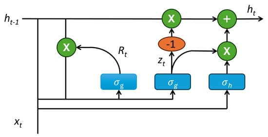
Figure 1.
Typical structure of a GRU cell.
GRUs, as RNN-based models, compute hidden states sequentially, with each state depending on the previous one, . This step-by-step processing enables GRUs to model temporal dependencies; however, it also limits their ability to capture very long-range relationships due to constrained memory capacity.
2.2. Transformers
To address the aforementioned challenges, Vawsani et al. proposed a novel model called the Transformer [18]. By eliminating recurrence and instead leveraging an attention mechanism, Transformers can capture global dependencies across input and output sequences while enabling parallel computation. The attention mechanism is the core component that allows the model to dynamically focus on different parts of the sequence. This design significantly improves efficiency and scalability, especially for long sequences. The Query, Key, and Value components are calculated by multiplying the input to , , and , respectively, where , , and are learned weight matrices. The attention mechanism determines the relevance between the queries and keys passed through the softmax function to produce probabilities. The output, which is the weighted sum of the values, is computed by a dot product in Equation (7). Figure 2 demonstrates the architecture of the transformer model.
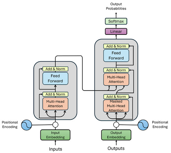
Figure 2.
Illustration of the Transformer architecture for time series forecasting. The left block represents the encoder with multi-head attention, feedforward layers, and residual connections, while the right block represents the decoder with masked multi-head attention and cross-attention layers. Positional encodings are added to input embeddings to capture temporal relationships.
Additionally, the transformer employs multi-head attention (Equation (8)), which improves the model’s ability to focus on different parts of the input sequence. Each head h is calculated using the attention equation, and then the outputs of all heads are concatenated by multi-head attention. Equation (9) defines the Feed-Forward Network, which is a crucial part of the encoder–decoder of transformers. It follows the multi-head attention and consists of two fully connected layers with a ReLU activation function between them. It is applied independently to each layer and helps capture non-linear relationships in the data. Equation (10) facilitates stable gradient flow during backpropagation and contributes to keeping the original input information.
Transformers process input tokens in parallel, which means that they do not prioritize order. This matter could become problematic in cases where the order is important, such as time series. Therefore, in addition to all the equations mentioned above, positional encoding is also used in the model. The positional encoding provides the model with the information, which enables the model to differentiate tokens based on their positions, ensuring that order-sensitive tasks, such as time series, are handled effectively. In the sinusoidal positional encoding, each position in the sequence is transformed into a vector using sine and cosine functions computed at multiple frequencies. This design enables the model to capture both absolute and relative positional information. The mathematical equation of positional encoding is provided in Equations (12) and (13), where denotes the position of the token in the sequence, i represents the index of the vector dimension, and indicates the dimensionality of the embedding.
2.3. Loss Functions
One of the key challenges in time series forecasting is making accurate predictions over data with high variability. Such data often exhibit sudden, large, and frequent changes over time, which complicates analysis and modeling. In these cases, adopting custom loss functions specifically designed to handle high-variability sequences can lead to significant improvements in performance. The pinball loss function [24] is one such approach, introduced to address this issue. By incorporating a quantile parameter, the pinball loss targets specific quantiles of the data distribution, making it especially useful for quantile regression. Equation (14) presents the mathematical formulation of the pinball loss function.
where y is the actual value, Y is the predicted value by the model, and q is the quantile variable that we give to the model as the input, and N is the number of samples.
The performance of the pinball loss function depends on the specified quantile. For instance, when , the loss behaves symmetrically and emphasizes minimizing the absolute error. However, if , the focus shifts toward penalizing underestimations more heavily while giving less attention to overestimations. In contrast, the proposed EP loss function addresses underestimations and overestimations separately, allowing the model to apply more targeted penalization, particularly around peak values.
In order to observe how well the EP loss function is performing on peak events, we also employed the Huber loss function [27] in our systematic comparison. The Huber loss function provides a balance between the sensitivity of the Mean Squared Error (MSE) to large errors and the robustness of the Mean Absolute Error (MAE) to outliers. It behaves quadratically for small residuals and linearly for large ones, controlled by a threshold parameter . This makes the Huber loss less sensitive to outliers than MSE while still maintaining smooth gradients, improving optimization stability. It is widely used in regression and time-series forecasting, where occasional extreme errors should not dominate the loss landscape. Equation (15) represents the Huber loss function.
Unlike the Huber loss, whose asymmetric behavior is determined solely by the magnitude of the residual, EP introduces a value-dependent asymmetry that becomes active specifically during peak regions of the target signal. This allows EP to apply proportional penalties for underestimation as the true value increases, ensuring that the model gives appropriate emphasis to high-intensity events that are often the most important in highly variable time series. Furthermore, EP includes a dedicated term for overestimation that enables controlled penalization of overestimation during peak events as well, providing flexible and balanced treatment of both types of errors in critical regions of the signal.
The EP loss incorporates three parameters: a threshold, which determines when penalization begins, and two penalization factors, which control the intensity of penalties for under- and overestimation. These two penalties, which we call the Underestimation factor and the overestimation factor, become activated when the model is faced with the corresponding scenario. To be more specific, the underestimation term triggers when the predicted value is lower than the actual value, and the overestimation term gets activated in the opposite condition. This conditional structure enables the loss function to adaptively penalize the error in a direction-aware manner. This structure encourages predictions to align more closely with actual values, thereby enhancing forecasting accuracy. The mathematical formulation of the EP loss function is presented below:
where is the underestimation factor, denotes the overestimation factor, T represents the threshold, and 1(.) is the indicator function (1 if the condition is true, 0 otherwise), used to activate penalty terms under specific conditions. The hyperparameters associated with the EP loss function were tuned using a grid search. This systematic exploration of the search space allowed us to identify the configuration that produced the best predictive performance while maintaining stability across multiple experiments.
To evaluate the effectiveness of the custom loss functions represented above, we employ MSE and MAE baselines. The model’s performance is compared using both these baseline loss functions and the custom loss functions. The mathematical formulations of MSE and MAE are given below:
2.4. Evaluation Metrics
To evaluate the performance of the model, the coefficient of determination ( score) was selected as the primary metric. In general, the score measures how well the model’s predictions capture the variance in the actual values. It typically ranges from 0 to 1, with higher values indicating better predictive performance. In addition to the score, the RMSE and Peak Recall [28] were also employed to assess the performance of the different loss functions. RMSE measures the average magnitude of the prediction error; it is sensitive to outliers and is therefore particularly useful when large deviations are undesirable. Smaller RMSE values indicate more accurate predictions. Peak Recall quantifies how effectively the model captures peak events above a specified threshold and measures the proportion of true peaks that the model successfully predicts. Moreover, the MAPE was employed to evaluate the model’s performance on the financial dataset. MAPE quantifies prediction accuracy as a percentage of the actual values, making it scale-independent and easily interpretable across different datasets. Recent studies have highlighted the importance of reporting uncertainty when evaluating machine learning models, as results from running the model for a single time may be sensitive to randomness in initialization, data shuffling, or training dynamics. Following the guidance of Rainio et al. [29], each experiment in this work was repeated 8–10 times with different random seeds, and we report the mean performance along with its standard deviation. This practice provides a more reliable representation of model stability and allows for statistically meaningful comparison across different loss functions. The mathematical formulations of the score and MAPE, RMSE, and Peak Recall are provided below:
Herein, τ denotes the threshold used for calculating Peak Recall. Because the objective of this study is to evaluate model accuracy specifically on peak events, we selected a consistent threshold of equal to 90 across all experiments. This allows us to focus on the highest 10% of the target distribution, which corresponds to the peak-value regime of greatest interest. Using a fixed and consistent ensures fair and comparable evaluation of peak-event performance among all models. In this study, model training and testing were carried out using Python 3.9.21 as the programming language. The experiments were conducted on a machine equipped with an Intel Core i7-6700HQ processor, an NVIDIA GeForce GTX 960M graphics card, and 16 GB RAM.
3. Result and Discussion
3.1. NOx Emission Prediction
Nitrogen oxides (NOx = NO + NO2) are reactive gases that play a pivotal role in atmospheric chemistry and environmental health. As an important form of nitrogen trace gas, NOx can be released from soils and may indirectly contribute to atmospheric warming. The dataset utilized in this study was collected in Iowa by the Environmental Protection Agency (EPA) [30]. The EPA operates approximately 360,000 sensors across the United States to monitor air quality, measuring criteria gases, particulates, meteorological parameters, toxins, ozone precursors, and lead. In Iowa, monitoring is conducted at three locations: the city of Des Moines, the city of Davenport, and a forest site located at 40°41′42.3″ N, 92°00′22.7″ W. For this study, we selected data from the forest site to minimize the influence of human activities and exclude the effects of fertilizers and irrigation.
Each data sample contains the following features: Latitude, Longitude, Date GMT, Time GMT, Sample Measurements, and Units of Measure. The measurements include air temperature (°F), relative humidity (%), and concentrations of NOx, CO, O3, and SO2 (parts per billion). Data have been recorded hourly since 1980. For this research, we analyzed records collected between January 2020 and September 2022, resulting in a total of 24,096 data points. To facilitate analysis, the dataset was divided into training, validation, and testing subsets: data from 2020 to 2021 were used for training; data from January to June 2022 for validation; and data from July to September 2022 was reserved for testing, as illustrated in Figure 3. It can be seen that there are NOx emission pulses that exhibit distinct temporal patterns, often associated with episodic environmental conditions. These variations highlight the importance of high-resolution temporal data in understanding the dynamics of trace gas emissions.
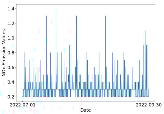
Figure 3.
Time series plot of NOx emission values in the test set, spanning from 1 July 2022, to 30 September 2022.
To predict future NOx emissions, we developed ML models using three key input features: historical and predicted air temperature, historical and predicted air moisture, and historical NOx emissions. A sliding window training framework was adopted, where data from a four-day period (96 hourly timesteps) was used to forecast NOx emissions over the subsequent six hours (6 hourly timesteps). Each timestep in the dataset represents one hour. In other words, the input features included 96 hourly values for past temperature, moisture, and NOx emissions, as well as 6 hourly forecasts for temperature and moisture. The model output consisted of predicted NOx emission values for the next 6 h.
A GRU-based model was implemented for the predication task. The architecture comprised three GRU layers with 64, 48, and 32 unies, respectively. Dropout regularization with a rate of 0.2 was applied after each GRU layer to reduce overfitting. Leaky ReLU was used as the activation function, and the output layer contained a single neuron to produce the NOx emission prediction. The model was trained using the Adam optimizer with a learning rate of 0.001 for over 50 epochs with a batch size of 96.
To establish a baseline, the model was trained using either MAE or MSE as the loss function. Although both loss functions yielded similar performance, the model trained with MAE was selected as the baseline due to its slightly better results on this dataset. Given the density of the data, only the final 15 days of predictions ar visualized for clarity, as shown in Figure 4a. The MAE-based model demonstrated reasonably accurate predictions across the lower and middle ranges of the data but struggled to align values at the peaks.
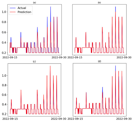
Figure 4.
Time series plot of NOx emission values comparison with predicted values implementing different loss functions: (a) MAE, (b) Pinball, (c) EP, and (d) Huber loss function.
Since most discrepancies between predicted and actual values occurred in the higher quantiles, we further evaluated the model using the pinball loss function with various quantile values. To obtain the optimum quantile value, a grid search with different values of quantile ranging from 0.6 to 0.9 was employed. Among these, a quantile of 0.7 produced better results, as shown in Figure 4b. Additionally, by investigating Figure 4a and identifying the point at which over- and under-estimations begin, we selected a threshold range from 0.3 to 0.6, ranging from 1 to 3, and from 1 to 3. Again, a grid search was used to find the best combination of hyperparameters. T = 0.4 along with the factors = 2.0 and = 1.5 provided the best performance and were therefore used to adjust the EP loss function. The results are displayed in Figure 4c. Similarly, a grid search was conducted to find the best δ for the Huber loss function. From values ranging from 0.1 to 1, δ = 0.3 yielded the best results and was therefore chosen for training the model.
Figure 4 illustrates that all three loss functions led to improved prediction accuracy compared to the baseline model trained with MAE. The Pinball loss helped the model better capture higher emission values that were underrepresented using MAE. Similarly, Huber loss function was able to capture most of the peak events but it was not as successful as pinball in that case. However, the most significant improvement was observed with the EP loss function, which not only reduced overall prediction error but also addressed the model’s tendency to underestimate peak NOx emissions. By explicitly penalizing over- and underestimation asymmetrically, the EP loss function enabled the model to produce more reliable forecasts during periods of elevated emissions. As shown in Figure 4c, this resulted in the best alignment between predicted and actual values, especially at critical peak regions, demonstrating the EP loss function’s effectiveness in enhancing model robustness and responsiveness to extreme values.
To further quantitatively evaluate model performance across different loss functions, scores, RMSE, and peak recall values for the entire test set and for a subset containing peak values greater than = 0.7 are compared in Table 1 and Table 2, respectively. Due to its inherent variability, the NOx emission dataset presents a more challenging forecasting task. Loss functions such as MAE and MSE, which treat all deviations equally, often fall short in capturing sudden variations in the trend. From the metric scores in Table 1, it is evident that ML models trained with the other custom loss functions outperform the baseline model trained with the MAE loss function. However, when it comes to predicting peak values, the model using the EP loss function shows superior performance. To be more specific, Table 2 demonstrates that although the overall metric scores for the models trained with Pinball, Huber, and EP loss functions are similar, the EP loss function shows a clear advantage in peak prediction tasks. By assigning distinct penalties to underestimation and overestimation, it effectively captures peak values.

Table 1.
Score, RMSE, and peak recall results for different loss functions on NOx emission dataset. Each model was run 8–10 times, and the table reports the mean value of each metric along with its corresponding standard deviation.
Table 2.
Score results for different loss functions on NOx emission dataset.
3.2. Streamflow Forecasting
The second dataset contains precipitation and streamflow data for the Iowa River Basin in Iowa. The streamflow data used in this study was simulated using the Hydrologic Modeling System (HEC-HMS) [31]. The primary input for HEC-HMS is rainfall events, which were generated using the Stochastic Storm Transposition (SST) framework [32], implemented via RainyDay, an open-source, Python-based software [33]. RainyDay utilized gridded Stage IV rainfall data (2002–2021) at a 4 km spatial and 1 h temporal resolution in 2021 to ensure accurate representation of complex rainfall patterns across the basin. A total of 200 synthetic rainfall events were derived from 72 h rainfall accumulations over the Iowa River Basin. These rainfall events served as input to the HEC-HMS semi-distributed hydrologic model, which simulated the corresponding streamflow at hourly intervals over a 20-day period for each event.
The above-mentioned process yielded labeled time series of rainfall and streamflow with a consistent temporal resolution of one hour for any location within the Iowa River Basin. However, for this specific study, the data was analyzed at the computational point in Iowa City. Each data sample comprises input sequences containing 60 h of historical rainfall and streamflow data, combined with 12 h future rainfall forecasts. The corresponding output sequences provide streamflow predictions extending up to 12 h ahead. The training dataset has 19,200 samples, with an additional 9600 samples reserved for the test set.
In our Transformer model, Time2Vec [34] was employed as the temporal encoding mechanism in place of traditional positional encoding. Time2Vec captures both linear and periodic patterns in the input sequence, enabling a more effective representation of the temporal dependencies. The temporal embeddings were concatenated with the original input features to form the input for the transformer layers. The architecture incorporated six attention blocks, each featuring a multi-head self-attention mechanism with eight heads and a head size of 128. These were followed by feed-forward dense layers. To mitigate overfitting, dropout with a rate of 0.2 and layer normalization were applied after each block. The model concluded with a dense output layer containing 12 neurons, corresponding to forecasts for the next 12 time steps.
For inference, the model generated outputs for all 12 future time steps simultaneously using a sequence-to-sequence approach, which enhances and reduces error accumulation over time. To further prevent overfitting, early stopping with a patience of 10 epochs was utilized. The model was optimized using the Adam optimizer with a learning rate of 0.0001. Prior to training, all input data were scaled to the [0, 1] range to ensure numerical stability and consistency.
To compare the performance of Transformer models across different loss functions in this study, we selected MSE as the baseline. Similar to other models, we utilized grid search when implementing loss functions to find the best set of hyperparameters. Therefore, a quantile of 0.8 was chosen for the pinball loss function. For the EP loss function, we set T = 0.8 with penalty factors of and assigned. Finally, for the Huber loss function δ = 0.4 was chosen. The parity plots of predicted vs. actual values for Transformer models using different loss functions are shown in Figure 5. The dashed lines represent perfect predictions in the figure. It can be seen that for the model using MSE as the loss function, the model failed to capture most of the peak values when the actual value rose to above 0.4, and overall, we are facing an underestimation situation. The parity plot Figure 5b shows that using the Pinball loss function, even though it can increase the underestimations, it still fails to fully capture the peak values, and a dispersed prediction for the values above 0.4 can be observed. Using Huber and EP loss functions, on the other hand, did the best performance in capturing underestimation and overestimation among all four of them. Although we can still see a small underestimation on the peak values, it greatly enhanced the model’s performance on peak prediction.
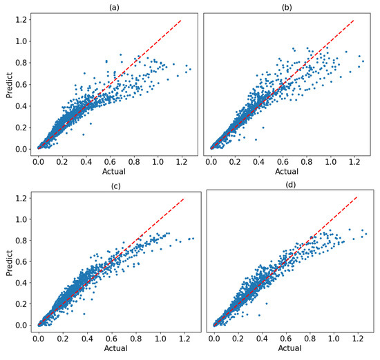
Figure 5.
The parity plots of predicted vs actual values for Transformer models using (a) MSE, (b) the Pinball loss function, (c) Huber, and (d) the EP loss function. Each blue dot represents a prediction–actual pair, and the red line denotes perfect agreement. Points lying below the line indicate underestimation, while points above the line indicate overestimation.
The resulting scores on the test set for each model, corresponding to the streamflow predictions at the 1 h lead time, and the 12 h lead time, and across the full 1–12 h lead time window, are presented in Table 3. The results show that the EP loss function yielded the best overall model performance compared to the other loss functions. Although all models performed similarly well at the 1 h lead time, the performance of the model using MSE dropped significantly at longer lead times compared to those using the other loss functions. Based on the results shown in Table 3, it can be observed that EP did a better job in forecasting the 1 h lead time, 12 h lead time, and also the full window. Both EP and Huber loss functions end up having close final results. However, EP performed slightly better than Huber loss function.
Table 3.
Performance metrics on the test set obtained from Transformer models trained with different loss functions. Each model was run 8 to 10 times, and the table reports the mean value of each metric together with its corresponding uncertainty standard deviation.
To further evaluate the loss functions and assess their ability to forecast peak values, Table 4 presents the scores calculated for actual values exceeding the threshold of 0.6, which is the same threshold used in the EP loss function. As shown, the model trained with the EP loss function outperforms those using the other loss functions. The drop of score shows that forecasting peak values is a particularly challenging task given the high variability in the data. While both the EP and Pinball loss functions yielded similar performance for the 1 h lead time prediction, the EP-based model maintained strong performance at the 12 h lead time. In contrast, the Pinball loss model exhibited a decline in performance due to error accumulation over longer lead times. Huber loss function, on the other hand, was able to capture peak event patterns similar to EP but similar to the previously mentioned results, EP performed slightly better. This matter shows that EP is capable of outperforming relevant loss functions that are specifically designed to treat underestimations. One of the key concepts that makes EP stand out in comparison to the other loss functions, such as pinball and Huber, is the advantage of treating underestimations and overestimations independently. This structure allows EP to penalize underestimation more heavily than overestimation or vice versa, depending on the application’s needs. In peak-sensitive time series problems, such asymmetric control is crucial because underestimating a peak often leads to much larger practical consequences than overestimating it. Unlike Huber, which applies the same symmetric penalty for positive and negative errors, and unlike Pinball loss, which applies a uniform asymmetry across the entire range of values, EP adjusts its penalty selectively and conditionally, activating stronger penalties only where the true signal enters a peak regime. This makes EPL particularly effective for data with high variability where the accurate reconstruction of extreme values is essential.
Table 4.
score calculated for the actual values above the threshold () for the streamflow dataset.
3.3. Gold Price Predictions
The third dataset used to evaluate the impact of loss functions on machine learning model performance is a financial dataset. Due to their high variability and unpredictability, financial datasets are well-suited as benchmarks in this study. We utilized historical gold price data sourced from the Yahoo Finance (yfinance) platform [35,36], covering the period from 1 January 2008, to 31 December 2023. This dataset includes daily adjusted close, close, open, high, and low prices, along with trading volume.
Given the relevance of price features, we selected the close price as both the input and target variable for prediction. Using only a single feature reduces model complexity and enhances interpretability, allowing for a clearer understanding of forecasting performance. The final dataset consisted of historical records collected at daily intervals, spanning 1 January 2008, to 31 December 2022, totaling 3774 data points. Among these, the first 2311 data points (1 January 2008 to 3 September 2017) were used for training, the next 500 data points (3 October 2017 to 3 July 2019) for validation, and the remaining 963 data points (from 3 August 2019 onward) for testing.
The data was preprocessed and normalized using the StandardScaler to improve the performance of the Transformer model. All the NaN (Not a Number) values were removed from the dataset set Historical data over a 90-day (three-month) window was used to predict the price for the next day, resulting in a total of 3679 data sequences, of which 963 belong to the test set. The same Transformer model architecture used for the streamflow prediction task was applied here, with the only modification being that the learning rate for the Adam optimizer was set to 0.001.
Herein, MSE was used as the baseline loss function. score along with MAPE, RMSE, and peak recall were employed as evaluation metrics to assess models’ performance. MAPE was selected alongside the other metrics to provide deeper insight into the model’s predictive accuracy on the financial dataset, as it expresses the average deviation between predicted and actual values in percentage terms. To find the best set of hyperparameters for EP, pinball, and Huber loss function, we conducted a grid search. For the EP loss function, the threshold was set to 2.0, with penalty factors and . For pinball loss function, a quantile of 0.7 was chosen, and finally, δ of 1.0 yielded the best result. Figure 6 and Figure 7 provide a detailed comparison of the test set predictions from Transformer models trained with different loss functions. Observations from these figures indicate that the MSE loss function struggles to capture important features of the data, particularly at peak values where it shows the largest deviations from the true values. This limitation stems from MSE treating all deviations equally, regardless of their magnitude or position in the data. In contrast, the Pinball loss function demonstrates improved performance compared to MSE but still struggles with peak predictions, especially in regions where the trend rises sharply. Huber loss function was able to capture most of the patterns in the time series both in the lower values, and in higher values, where the data is volatile. Our proposed loss function, however, exhibits strong potential in handling high-variability data. As shown in Figure 6d, the EP loss function more effectively aligns predictions with actual values at peaks, even in cases where the trend changes drastically. Table 5 represents the evaluation results for the four loss functions. Although Pinball loss function was able to improve the forecasting in compare with MSE as the loss function, but it could not outperform EP and Huber loss functions. As it is demonstrated, EP loss function was able to exhibit the best results in terms of both Score, RMSE, and MAPE. However, in terms of peak recall, Huber loss function yielded better results.
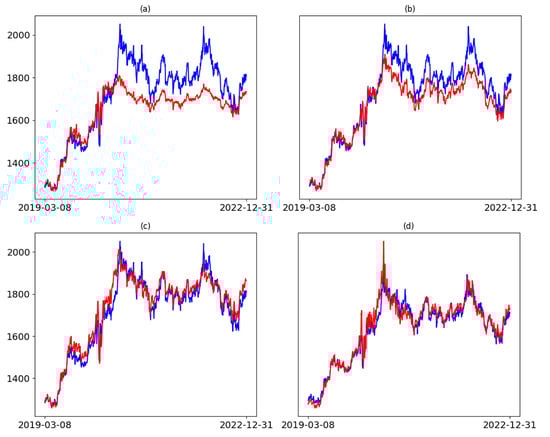
Figure 6.
The predicted gold price on the test set from Transformer models using (a) MSE; (b) the Pinball loss function; and (c) Huber loss function, and (d) EP loss function. In the plots, the blue lines demonstrate actual values, and the red lines represent the prediction.
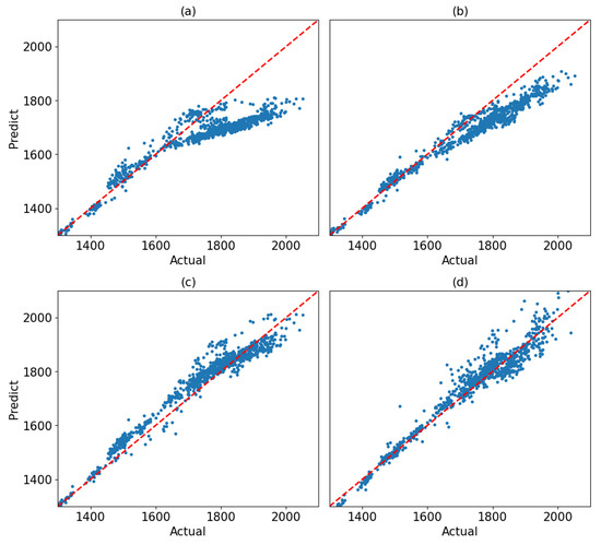
Figure 7.
The parity plots of predicted vs actual values for Transformer models on the financial dataset using (a) MSE, (b) the Pinball loss function, (c) Huber loss function, and (d) the EP loss function. Each blue dot represents a prediction–actual pair, and the red line denotes perfect agreement. Points lying below the line indicate underestimation, while points above the line indicate overestimation.
Table 5.
Performance metric values obtained from Transformer models trained with different loss functions on the financial dataset. Each model was run 8 to 10 times, and the table reports the mean value of each metric together with its corresponding standard deviation.
Table 6 contains the metric values using MSE, Pinball, EP, and Huber loss functions for the predictions above the threshold value. Basically, the threshold value determines where prediction and actual values start to go far off from each other. In this case, we chose 1800 as the threshold for this comparison, and it is the same value that was utilized for the threshold for the EP loss function. Based on the results, it can be observed that MSE, which is the baseline loss function, and Pinball did not perform a reasonable job for the values over the threshold. By establishing scores equal to −0.980 and 0.195, respectively, we can see how unpredictable they can perform in the peak values. EP and Huber loss functions, on the other hand, were able to display a significantly better performance by achieving scores 0.741 and 0.759, respectively. If we compare the results of these two loss functions, it can be seen that the difference between these two is negligible. Nevertheless, for Peak Recall, which specifically measures models’ performance over the peak events, EP was able to establish a slightly better performance.
Table 6.
scores, RMSE, Peak Recall, and MAPE values for the test samples higher than the threshold .
4. Conclusions and Outlooks
In this study, time series datasets with high variability were investigated. A new custom loss function named Enhanced Peak Loss function (EP) was proposed for improving prediction over peak forecasting. By acquiring two independent factors for underestimations and overestimations, EP can penalize inconsistencies with the actual values separately. To evaluate this loss function, the results from MSE and MAE were chosen as the baseline, and EPL’s performance was compared to the pinball loss function, which can improve underestimation or overestimation by adjusting its quantile value.
To demonstrate the advantage of the EP, their performance was measured over various datasets, including the NOx emission dataset, streamflow dataset, and Gold Price financial dataset. This collection of datasets was initially selected to span multiple application domains, such as environmental, hydrology, and finance to evaluate EP on diverse time series settings. The mentioned datasets are considered highly variable, meaning that the data is significantly volatile over time steps. This condition makes it demanding for models to capture temporal dependencies effectively. Our purpose was to introduce the EP loss function to overcome this issue. The EP loss function penalizes underestimation and overestimation after passing a specific threshold. This condition would promote the model’s ability to capture temporal dependencies over time steps, resulting in a more robust forecast.
EP was able to perform better than MSE, pinball, and Huber loss functions in all instances except one that Huber loss performed slightly better. Nevertheless, the difference was negligible. One reason for this is that pinball and Huber both have only one hyperparameter that limits their capability to treat underestimations and overestimations differently over peak values. EP, on the other hand, acquires a threshold and two terms for underestimation and overestimation, and can conform itself better in order to yield the best outcome. The prediction results prove the superiority of the EP over the other loss functions. The ability of EP to reduce error accumulation over time steps, while being tested on datasets from various domains, underscores its utility for real-world forecasting tasks, such as financial market predictions or energy demand modeling. This highlights its potential for broader adoption in domains requiring high temporal accuracy.
In spite of EP’s capability to conform itself dynamically to sharp peak variations, one of its limitations is the wide range of values that can be chosen for the hyperparameters. Since there is no range of values for the underestimation and overestimation factors, the model should be trained with various sets of hyperparameters in order to achieve the optimum results, which can be time-consuming in some cases.
Our future work involves validating the EP loss function’s applicability over more diverse datasets and enhancing its predictive ability not only on peak values but also across the entire dataset in order to reach ultimate forecasting performance.
Author Contributions
Conceptualization, S.T., M.H.S. and S.X.; methodology, S.T. and M.H.S.; software, M.H.S.; validation, M.H.S.; data curation, Z.W., S.T. and M.H.S.; writing—original draft preparation, Z.W., S.T. and M.H.S.; writing—review and editing, J.W. and S.X.; visualization, M.H.S.; supervision, J.W. and S.X.; project administration, J.W. and S.X.; funding acquisition, J.W. and S.X. All authors have read and agreed to the published version of the manuscript.
Funding
This material is based upon work supported by the National Science Foundation under Grant Numbers 2226936 and 2420405, as well as the U.S. Department of Education under Grant Number ED#P116S210005. Any opinions, findings, and conclusions or recommendations expressed in this material are those of the author(s) and do not necessarily reflect the views of the National Science Foundation and the U.S. Department of Education. Shaoping Xiao, Zhaoan Wang, and Jun Wang acknowledge the support from the University of Iowa OVPR Interdisciplinary Scholars Program for this study. Shaoping Xiao acknowledges the support from the University of Iowa OVPR professional development award. We also acknowledge the project support from the private-public-partnership (P3) program at the University of Iowa.
Data Availability Statement
The original NOx emission and gold price data presented in the study are openly available at https://github.com/MahanAbbassi/Nox-emission-and-gold-price-dataset (access on 1 December 2025). The Streamflow data is available for interested authors upon request from the corresponding author.
Conflicts of Interest
The authors declare no conflicts of interest.
Abbreviations
The following abbreviations are used in this manuscript:
| EP | Enhanced Peak Loss Function |
| MSE | Mean Squared Error |
| MAE | Mean Absolute Error |
| MAPE | Mean Absolute Percentage Error |
| RMSE | Root Mean Squared Error |
| GRU | Gated Recurrent Unit |
| LSTM | Long Short-Term Memory |
| HEC-HMS | Hydrologic Engineering Center–Hydrologic Modeling System |
References
- Zhang, G.P. A neural network ensemble method with jittered training data for time series forecasting. Inf. Sci. 2007, 177, 5329–5346. [Google Scholar] [CrossRef]
- Tealab, A. Time series forecasting using artificial neural networks methodologies: A systematic review. Future Comput. Inform. J. 2018, 3, 334–340. [Google Scholar] [CrossRef]
- Connor, J.T.; Martin, R.D.; Atlas, L.E. Recurrent neural networks and robust time series prediction. IEEE Trans. Neural Netw. 1994, 10, 240–254. [Google Scholar] [CrossRef]
- Yolcu, U.; Egrioglu, E.; Aladag, C.H. A new linear & nonlinear artificial neural network model for time series forecasting. Decis. Support Syst. 2013, 54, 1340–1347. [Google Scholar] [CrossRef]
- Jadon, S.; Milczek, J.K.; Patankar, A. Challenges and approaches to time-series forecasting in data center telemetry: A Survey. arXiv 2021, arXiv:2101.04224. [Google Scholar] [CrossRef]
- Dang, X.-H.; Shah, S.Y.; Zerfos, P. seq2graph: Discovering Dynamic Non-linear Dependencies from Multivariate Time Series. In Proceedings of the 2019 IEEE International Conference on Big Data (Big Data), Los Angeles, CA, USA, 9–12 December 2019; pp. 1774–1783. [Google Scholar] [CrossRef]
- Han, Z.; Zhao, J.; Leung, H.; Ma, K.F.; Wang, W. A Review of Deep Learning Models for Time Series Prediction. IEEE Sens. J. 2017, 21, 7833–7848. [Google Scholar] [CrossRef]
- Rumelhart, D.E.; Hinton, G.E.; Williams, R.J. Learning representations by back-propagating errors. Nature 1986, 10, 533–536. [Google Scholar] [CrossRef]
- Bengio, Y.; Simard, P.; Frasconi, P. Learning long-term dependencies with gradient descent is difficult. IEEE Trans. Neural Netw. 1994, 5, 157–166. [Google Scholar] [CrossRef]
- Pascanu, R.; Mikolov, T.; Bengio, Y. On the difficulty of training recurrent neural networks. PMLR 2013, 3, 1310–1318. [Google Scholar]
- Hochreiter, S.; Schmidhuber, J. Long Short-Term Memory. Neural Comput. 1997, 9, 1735–1780. [Google Scholar] [CrossRef] [PubMed]
- Astawa, N.G.A.; Pradnyana, P.B.A.; Suwintana, K. Comparison of rnn, lstm, and gru methods on forecasting website visitors. J. Hydrol. 2024, 628, 130504. [Google Scholar] [CrossRef]
- Cho, K.; van Merrienboer, B.; Gulcehre, C.; Bahdanau, D.; Bougares, F.; Schwenk, H.; Bengio, Y. Learning Phrase Representations using RNN Encoder–Decoder for Statistical Machine Translation. J. Abbr. 2008, 10, 142–149. [Google Scholar]
- Zarzycki, K.; Ławryńczuk, M. LSTM and GRU Neural Networks as Models of Dynamical Processes Used in Predictive Control: A Comparison of Models Developed for Two Chemical Reactors. Sensors 2021, 21, 5625. [Google Scholar] [CrossRef]
- Khandelwal, S.; Lecouteux, B.; Besacier, L. Comparing GRU and LSTM for Automatic Speech Recognition. LIG. 2016. Available online: https://hal.science/hal-01633254/document (accessed on 12 January 2025).
- Mateus, B.C.; Mendes, M.; Farinha, J.T.; Assis, R.; Cardoso, A.M. Comparing LSTM and GRU Models to Predict the Condition of a Pulp Paper Press. Energies 2021, 14, 6958. [Google Scholar] [CrossRef]
- Gurbuz, F.; Mudireddy, A.; Mantilla, R.; Xiao, S. Using a physics-based hydrological model and storm transposition to investigate machine-learning algorithms for streamflow prediction. J. Comput. Sci. Technol. Stud. 2022, 4, 11–18. [Google Scholar] [CrossRef]
- Vaswani, A.; Shazeer, N.; Parmar, N.; Uszkoreit, J.; Jones, L.; Gomez, A.N.; Kaiser, L.; Polosukhin, I. Attention is all you need. arXiv 2017, arXiv:1706.03762. [Google Scholar]
- Devlin, J.; Chang, M.; Lee, K.; Toutanova, K. BERT: Pre-training of Deep Bidirectional Transformers for Language Understanding. In Proceedings of the NAACL-HLT 2019, Minneapolis, MN, USA, 2–7 June 2019; pp. 4171–4186. [Google Scholar]
- Lim, B.; Arik, S.O.; Loeff, N.; Pfister, T. Temporal Fusion Transformers for interpretable multi-horizon time series forecasting. Int. J. Forecast. 2021, 37, 1748–1764. [Google Scholar] [CrossRef]
- Cai, L.; Janowicz, K.; Mai, G.; Yan, B.; Zhu, R. Traffic transformer: Capturing the continuity and periodicity of time series for traffic forecasting. Trans. GIS 2020, 24, 736–755. [Google Scholar] [CrossRef]
- Yu, H.; Rao, N.; Dhillon, I.S. Temporal regularized matrix factorization for high-dimensional time series prediction. Adv. Neural Inf. Process. Syst. 2016, 29, 847–855. [Google Scholar]
- Zhou, H.; Zhang, S.; Peng, J.; Zhang, S.; Li, J.; Xiong, H.; Zhang, W. Informer: Beyond efficient transformer for long sequence time-series forecasting. In Proceedings of the Thirty-Fifth AAAI Conference on Artificial Intelligence (AAAI-21), Virtually, 2–9 February 2021; Volume 35, pp. 11106–11115. [Google Scholar]
- Koenker, R.; Bassett, G. Regression Quantiles. Econometrica 1978, 46, 33–50. [Google Scholar] [CrossRef]
- Liu, S.; Deng, J.; Yuan, J.; Li, W.; Li, X.; Xu, J.; Zhang, S.; Wu, J.; Wang, Y. Probabilistic quantile multiple fourier feature network for lake temperature forecasting: Incorporating pinball loss for uncertainty estimation. Earth Sci. Inform. 2024, 17, 5135–5148. [Google Scholar] [CrossRef]
- Wang, Y.; Gan, D.; Sun, M.; Zhang, N.; Lu, Z.; Kang, C. Probabilistic individual load forecasting using pinball loss guided LSTM. Appl. Energy 2019, 235, 10–20. [Google Scholar] [CrossRef]
- Huber, P.J. Robust Estimation of a Location Parameter. Ann. Math. Stat. 1964, 35, 73–101. [Google Scholar] [CrossRef]
- Khoshvaght, A.; Farid, F.; Chen, Y.; Fenton, N.E. A Critical Review on Selecting Performance Evaluation Metrics for Supervised Machine Learning Models. Inf. Sci. 2025, 674, 119041. [Google Scholar]
- Rainio, K.; Beliaev, M.; Ilmonen, P. Evaluation Metrics and Statistical Tests for Machine Learning. Sci. Rep. 2024, 14, 6086. [Google Scholar] [CrossRef]
- Wang, Z.; Xiao, S.; Reuben, C.; Wang, Q.; Wang, J. Soil NOx Emission Prediction via Recurrent Neural Networks. Comput. Mater. Contin. 2023, 77, 285–297. [Google Scholar] [CrossRef]
- Tofighi, S.; Gurbuz, F.; Mantilla, R.; Xiao, S. Advancing Machine Learning-Based Streamflow Prediction Through Event Greedy Selection, Asymmetric Loss Function, and Rainfall Forecasting Uncertainty. Appl. Sci. 2025, 15, 11656. [Google Scholar] [CrossRef]
- Wright, D.B.; Smith, J.A.; Villarini, G.; Baeck, M.L. Estimating the frequency of extreme rainfall using weather radar and stochastic storm transposition. J. Hydrol. 2013, 488, 150–165. [Google Scholar] [CrossRef]
- Wright, D.B. RainyDay: Rainfall Hazard Analysis System. Github Repos. 2019. Available online: https://github.com/danielbwright/RainyDay (accessed on 12 January 2025).
- Kazemi, S.M.; Goel, R. Time2vec: Learning a vector representation of time. arXiv 2019, arXiv:1907.05321. [Google Scholar] [CrossRef]
- Yahoo Finance. Historical Gold Prices. Yahoo Finance. Available online: https://finance.yahoo.com (accessed on 12 January 2025).
- Aroussi, R. yfinance: Download Market Data from Yahoo! Finance’s API. Github Repos. 2019. Available online: https://github.com/ranaroussi/yfinance (accessed on 12 January 2025).


Disclaimer/Publisher’s Note: The statements, opinions and data contained in all publications are solely those of the individual author(s) and contributor(s) and not of MDPI and/or the editor(s). MDPI and/or the editor(s) disclaim responsibility for any injury to people or property resulting from any ideas, methods, instructions or products referred to in the content. |
© 2025 by the authors. Licensee MDPI, Basel, Switzerland. This article is an open access article distributed under the terms and conditions of the Creative Commons Attribution (CC BY) license (https://creativecommons.org/licenses/by/4.0/).