Forecasting the U.S. Renewable-Energy Mix with an ALR-BDARMA Compositional Time-Series Framework

Abstract

Accurate forecasts of the U.S. renewable energy consumption mix are essential for planning transmission upgrades, sizing storage, and setting balancing market rules. We introduce a Bayesian Dirichlet ARMA model (BDARMA) tailored to monthly shares of hydro, geothermal, solar, wind, wood, municipal waste, and biofuels from January 2010 through January 2025. The mean vector is modeled with a parsimonious VAR(2) in additive log ratio space, while the Dirichlet concentration parameter follows an intercept plus five Fourier harmonics, allowing for seasonal widening and narrowing of predictive dispersion. Forecast performance is assessed with a 61-split rolling origin experiment that issues twelve month density forecasts from January 2019 to January 2024. Compared with three alternatives (a Gaussian VAR(2) fitted in transform space, a seasonal naive approach that repeats last year’s proportions, and a drift-free ALR random walk), BDARMA lowers the mean continuous ranked probability score by 15 to 60 percent, achieves componentwise 90 percent interval coverage near nominal, and maintains point accuracy (Aitchison RMSE) on par with the Gaussian VAR through eight months and within 0.02 units afterward. These results highlight BDARMA’s ability to deliver sharp and well-calibrated probabilistic forecasts for multivariate renewable energy shares without sacrificing point precision.

1. Introduction

Electric-sector decarbonization hinges not only on expanding renewable output but also on anticipating how the mix of generation technologies will evolve. Hydropower, wind, solar, biomass, and geothermal differ sharply in marginal cost, intermittency, and siting constraints; therefore, reliable medium-term mix forecasts shape transmission expansion, storage sizing, and market design [1,2,3]. Renewables already supply about one-fifth of U.S. utility-scale electricity and their share is expected to double before 2050, making the coherence and accuracy of share forecasts more important than ever.

Shares are compositional: they are bounded between zero and one and must sum to unity. Forecasting each component in isolation, as is common with univariate ARIMA or machine learning regressions [4,5], yields incoherent predictions that may turn negative or exceed 100% [6]. Aitchison’s log-ratio geometry provides a principled fix [7]. Early multivariate illustrations such as the VAR for geological compositions in Billheimer et al. [8] and the state-space model of Snyder et al. [9] demonstrate that standard Gaussian machinery works once data are mapped to real space. Still, Gaussian log-ratio models often overstate predictive dispersion and ignore seasonally varying volatility.

Therefore, recent research models the composition itself. A Dirichlet ARMA process was proposed by Zheng et al. [10], a dynamic Dirichlet–multinomial filter by Koopman et al. [11], and a deep hierarchical Dirichlet forecaster by Das et al. [12]. In the cross-sectional domain, Morais et al. [13] showed that Dirichlet and compositional regression can outperform traditional attraction models when explaining brand market shares, underscoring the versatility of simplex-based methods. A direct antecedent to the present study is the Bayesian Dirichlet ARMA (BDARMA) framework from [14,15], subsequently explored with shrinkage priors for trading-sector shares by Katz et al. [16], which we adopt here as the data model for a new application to the U.S. renewable energy mix.

Applications to energy shares remain limited but growing. Compositional VAR and ARMA models as well as more recent regional optimization studies have been used to project national and subnational energy structures in China, the USA, and Canada [17,18,19,20]. Grey-system and hybrid approaches, such as adaptive discrete grey models and MGM–BPNN–ARIMA designs for broad-mix or bio-energy forecasting, further boost accuracy while respecting the simplex constraint [21,22,23]. Machine learning work, such as the LSTM study by Ma et al. [24] and logistic growth analysis of U.S. energy trajectories by Harris et al. [25], underline the need to tame nonlinearities; however, they still rely on ad hoc renormalization.

We apply the Bayesian Dirichlet ARMA framework to the seven-component U.S. renewable energy mix measured monthly from 2010 to 2024, a dataset with pronounced seasonality and secular trends hitherto unaddressed in the Dirichlet literature. Forecasting skill is benchmarked against three alternatives: a Gaussian VAR(2) in additive log-ratio space with identical Fourier dummies, a seasonal naïve approach that repeats the mix observed twelve months earlier, and a drift-free ALR random walk. A 61-split rolling protocol produces 732 out-of-sample density forecasts and shows that the Dirichlet model attains the strongest probabilistic performance while maintaining the VAR’s point accuracy. A full-sample forecast to early 2026 projects wind and solar surpassing one-third of renewable generation, providing a coherent picture for transmission and storage planning.

The remainder of the paper is organized as follows: Section 2 describes the EIA data and seasonal covariates; Section 3 presents the BDARMA and benchmark models; Section 4 details the rolling evaluation protocol and scoring rules; results are discussed in Section 5; and Section 6 concludes with policy implications and avenues for future research. A complementary robustness analysis aligned with the EIA STEO definitions is presented in the Supplementary Materials (Sections S1 and S2).

2. Data

The empirical analysis relies on the EIA monthly renewable energy consumption dataset. We retain $T=181$ consecutive months from January 2010 through January 2025. Each observation is a seven-part composition ${\mathbf{y}}_t={(y_{t,\mathrm{hyd}},y_{t,\mathrm{geo}},y_{t,\mathrm{sol}},y_{t,\mathrm{win}},y_{t,\mathrm{woo}},y_{t,\mathrm{was}},y_{t,\mathrm{bio}})}^{\top }\in {\mathcal{S}}_7,$ where shares are obtained by dividing each raw series by their monthly total.

Additive-log-ratio (ALR) coordinates. Throughout, we analyze the seven-part composition in additive-log-ratio form

$$\begin{array}{c}\hfill {\mathbf{e}}_t=alr\left({\mathbf{y}}_t\right)={\left(log\frac{y_{t,\mathrm{hyd}}}{y_{t,\mathrm{bio}}},log\frac{y_{t,\mathrm{geo}}}{y_{t,\mathrm{bio}}},log\frac{y_{t,\mathrm{sol}}}{y_{t,\mathrm{bio}}},log\frac{y_{t,\mathrm{win}}}{y_{t,\mathrm{bio}}},log\frac{y_{t,\mathrm{woo}}}{y_{t,\mathrm{bio}}},log\frac{y_{t,\mathrm{was}}}{y_{t,\mathrm{bio}}}\right)}^{\top }\in {\mathbb{R}}^6,\end{array}$$

(1)

where biofuels serve as the common denominator (reference part). The inverse map ${alr}^{-1}:{\mathbb{R}}^6\to {\mathcal{S}}_7$ restores a share vector via $y_{t,j}=exp\left(e_{t,j}\right){\left[1+{\sum }_{k=1}^{6}exp\left(e_{t,k}\right)\right]}^{-1}$ for $j\le 6$ and $y_{t,\mathrm{bio}}={\left[1+{\sum }_{k=1}^{6}exp\left(e_{t,k}\right)\right]}^{-1}$. We write $e_{t,j}$ for the j-th ALR coordinate and collect them as $e_1,\dots ,e_6$ when no time index is needed.

2.1. Electric-Power-Only Benchmarking

For comparisons to the EIA–STEO industry baseline, we also construct an electric-power-only view (hydro, geothermal, solar = utility-scale + small PV, wind, wood, waste) with monthly closure to the simplex. Implementation details and the strict vintaging rule are in the Supplementary Materials (Section S1).

2.2. Exploratory Data Analysis

Figure 1 highlights two macro-patterns in the sample: (i) pronounced asymmetric intra-annual seasonality, and (ii) a medium-run reallocation of market share from hydro to wind and solar.

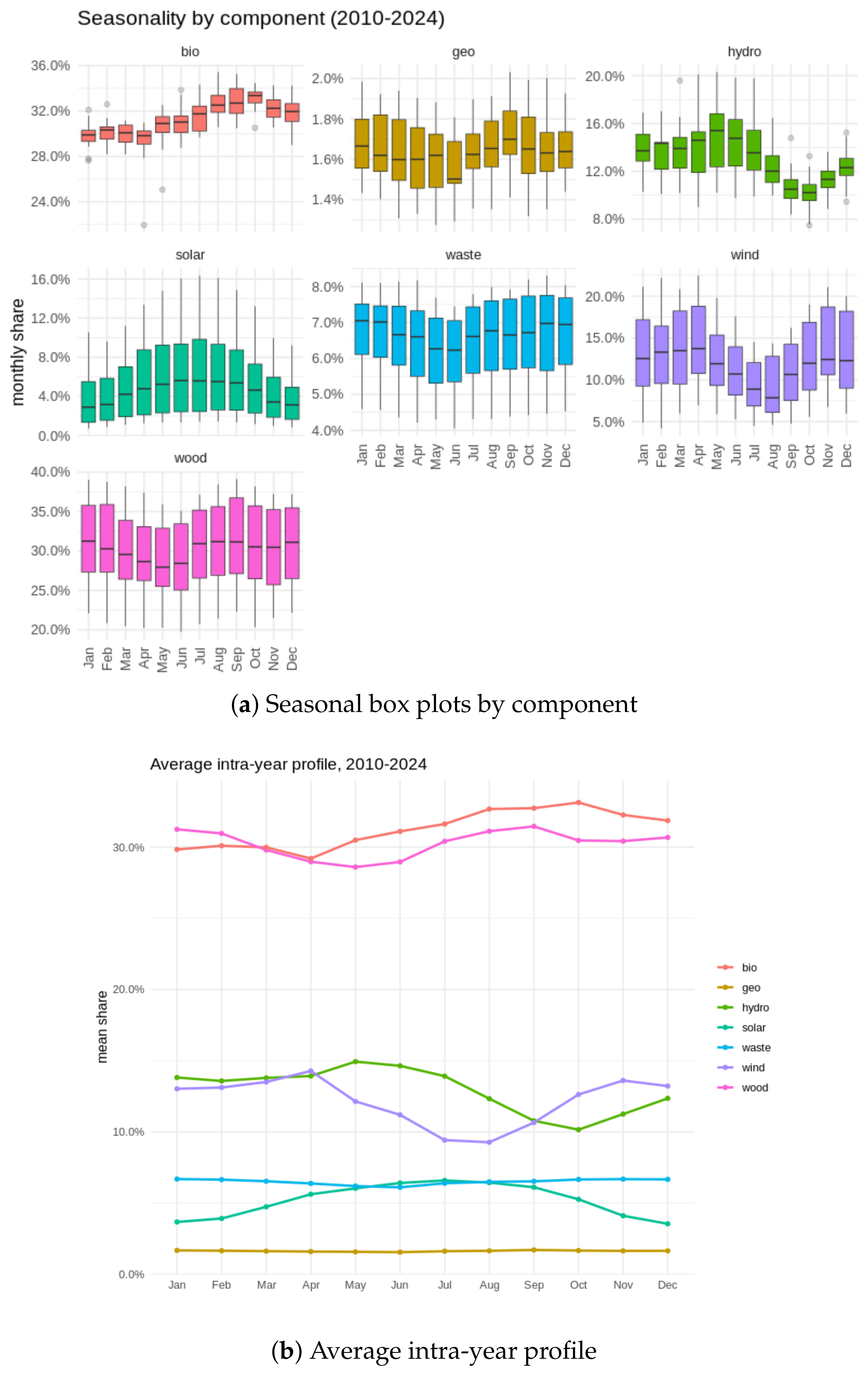
Panel (a) of Figure 2 shows componentwise box plots of monthly shares for 2010–2024; panel (b) traces the mean intra-year profile. Hydro exhibits the largest seasonal swing, peaking in April–May and troughed in late summer, while wind follows a bimodal winter/autumn pattern and solar the mirror image with a July plateau. Biomass, geothermal, and waste are comparatively flat, with median intra-year movements below 1 pp.

Figure 3a plots the correlation matrix of the six ALR coordinates $e_1,\dots ,e_6$ (biofuels as reference). Solar and wind move almost one-for-one relative to biofuels (${\rho }_{e_3,e_4}=0.97$), whereas hydro and wind are strongly anti-correlated (${\rho }_{e_1,e_4}\approx -0.86$). Panel (b) confirms that these pairwise relations are nonlinear, displaying the characteristic banana-shaped clouds induced by log-ratio geometry.

Table 1. Component means and dispersion, 2010–2024 (percent of total renewables).

	Hydro	Geo	Solar	Wind	Wood	Waste	Bio
Mean (%)	13.0	1.64	5.20	12.2	30.3	6.51	31.2
SD (%)	2.63	0.17	3.87	4.65	5.10	1.15	1.86
Q1 (%)	10.9	1.50	1.91	8.48	26.4	5.54	30.1
Q3 (%)	14.8	1.77	7.53	15.1	35.1	7.48	32.5
Min (%)	7.51	1.28	0.73	4.18	19.7	4.05	22.0
Max (%)	20.3	2.03	16.3	22.5	39.1	8.31	35.4

shows wide dispersion differences: hydro ranges from $7.5\%$ to $20.3\%$ (SD $=2.6$ pp), geothermal is quasi-deterministic (SD $=0.17$ pp), and wood the most volatile component (SD $=5.1$ pp).

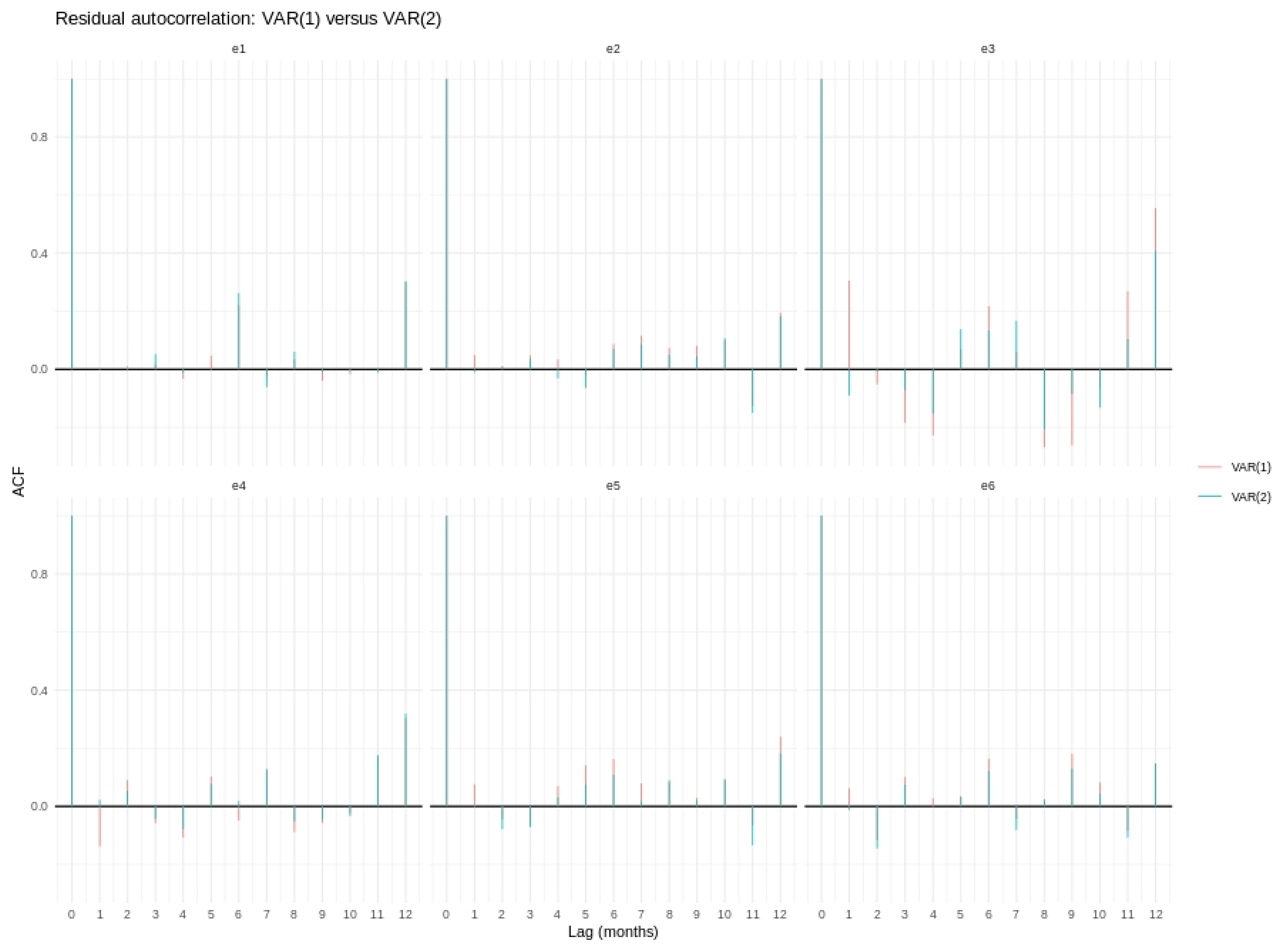
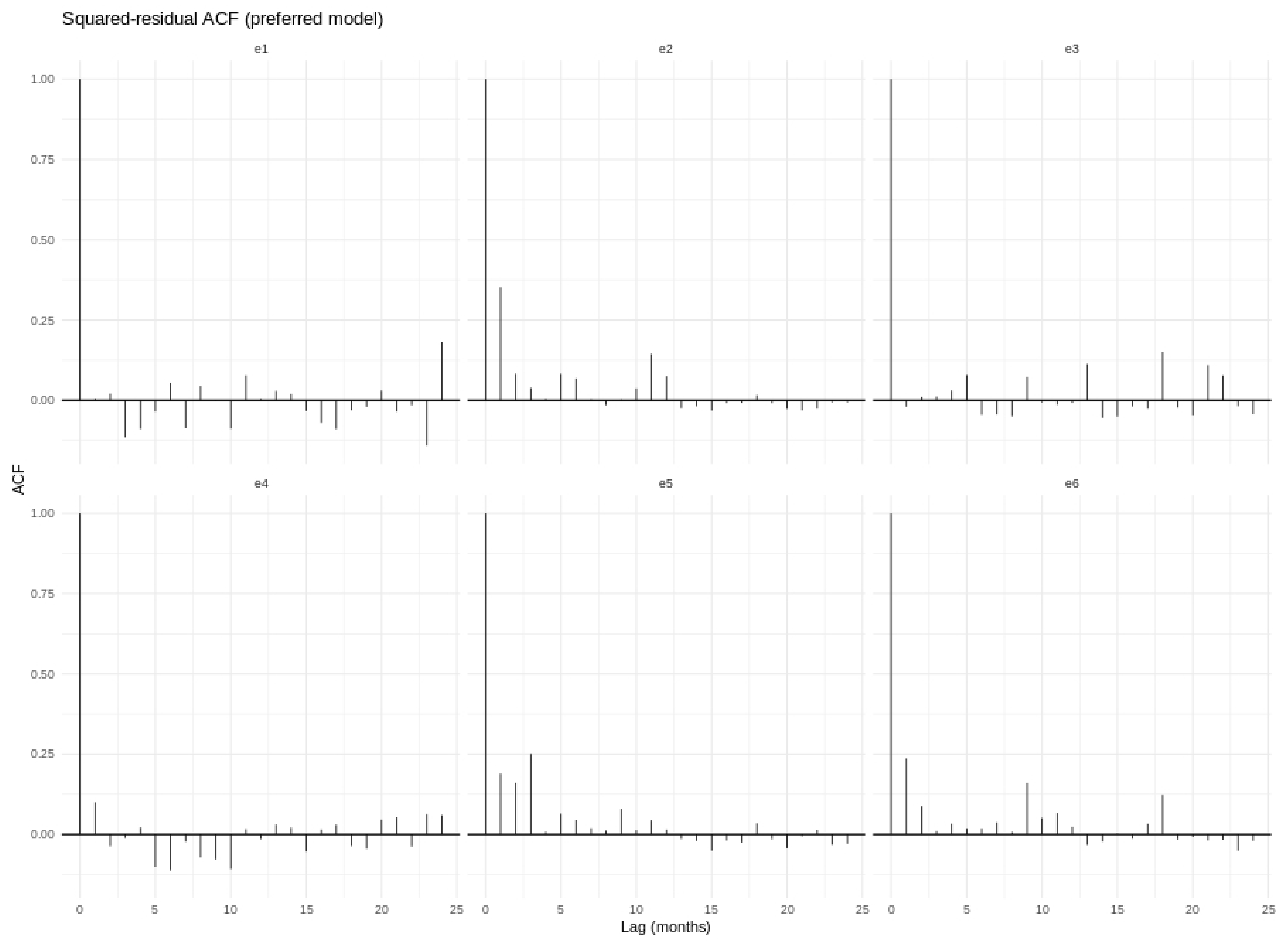
To determine the minimum dynamic order in ALR space, we fitted VAR(1) and VAR(2) models. Figure 4 and Figure 5 compare the coordinatewise residual ACFs from VAR(1) and VAR(2). We applied Ljung–Box and Hosking portmanteau tests to the residuals (

Table 2. Residual diagnostic statistics (lags 1–2 for Ljung–Box, horizon 12 for Hosking portmanteau).

Model	Test	e1	e2	e3	e4	e5	e6
VAR(1)	Ljung–Box p	0.99	0.79	0.00	0.08	0.49	0.20
VAR(2)	Ljung–Box p	0.99	0.98	0.47	0.73	0.57	0.14
Portmanteau ${\chi }^2$/p		628/<0.001 (VAR(2))

). A Ljung–Box residual diagnostic rejects the white-noise null for coordinate $e_3$ under VAR(1) (p < 0.001), whereas no coordinate is rejected under VAR(2) (smallest p-value = 0.14). The residual ACF panels in Figure 4 show that the prominent spikes at lags 1–2 present under VAR(1) vanish when the second lag is added. At the system level, the portmanteau statistic at horizon 12 remains marginally significant; adding centered monthly dummies reduces ${\chi }^2$ from 628 to 431 ($p=0.006$). Because VAR(2) is the smallest specification to clear all short-run autocorrelation and further lags inflate the parameter count without material gain, we adopt a VAR(2) mean and address any residual seasonality through exogenous Fourier terms.

Because the data exhibit markedly different seasonal amplitudes, strong yet uneven cross-correlations, and heterogeneous marginal variability and because residual diagnostics indicate that two lags are the minimum needed for whiteness, we adopt a specification with three complementary elements: a second-order vector autoregressive mean in ALR space to capture short-run dynamics, a single seasonal precision curve common to all components that modulates forecast dispersion across the calendar year, and a Dirichlet observation model that enforces the compositional sum-to-one constraint. Under this Dirichlet layer with a common precision scalar ${\varphi }_t$, componentwise variances differ only through their mean shares—$\mathrm{Var}(y_{t,j}\mid {\mu }_t,{\varphi }_t)={\mu }_{t,j}\left(1-{\mu }_{t,j}\right)/({\varphi }_t+1)$—rather than via component-specific precision processes.

All computations were carried out in R 4.3.2 with Stan 2.33 via the cmdstanr interface [26,27]. Data wrangling, graphics, and tables relied on tidyverse [28], lubridate [29], janitor [30], scales [31], patchwork [32], ggcorrplot [33], GGally [34], and kableExtra [35]. Compositional methods used compositions [36] and the transport package for Aitchison norms [37]. Time series estimation and testing employed vars [38], FinTS [39], and MTS [40].

3. Forecasting Model

Let the monthly renewable energy mix be the $J=7$-component composition

$${\mathbf{y}}_t={\left(y_{t,\mathrm{hyd}},y_{t,\mathrm{geo}},y_{t,\mathrm{sol}},y_{t,\mathrm{win}},y_{t,\mathrm{woo}},y_{t,\mathrm{was}},y_{t,\mathrm{bio}}\right)}^{\top }\in {\mathcal{S}}_7,t=1,\dots ,T.$$

Biofuels ($j^{*}=7$) serve as the reference part in every additive-log-ratio (ALR) transform that follows.

We model ${\mathbf{y}}_t$ as a distributed Dirichlet with a parameter vector that factorizes into a simplex-valued mean ${\mathit{\mu }}_t$ and a positive precision scalar ${\phi }_t$:

$$y_t\mid {\mu }_t,{\varphi }_t\sim \mathrm{Dirichlet}\left({\varphi }_t{\mu }_t\right),{\mu }_t\in {\mathit{S}}_7,{\varphi }_t>0.$$

(2)

Let ${\mathit{\eta }}_t=alr\left({\mathit{\mu }}_t\right)\in {\mathbb{R}}^{J-1}$; for $J=7$, this is a six-vector ${\mathit{\eta }}_t={({\eta }_{t1},\dots ,{\eta }_{t6})}^{\top }$ of log-ratios against biofuels. Its inverse is

$${\mu }_{tj}=\frac{exp\left({\eta }_{tj}\right)}{1+{\sum }_{k=1}^{6}exp\left({\eta }_{tk}\right)}(j\le 6),{\mu }_{t,j^{*}}={\left[1+{\sum }_{k=1}^{6}exp\left({\eta }_{tk}\right)\right]}^{-1}.$$

Calendar variation in forecast dispersion is captured by letting the log-precision depend on an intercept and five Fourier harmonics (ten sine/cosine terms):

$$log{\varphi }_t={\mathbf{f}}_t^{\top }\mathit{\gamma },{\mathbf{f}}_t={(1,{\mathbf{g}}_t^{\top })}^{\top },{\mathbf{g}}_t={\left(sin\frac{2\pi t}{12},cos\frac{2\pi t}{12},\dots ,sin\frac{10\pi t}{12},cos\frac{10\pi t}{12}\right)}^{\top },\mathit{\gamma }\in {\mathbb{R}}^{11}.$$

(3)

Short-run cross-technology interactions are modeled with a second-order vector autoregression process in ALR space:

$${\mathit{\eta }}_t={\mathbf{X}}_t\mathit{\beta }+{\mathbf{A}}_1\left({\mathit{\eta }}_{t-1}-{\mathbf{X}}_{t-1}\mathit{\beta }\right)+{\mathbf{A}}_2\left({\mathit{\eta }}_{t-2}-{\mathbf{X}}_{t-2}\mathit{\beta }\right),{\mathbf{X}}_t=I_{J-1}\otimes {\mathbf{f}}_t^{\top },$$

(4)

where (i) ${\mathbf{A}}_1,{\mathbf{A}}_2\in {\mathbb{R}}^{6\times 6}$ are AR coefficient matrices; (ii) ${\mathbf{X}}_t$ block-replicates the 11-vector ${\mathbf{f}}_t$ across the six ALR coordinates, giving ${\mathbf{X}}_t\in {\mathbb{R}}^{6\times 66}$; and (iii) $\mathit{\beta }\in {\mathbb{R}}^{66}$ contains component-specific regression slopes for the seasonal dummies.

With a scalar precision ${\varphi }_t$, the Dirichlet implies a restricted covariance: $\mathrm{Cov}(y_i,y_j)=-{\mu }_i{\mu }_j/({\varphi }_t+1)$ for $i\ne j$, i.e., negative off-diagonals of fixed shape. Therefore, cross-component co-movement beyond the unit-sum constraint enters through the mean dynamics rather than the observation variance. Extensions include generalized Dirichlet or logistic-normal layers, or alternatively component-specific precisions ${\varphi }_{j,t}$ with regularization; we leave these for future work.

3.1. Geometric Preliminaries and Evaluation Mapping

Let $y_t\in {\mathcal{S}}_7$ denote the share vector and $e_t=alr\left(y_t\right)\in {\mathbb{R}}^6$ its additive log-ratio (ALR) coordinates with biofuels as the reference part; ${alr}^{-1}$ restores shares (see Equation (1)). We model the mean in ALR space (Equation (4)) and obtain predictive draws in share space from the Dirichlet observation layer (Equation (2)). Forecasts are evaluated in two complementary spaces: CRPS in share space for joint sharpness and calibration (Equation (5)), and clr-based RMSE in Aitchison geometry for point accuracy (Equation (6)). Because space choice induces different cross-component dependencies, reporting both clarifies where improvements arise.

Reference-free coordinates. The logistic-normal (sometimes “ALN”) family places a Gaussian law on log-ratio coordinates; the isometric log-ratio (ILR) transform provides orthonormal reference-free coordinates with full metric equivalence on the simp- lex [7,41,42]. This means that the DARMA data models with these three link functions are equivalent provided that the same transformation is applied to the priors. We retain ALR for interpretability and continuity with Equation (1).

Each scalar element of ${\mathbf{A}}_1,{\mathbf{A}}_2,\mathit{\beta }$ and $\mathit{\gamma }$ receives an independent $\mathcal{N}(0,1)$ prior. Posterior inference proceeds via Hamiltonian Monte Carlo (four chains; 500 warm-up and 500 retained iterations per chain) in Stan, yielding 2000 draws that underpin all of the density-forecast evaluations presented later.

3.2. Transform-Space VAR(2) (tVAR(2))

Working in ALR coordinates,

$${\mathit{\eta }}_t={\mathbf{F}}_1{\mathit{\eta }}_{t-1}+{\mathbf{F}}_2{\mathit{\eta }}_{t-2}+{\mathbf{X}}_t\mathit{\delta }+{\mathit{\epsilon }}_t,{\mathit{\epsilon }}_t\sim \mathcal{N}(\mathbf{0},\mathbf{\Sigma }).$$

Parameters $({\mathbf{F}}_1,{\mathbf{F}}_2,\delta ,\mathbf{\Sigma })$ are estimated by ordinary least squares with the same seasonal regressors ${\mathbf{X}}_t$. Multi-step forecasts are generated under the Gaussian innovation assumption and mapped back with ${alr}^{-1}$.

3.3. Additive-Log-Ratio Random Walk (ALR–RW)

A drift-free benchmark sets each future ALR vector equal to the most recent observation: ${\mathit{\eta }}_{t+h\mid t}={\mathit{\eta }}_t.$ Back-transformation yields a single point forecast with zero predictive spread.

3.4. Seasonal Naïve Copy-Last-Year (S-NAIVE)

The seasonal naïve approach copies the composition observed 12 months earlier: ${\mathbf{y}}_{t+h\mid t}={\mathbf{y}}_{t+h-12}.$

These four specifications exploit the same information set but differ in how they propagate seasonality, cross-technology dependence, and uncertainty. Section 4 details the rolling protocol used to compare their point and density-forecast performance.

4. Forecast–Evaluation Protocol

Model comparison follows an expanding–window rolling-origin design that mirrors the workflow used by system operators and energy planners. Let ${\tau }_s$, $s=1,\dots ,S$ denote the final observation included in estimation window s and let H denote the fixed forecast horizon ($H=12$). The first origin is ${\tau }_1=$ 2019-01 and the last origin that still admits a twelve-step look-ahead is ${\tau }_S=$ 2024-01; thus, $S=61$. At origin s, the estimation set is $\{{\mathbf{y}}_t:1\le t\le {\tau }_s\}$ while the verification set comprises $\{{\mathbf{y}}_{{\tau }_s+h}:h=1,\dots ,H\}$.

4.1. Generating Predictive Distributions

All four competitors are evaluated on Monte Carlo samples of equal size $M=2000$ to ensure that scoring rules are comparable.

4.1.1. BDARMA

For every origin s, we retain the M posterior draws ${\left\{{\mathit{\theta }}^{\left(m\right)}\right\}}_{m=1}^M$ returned by the Hamiltonian Monte Carlo sampler. Each draw is propagated through the deterministic state Equation (4) for $h=1:H$ steps, producing the latent mean ${\mathit{\mu }}_{s,h}^{\left(m\right)}$; a single realization ${\mathbf{y}}_{s,h}^{\left(m\right)}\sim \mathrm{Dirichlet}\left({\varphi }_{s,h}^{\left(m\right)}{\mathit{\mu }}_{s,h}^{\left(m\right)}\right)$ is then generated from the observation density (2). The empirical set ${\mathcal{P}}_{s,h}^{\mathrm{BDARMA}}={\left\{{\mathbf{y}}_{s,h}^{\left(m\right)}\right\}}_{m=1}^M$ constitutes the predictive distribution.

4.1.2. tVAR(2)

Let ${\widehat{\mathit{\eta }}}_{s,h}$ and ${\widehat{\mathbf{V}}}_{s,h}$ respectively be the conditional mean and covariance of the Gaussian forecast for the ALR vector at horizon h. We draw ${\mathit{\eta }}_{s,h}^{\left(m\right)}\sim \mathcal{N}({\widehat{\mathit{\eta }}}_{s,h},{\widehat{\mathbf{V}}}_{s,h})$, transform with ${\mathrm{alr}}^{-1}$, and obtain ${\mathcal{P}}_{s,h}^{\mathrm{tVAR}}={\left\{{\mathrm{alr}}^{-1}\left({\mathit{\eta }}_{s,h}^{\left(m\right)}\right)\right\}}_{m=1}^M.$ Multi-step forecasts are generated under the Gaussian-innovation assumption and then mapped back to shares with ${alr}^{-1}$, which preserves unit-sum coherence.

4.1.3. ALR Random Walk (ALR–RW)

The point forecast is the last observed ALR vector ${\mathit{\eta }}_{s,0}$. To give the model a distribution that can be scored with CRPS, we set ${\mathit{\eta }}_{s,h}^{\left(m\right)}={\mathit{\eta }}_{s,0}$ for every m and define ${\mathcal{P}}_{s,h}^{\mathrm{RW}}={\left\{{\mathrm{alr}}^{-1}\left({\mathit{\eta }}_{s,0}\right)\right\}}_{m=1}^M.$ The resulting cloud is degenerate but has the same cardinality M.

4.1.4. Seasonal Naïve (S-NAIVE))

For each horizon h, we copy the composition observed exactly one year earlier, ${\mathbf{y}}_{s-12+h}$. As with the random walk we replicate this deterministic vector M times, ${\mathcal{P}}_{s,h}^{\mathrm{S}–\mathrm{NAIVE}}={\left\{{\mathbf{y}}_{s-12+h}\right\}}_{m=1}^M.$

4.2. Scoring Rules

We denote by ${\mathbf{y}}_{s,h}$ the realized share vector at lead h originating from window s. Two proper scoring rules are applied.

4.2.1. Energy Score (Multivariate CRPS)

Writing ${\parallel \mathbf{a}\parallel }_1={\sum }_{j=1}^7\left|a_j\right|$ for the ${\mathcal{\ell }}_1$ norm, the sample-based energy score (ES; a multivariate generalization of the CRPS) is

$${ES}_{s,h}\left(\mathcal{P}\right)={\displaystyle \frac{1}{M}}\sum _{m=1}^M{∥{\mathbf{y}}_{s,h}^{\left(m\right)}-{\mathbf{y}}_{s,h}∥}_1-{\displaystyle \frac{1}{2M^2}}\sum _{m=1}^M\sum _{m^{\prime }=1}^M{∥{\mathbf{y}}_{s,h}^{\left(m\right)}-{\mathbf{y}}_{s,h}^{\left(m^{\prime }\right)}∥}_1.$$

(5)

We use the ${\mathcal{\ell }}_1$ norm so that units are “share points”; ES remains a strictly proper scoring rule under common norms.

4.2.2. Aitchison Root-Mean-Square Error

Let ${\widehat{\mathit{\mu }}}_{s,h}=M^{-1}{\sum }_m{\mathbf{y}}_{s,h}^{\left(m\right)}$ be the posterior mean. With the centered log-ratio $clr\left(\mathbf{p}\right)=(log{p}_1/g,\dots ,log{p}_7/g)$ and geometric mean $g={\left({\prod }_{j=1}^7{p}_j\right)}^{1/7}$, the point-forecast error is

$${RMSE}_{s,h}={∥clr\left({\mathbf{y}}_{s,h}\right)-clr\left({\widehat{\mathit{\mu }}}_{s,h}\right)∥}_2/\sqrt{7}.$$

(6)

Both (5) and (6) reduce to zero for a perfect forecast.

4.2.3. Interval Diagnostics

For BDARMA, the 5th and 95th sample quantiles define a 90% credible interval for each component. Coverage is tallied over all $(s,h)$ pairs.

4.3. External Baseline and Scoring in Electric-Only Space

A matched evaluation against the vintaged EIA–STEO baseline in the EP-only frame uses the same rolling origins, horizons, and scoring rules; see Supplementary Section S1 for construction and Section S2 for the horizon-by-horizon results (Figures S1 and S2; Tables S1 and S2).

4.4. Fixed-Origin Projection

After the rolling study, a single fixed-origin forecast is produced from the complete estimation window 2010-01–2025-01 (${\tau }^{*}=T$). Future Fourier regressors ${\mathbf{f}}_{T+h}$ are generated deterministically, so the only source of uncertainty is the posterior distribution of model parameters, and for tVAR(2) the Gaussian state noise.

5. Results

5.1. Forecast Accuracy Across Horizons

Table 3. Mean Aitchison RMSE across rolling origins. Boldface marks the lowest error at each horizon.

Horizon	BDARMA	tVAR(2)	S-NAIVE	ALR-RW
1	0.0797	0.0821	0.145	0.114
2	0.0990	0.102	0.145	0.179
3	0.111	0.114	0.145	0.228
4	0.119	0.120	0.146	0.258
5	0.125	0.126	0.148	0.274
6	0.130	0.130	0.149	0.281
7	0.135	0.134	0.148	0.279
8	0.140	0.138	0.148	0.266
9	0.145	0.141	0.148	0.240
10	0.150	0.141	0.147	0.202
11	0.157	0.142	0.147	0.164
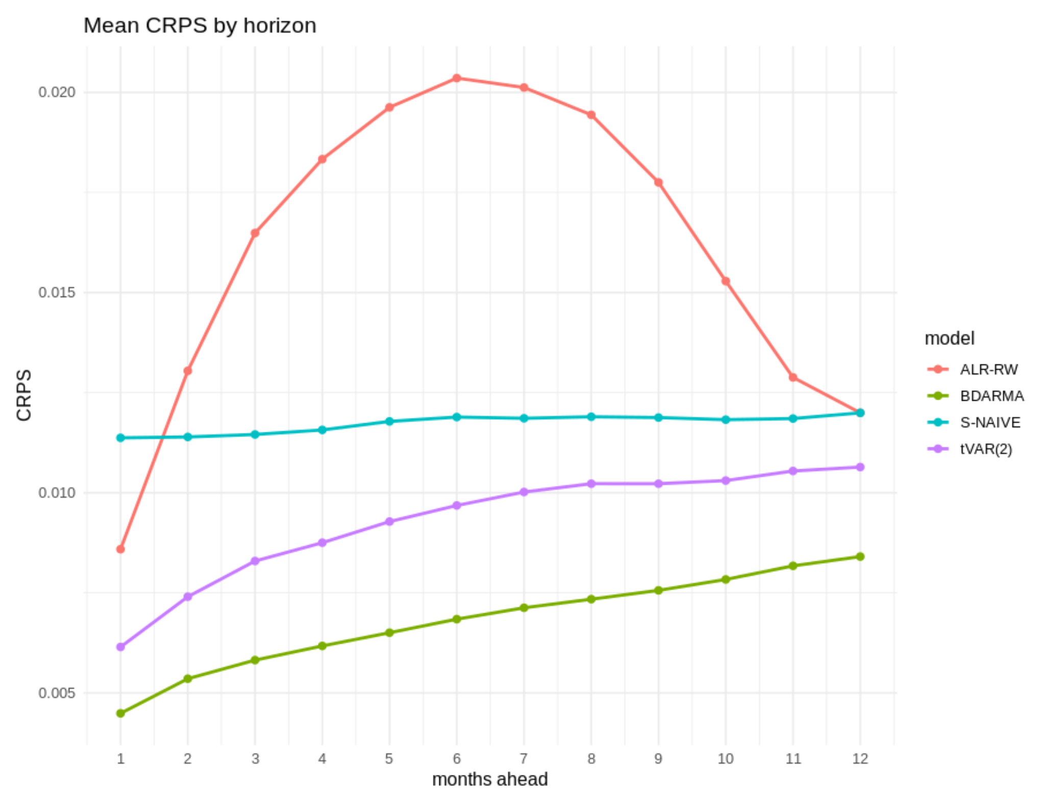
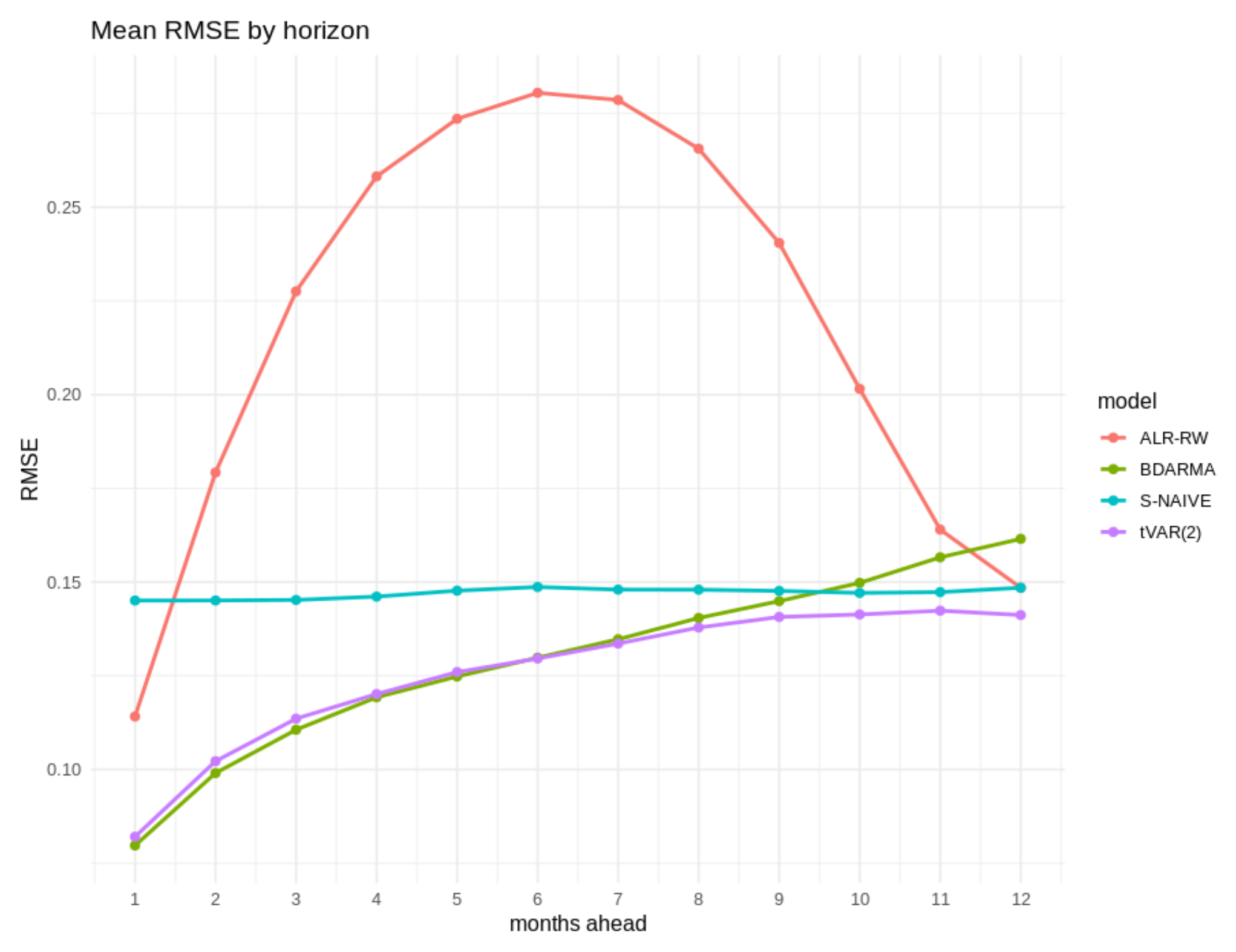
12	0.162	0.141	0.148	0.148

and

Table 4. Mean CRPS across rolling origins. Boldface marks the best score for each horizon.

Horizon	BDARMA	tVAR(2)	S-NAIVE	ALR-RW
1	0.00449	0.00615	0.0114	0.0086
2	0.00535	0.00740	0.0114	0.0130
3	0.00582	0.00829	0.0115	0.0165
4	0.00617	0.00875	0.0116	0.0183
5	0.00650	0.00928	0.0118	0.0196
6	0.00684	0.00968	0.0119	0.0204
7	0.00713	0.0100	0.0119	0.0201
8	0.00734	0.0102	0.0119	0.0194
9	0.00756	0.0102	0.0119	0.0178
10	0.00783	0.0103	0.0118	0.0153
11	0.00817	0.0105	0.0119	0.0129
12	0.00841	0.0106	0.0120	0.0120

report mean CRPS and mean Aitchison RMSE by horizon; Figure 6 and Figure 7 visualize the same quantities. Across sixty-one rolling origins, the Bayesian Dirichlet ARMA (BDARMA) model attains the lowest CRPS at every horizon. At one month, it is about one-quarter lower than the transform-space VAR(2) and more than half lower than either naïve rule, and the advantage widens with lead: by twelve months, BDARMA still improves on tVAR(2) by roughly one-fifth and on S-NAIVE by about forty percent, while ALR-RW remains weakest overall.

Point errors provide a complementary view. Through eight months, BDARMA and tVAR(2) yield nearly identical RMSEs; from month nine onward, the Gaussian VAR gains a small edge that peaks at roughly one hundredth of an Aitchison unit. That edge comes with broader predictive spreads, which shows up as persistently higher CRPS for the VAR.

Technology-Specific Interpretation

Component patterns matter for planning. Wind and hydro exhibit the largest seasonal swings, so their predictive bands are wider and more seasonally structured, informing spring runoff scheduling for hydro and winter ramping reserves for wind. Solar’s long-run rise with a summer plateau produces medium-horizon gains that help to quantify midday surplus risk and storage sizing. Geothermal and waste behave almost deterministically, supporting narrow tolerance bands for compliance or procurement. Wood remains comparatively volatile across horizons, arguing for conservative hedging where biomass supply or policy constraints bind. These qualitative statements align with

Table 5. Componentwise BDARMA coverage (61 by 12 forecasts).

Hydro	Geo	Solar	Wind	Wood	Waste	Bio
0.939	1.000	0.993	0.886	0.954	0.998	0.862

, where geothermal and waste approach perfect inclusion while wind and biofuels are harder to capture due to stronger seasonality and policy or demand variability.

5.2. Coverage of BDARMA Predictive Intervals

The Monte Carlo intervals are well calibrated. Componentwise 90% coverage rises from 86% at one month to 99% by a full year (

Table 6. Empirical 90 percent coverage of BDARMA component intervals.

h	1	2	3	4	5	6	7	8	9	10	11	12
Cov	0.863	0.891	0.907	0.933	0.950	0.957	0.963	0.975	0.984	0.980	0.983	0.985

). By technology (Table 5), geothermal and waste approach perfect inclusion; solar and hydro are very close to nominal; finally, wind and biofuels are lower, consistent with larger seasonal amplitude and policy- or demand-driven swings.

5.3. Fixed-Origin Comparison

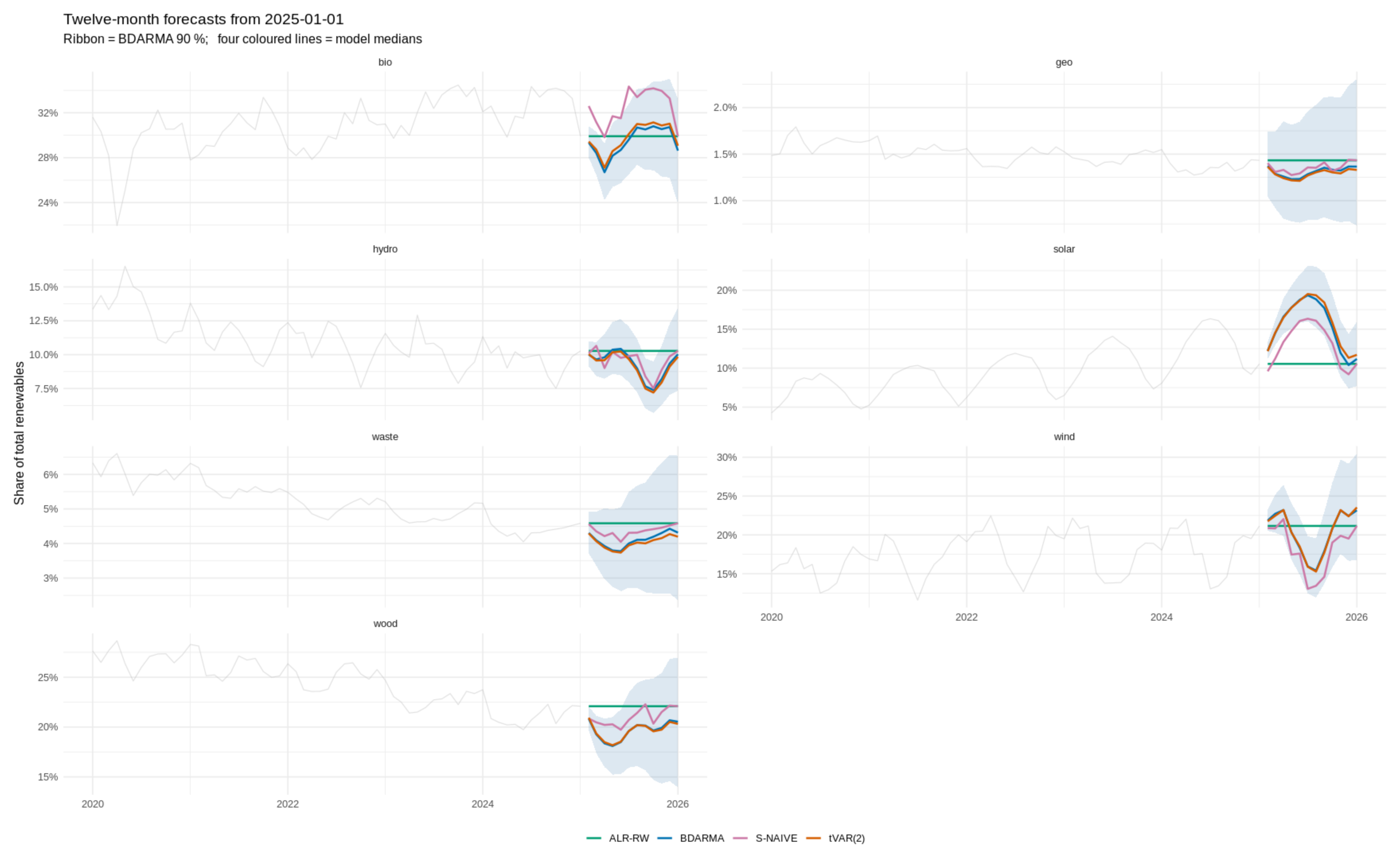
The one-year trajectories in Figure 8 reinforce these patterns. BDARMA produces calibrated bands that widen where seasonality and trend are strong and tighten where series are stable, supporting a single forecast set for both point planning and risk assessment. The naïve rules supply medians only. The Gaussian VAR yields medians close to BDARMA, but cannot indicate whether any remaining gap is material relative to forecast dispersion.

If decisions depend almost entirely on point forecasts, exogenous regressors are abundant and trusted, and speed is critical, then the transform-space VAR(2) is reasonable, especially beyond nine months, where it has a slight RMSE edge. The seasonal naïve approach can suffice for steady components and as a monitoring benchmark where deviations from a baseline are the main signal. BDARMA remains preferable when calibrated densities, compositional coherence, and seasonal uncertainty are central to the decision.

Sequence models such as LSTMs or GRUs can be competitive with long histories and rich covariates. In monthly medium-length settings with few components, they require careful constraints to preserve the unit sum and substantial tuning to obtain calibrated densities. BDARMA offers three practical advantages for this task relative to such sequence learners as well as to gradient-boosted ensembles: (i) coherence by construction (no post hoc renormalization); (ii) direct density forecasts in share space rather than ad hoc bands; and (iii) strong performance with limited history. The approaches are complementary: neural or boosted summaries of weather or policy can enter BDARMA as exogenous features, and neural forecasts can be used as external signals.

Estimation uses four chains with 1000 warm-up and draw counts; origins and chains parallelize across cores. Design matrices grow linearly with the number of components and harmonics.

A matched electric-power-only comparison against the vintaged EIA–STEO baseline confirms the main findings: BDARMA leads at one month, while STEO is strongest beyond two months. Details are in the Supplementary Materials (Sections S1 and S2; Figures S1 and S2; Tables S1 and S2).

6. Conclusions

This paper develops and evaluates a Bayesian Dirichlet ARMA (BDARMA) model for monthly U.S. renewable energy shares, with a VAR(2) mean in additive-log-ratio space and a seasonal Dirichlet precision. In a 61-split rolling evaluation, BDARMA delivers the sharpest and best-calibrated twelve-month density forecasts: mean CRPS is lower than a transform-space VAR(2) at every horizon and far below naïve rules, while point accuracy (Aitchison RMSE) matches the VAR through eight months and stays within roughly two hundredths thereafter. The result is improved uncertainty quantification without sacrificing the central path.

The errors have planning implications by technology. Hydro and wind, our most seasonal components, retain wider seasonally-patterned bands that inform spring runoff scheduling and winter ramping reserves. Solar’s trend plus summer plateau yields medium-horizon gains that tighten estimates of midday surplus risk and storage needs. Geothermal and waste are near-deterministic, justifying narrow tolerance bands, while wood’s broader dispersion argues for conservative procurement where fuel and policy are more volatile.

A balanced view also clarifies when simpler models are reasonable. VAR(2) can be preferred when decisions hinge almost entirely on point forecasts, exogenous regressors are abundant, and computational speed is paramount, while the seasonal naïve approach is defensible for steady systems and as a monitoring baseline. By contrast, BDARMA should be the default when calibrated densities, coherence across components, and explicit seasonality matter for reserves, transmission, and storage planning.

References

- International Energy Agency. Renewables 2024. 2024. Available online: https://www.iea.org/reports/renewables-2024 (accessed on 24 May 2025).
- U.S. Energy Information Administration. Electric Power Monthly, April 2024. 2024. Available online: https://www.eia.gov/electricity/monthly/ (accessed on 24 May 2025).
- U.S. Energy Information Administration. What Is U.S. Electricity Generation by Energy Source? 2025. Available online: https://www.eia.gov/tools/faqs/faq.php?id=427&t=3 (accessed on 1 July 2025).
- Panapakidis, I.P.; Dagoumas, A.S. Day-ahead electricity price forecasting via the adaptive neuro-fuzzy inference system. Energy 2016, 115, 1204–1222. [Google Scholar] [CrossRef]
- Chen, C.; Wang, J.; Hong, T. Short-term load forecasting using the copy-last-day approach with data cleansing. IEEE Trans. Power Syst. 2017, 32, 3536–3537. [Google Scholar]
- Hyndman, R.J.; Athanasopoulos, G. Forecasting: Principles and Practice, 2nd ed.; OTexts: Melbourne, Australia, 2018. [Google Scholar]
- Aitchison, J. The Statistical Analysis of Compositional Data; Chapman & Hall: London, UK, 1986. [Google Scholar]
- Billheimer, D.; Guttorp, P.; Fong, P. Statistical interpretation of species composition. J. Am. Stat. Assoc. 2001, 96, 1205–1214. [Google Scholar] [CrossRef]
- Snyder, R.D.; Ord, J.K.; Beaumont, A. Forecasting the evolution of the age–sex distribution of consumer loans. Int. J. Forecast. 2017, 33, 695–706. [Google Scholar] [CrossRef]
- Zheng, X.; Lin, G.; Chen, J. Dirichlet autoregressive moving average models for compositional time series. J. Stat. Comput. Simul. 2017, 87, 3217–3234. [Google Scholar]
- Koopman, S.J.; Lee, K.; Lucas, A. Dynamic Dirichlet–Multinomial Modelling of Market Shares; Discussion Paper TI 2023-039/III; Tinbergen Institute: Amsterdam, The Netherlands, 2023. [Google Scholar]
- Das, D.; Rangapuram, S.; Benidis, K.; Gasthaus, J.; Salinas, D. Hierarchical Probabilistic Forecasting with Deep Dirichlet Models. In Proceedings of the Proceedings are UAI 2023 (PMLR 216), Pittsburgh, PA, USA, 31 July–4 August 2023; pp. 13327–13335. [Google Scholar]
- Morais, J.; Thomas-Agnan, C.; Simioni, M. Using compositional and Dirichlet models for market share regression. J. Appl. Stat. 2018, 45, 1670–1689. [Google Scholar] [CrossRef]
- Katz, H.; Brusch, K.T.; Weiss, R.E. A Bayesian Dirichlet ARMA model for forecasting lead times. Int. J. Forecast. 2024, 40, 1556–1567. [Google Scholar] [CrossRef]
- Katz, H.; Weiss, R.E. A Bayesian Dirichlet Auto-Regressive Conditional Heteroskedasticity Model for Compositional Time Series. arXiv 2025, arXiv:2507.14132v1. [Google Scholar] [CrossRef]
- Katz, H.; Medina, L.; Weiss, R.E. Sensitivity Analysis of Priors in the Bayesian Dirichlet Auto-Regressive Moving Average Model. Forecasting 2025, 7, 32. [Google Scholar] [CrossRef]
- Wei, Y.; Wang, Z.; Wang, H.; Li, Y. Compositional data techniques for forecasting dynamic change in China’s energy consumption structure by 2020 and 2030. J. Clean. Prod. 2021, 284, 124702. [Google Scholar] [CrossRef]
- He, Y.; Chen, Y.; Zhang, W.; Wang, Y. Optimizing energy consumption structure in Chongqing of China to achieve low-carbon and sustainable development based on compositional data. Sustain. Energy Technol. Assessments 2022, 52, 102340. [Google Scholar] [CrossRef]
- Xu, C.; Xiao, X.; Chen, H. A novel method for forecasting renewable energy consumption structure based on compositional data: Evidence from China, the USA, and Canada. Environ. Dev. Sustain. 2024, 26, 5299–5333. [Google Scholar] [CrossRef]
- Xiao, X.; Li, X. A novel compositional data model for predicting the energy consumption structures of Europe, Japan, and China. Environ. Dev. Sustain. 2023, 25, 11673–11698. [Google Scholar] [CrossRef]
- Qian, W.; Liang, X.; Sun, Y.; Tan, L. A novel adaptive discrete grey prediction model for forecasting development in energy consumption structure—from the perspective of compositional data. Grey Syst. Theory Appl. 2022; Ahead-of-print. [Google Scholar] [CrossRef]
- Zhang, K.; Yin, K.; Yang, W. Predicting bio-energy power-generation structure using a newly developed grey compositional data model: A case study in China. Renew. Energy 2022, 198, 695–711. [Google Scholar] [CrossRef]
- Suo, R.; Wang, Q.; Tan, Y.; Han, Q. An innovative MGM–BPNN–ARIMA model for China’s energy consumption structure forecasting from the perspective of compositional data. Sci. Rep. 2024, 14, 8494. [Google Scholar] [CrossRef]
- Ma, J.; Oppong, A.; Acheampong, K.; Abruquah, L. Forecasting renewable energy consumption under zero assumptions. Sustainability 2018, 10, 576. [Google Scholar] [CrossRef]
- Harris, T.; Devkota, J.; Khanna, V.; Eranki, P.; Landis, A. Logistic growth curve modeling of US energy production and consumption. Renew. Sustain. Energy Rev. 2018, 96, 46–57. [Google Scholar] [CrossRef]
- Goodrich, B.; Gabry, J.; Bürkner, P.; Češnovar, R. rstan: R Interface to Stan, R package version 2.32; R Foundation for Statistical Computing: Vienna, Austria, 2024; Available online: https://CRAN.R-project.org/package=rstan (accessed on 10 September 2025).
- Stan Development Team. Stan Modeling Language Users Guide and Reference Manual, Version 2.33; Stan Development Team (NumFOCUS-sponsored project): Austin, TX, USA, 2023. Available online: https://mc-stan.org/docs/2_33/ (accessed on 10 September 2025).
- Wickham, H.; Averick, M.; Bryan, J.; Chang, W.; McGowan, L.D.; François, R.; Grolemund, G.; Hayes, A.; Henry, L.; Hester, J.; et al. Welcome to the tidyverse. J. Open Source Softw. 2019, 4, 1686. [Google Scholar] [CrossRef]
- Grolemund, G.; Wickham, H. lubridate: Make Dealing with Dates a Little Easier, R package version 1.9.3; R Foundation for Statistical Computing: Vienna, Austria, 2011. Available online: https://CRAN.R-project.org/package=lubridate (accessed on 10 September 2025).
- Firke, S. janitor: Simple Tools for Examining and Cleaning Dirty Data, R package version 2.3.2; R Foundation for Statistical Computing: Vienna, Austria, 2023. Available online: https://CRAN.R-project.org/package=janitor (accessed on 10 September 2025).
- Wickham, H.; Seidel, D. scales: Scale Functions for Visualization, R package version 1.3.0; R Foundation for Statistical Computing: Vienna, Austria, 2019. Available online: https://CRAN.R-project.org/package=scales (accessed on 10 September 2025).
- Pedersen, T.L. patchwork: The Composer of Plots, R package version 1.3.2; R Foundation for Statistical Computing: Vienna, Austria, 2025; Available online: https://CRAN.R-project.org/package=patchwork (accessed on 10 September 2025).
- Kassambara, A. ggcorrplot: Visualization of a Correlation Matrix Using ‘ggplot2’, R package version 0.1.4; R Foundation for Statistical Computing: Vienna, Austria, 2022. Available online: https://CRAN.R-project.org/package=ggcorrplot (accessed on 10 September 2025).
- Schloerke, B.; Cook, D.; Larmarange, J.; Briatte, F.; Marbach, M.; Thoen, E.; Elberg, A.; Toomet, O.; Crowley, J.; Hofmann, H.; et al. GGally: Extension to `ggplot2`, R package version 2.2.0; R Foundation for Statistical Computing: Vienna, Austria, 2021. Available online: https://CRAN.R-project.org/package=GGally (accessed on 10 September 2025).
- Zhu, Z. kableExtra: Construct Complex Table with ‘kable’ and Pipe Syntax, R package version 1.3.4; R Foundation for Statistical Computing: Vienna, Austria, 2021. Available online: https://CRAN.R-project.org/package=kableExtra (accessed on 10 September 2025).
- van den Boogaart, K.G.; Tolosana-Delgado, R. compositions: Compositional Data Analysis, R package version 2.0-8; R Foundation for Statistical Computing: Vienna, Austria, 2024. Available online: https://CRAN.R-project.org/package=compositions (accessed on 10 September 2025).
- Schuhmacher, D.; Heinemann, J.; Schmitz, F. transport: Computation of Optimal Transport Plans and Wasserstein Distances, R package version 0.13-2; R Foundation for Statistical Computing: Vienna, Austria, 2020. Available online: https://CRAN.R-project.org/package=transport (accessed on 10 September 2025).
- Pfaff, B. VAR, SVAR and SVEC Models: Implementation Within R Package vars. J. Stat. Softw. 2008, 27, 1–32. [Google Scholar] [CrossRef]
- Pfaff, B. FinTS: Companion to Tsay (2005) Analysis of Financial Time Series, R package version 0.5-4; R Foundation for Statistical Computing: Vienna, Austria, 2024. Available online: https://CRAN.R-project.org/package=FinTS (accessed on 10 September 2025).
- Tsay, R.S. MTS: All-Purpose Toolkit for Multivariate Time Series Analysis, R package version 1.4.1; R Foundation for Statistical Computing: Vienna, Austria, 2023. Available online: https://CRAN.R-project.org/package=MTS (accessed on 8 September 2025).
- Aitchison, J.; Shen, S.M. Logistic-normal distributions: Some properties and uses. Biometrika 1980, 67, 261–272. [Google Scholar] [CrossRef]
- Egozcue, J.J.; Pawlowsky-Glahn, V.; Mateu-Figueras, G.; Barceló-Vidal, C. Isometric Logratio Transformations for Compositional Data Analysis. Math. Geol. 2003, 35, 279–300. [Google Scholar] [CrossRef]
Figure 1.
Monthly U.S. renewable energy mix, 2010–2025. Hydro loses ground, while wind and solar expand rapidly. Seasonality is most pronounced in hydro (spring runoff) and wind (winter–spring peak). Areas are stacked so each month sums to 100%.
Figure 2.
Seasonal variation in renewable energy shares, 2010–2024. Boxes span the inter-quartile range; black bars mark the median. Means in panel (b) highlight opposing hydro/solar and hydro/wind peaks.
Figure 3.
Cross–source dependence in additive-log-ratio space. Positive (red) and negative (blue) correlations in panel (a) exceed 0.9 in absolute magnitude; scatter plots in panel (b) reflect the nonlinear shape induced by the simplex geometry. *** Indicates the significance level of the correlation coefficient.
Figure 4.
Residual autocorrelation by ALR coordinate: red = VAR(1); blue = VAR(2). Adding the second lag removes the large spikes at lags 1–2.
Figure 5.
ACF of squared residuals for the preferred VAR(2) + season model.
Figure 6.
Mean CRPS by horizon, averaged over 61 rolling origins. Lower values indicate sharper and better-calibrated densities.
Figure 7.
Mean Aitchison RMSE by horizon. Lower values indicate more accurate point forecasts.
Figure 8.
Twelve-month forecasts issued 1 January 2025 after refitting all models to the 2010–2024 sample. Blue shading denotes the BDARMA 90% predictive interval. Colored lines are posterior or plug-in medians. Axes are free by facet.