Multifeature-Driven Multistep Wind Speed Forecasting Using NARXR and Modified VMD Approaches

Abstract

The global demand for clean and sustainable energy has driven the rapid growth of wind power. However, wind farm managers face the challenge of forecasting wind power for efficient power generation and management. Accurate wind speed forecasting (WSF) is vital for predicting wind power; yet, the variability and intermittency of the wind make forecasting wind speeds difficult. Consequently, WSF remains a challenging area of wind research, driving continuous improvement in the field. This study aimed to enhance the optimization of multifeature-driven short multistep WSF. The primary contributions of this research include the integration of ReliefF feature selection (RFFS), a novel approach to variational mode decomposition for multifeature decomposition (NAMD), and a recursive non-linear autoregressive with exogenous inputs (NARXR) neural network. In particular, RFFS aids in identifying meteorological features that significantly influence wind speed variations, thus ensuring the selection of the most impactful features; NAMD improves the accuracy of neural network training on historical data; and NARXR enhances the overall robustness and stability of the wind speed forecasting results. The experimental results demonstrate that the predictive accuracy of the proposed NAMD–NARXR hybrid model surpasses that of the models used for comparison, as evidenced by the forecasting error and statistical metrics. Integrating the strengths of RFFS, NAMD, and NARXR enhanced the forecasting performance of the proposed NAMD–NARXR model, highlighting its potential suitability for applications requiring multifeature-driven short-term multistep WSF.

1. Introduction

The worldwide demand for a clean, green environment and sustainable energy supply has brought about the emergence and tremendous growth of renewable energy technologies, such as those aimed at utilizing wind resources. China, the United States, Germany, and India are some of the leading countries identified with the largest wind capacities. Other countries with significant potential wind resources, including the Philippines, are continuously and enthusiastically paving the way for wind energy installations as the clean energy transition accelerates. However, managing wind farms is a challenge for plant managers and operators in terms of wind power forecasting, which is significant for future energy generation. The wind power produced highly depends on the wind speed, which can by no means be directly influenced through human involvement. To this end, wind speed forecasts are essential for wind farm operators to carry out real-time management through estimating wind power to optimize energy production, maintain grid stability, ensure safety, and plan maintenance activities. Therefore, accurate wind speed forecasting (WSF) is essential; however, the stochastic nature and irregular intermittency of the wind make wind speeds complicated and difficult to forecast. Wind speed estimation is an indispensable component of wind energy production processes, and it is highly essential for it to be quantified accurately; thus, continuous improvements have been made in this regard.

Previous studies have utilized only historical wind speed patterns as input features for WSF models [1]. However, according to [2], meteorological features such as wind direction, temperature, and humidity are considered to make major contributions to the unexpected variations in wind speed. Alongside these factors, the authors of [3] have further suggested that integrating other features, such as atmospheric pressure and air density, will improve WSF. This was further strengthened in [4], where WSF was conducted relying solely on wind speed information as an input. This study revealed that considering the internal relationships between wind speed and other meteorological features may be a promising direction for WSF. Needless to say, it is critical to identify or choose those meteorological factors that provide substantial contributions to the performance of forecasting models while discarding unnecessary factors [5]. In this line, the authors of [6] have emphasized that the identification and inclusion of meteorological features that have significant effects on wind speed may serve as an inherent preprocessing stage in wind speed forecasting. Using multiple uncorrelated input parameters often unfavorably affects the potential of forecasting models [7]. Moreover, a prediction model’s performance is typically degraded as a result of the high dimensionality of the numerous input variables. Feature selection methods evaluate the functional connection between an input variable and a target variable. These methods simplify the process of choosing appropriate inputs for forecasting models, which can considerably improve their performance [8]. The authors of [9] have investigated the significance of feature selection in predictive systems for sustainable energy sources such as marine, solar, and wind energy and revealed that the integration of feature selection enhanced the predictive accuracy in applications related to renewable energy. ReliefF, a filter-style feature selection algorithm, was used to identify key features in meteorological time-series data that served as predictors of wind speeds. This study revealed that ReliefF significantly reduced the complexity of the forecasting model. Gram–Schmidt-based feature selection has also been used to reduce model complexity, allowing the optimal inputs for the model to be chosen while discarding meteorological factors that showed no important contributions to WSF [10]. Sequential feature selection, ReliefF, neighborhood component analysis for regression, and Gaussian process regression have been used as feature selection methods to reduce the dimensionality of inputs [11]. The authors of [12] reviewed various feature selection methods and noted that relief-based algorithms (RBAs) outperformed the alternative methods, with ReliefF being the best and most extensively implemented RBA due to its robustness to noisy data [13].

Previous studies on short-term forecasting have been conducted based on making predictions one step ahead in time, however, the inadequacy of single-step forecasting has been reported, resulting in limitations for wind power system management [14]. Developing and enhancing models that yield acceptable errors as the forecast horizon widens remains a challenge, given the inherently noisy nature of wind data. While performing single-step forecasting of a time-series is a difficult task, predicting multiple steps ahead is undeniably more challenging. Consequently, together with building a model, it is crucial to make parallel efforts in exploring multi-step ahead forecasting strategies. Notable strategies, including recursive, direct, and multiple-input–multiple-output (MIMO) strategies, have been presented to handle this complex problem [15,16]. Comparisons were highlighted, revealing that recursive strategies are seemingly widely used for real time- series.

Alongside the related meteorological factors, the non-linearity and non-stationarity of the wind speed pose a particular challenge for accurate WSF. There is increased interest among researchers in enhancing WSF models through the utilization of hybrid wind time-series analysis for the purpose of extracting effective information from wind time-series data, enhancing the accuracy of WSF [17,18]. Furthermore, it is important to note that, in the recent literature on WSF models integrating signal decomposition approaches, time-frequency analysis was performed on only univariate history observations of wind speed (see, e.g., [4]). These studies did not pay much attention to the fusion of meteorological features that have been demonstrated to have significant impacts on variations in wind speeds. Two of the most widely used decomposition techniques are empirical mode decomposition (EMD) and variational mode decomposition (VMD). The remarkable flexibility and efficiency of EMD—particularly for non-stationary random signals—led to its widespread adoption in the area of signal processing for a variety of applications; however, it suffers from sensitivity to the sampling rate and an inadequate robustness to noise [19]. On the contrary, VMD exhibits robustness to noise and overcomes the mode-mixing problems of EMD. Researchers have recently shown considerable interest in VMD—a non-recursive decomposition method—due to its ability to handle varying sampling frequencies and high frequency resolutions. In order to achieve the adaptive decomposition of time-varying signals, the VMD adaptive signal processing technique iteratively searches for the best solution for each mode, defined in terms of the principal frequency and decomposition window width [20]. It is utilized to break down a real-valued input signal into a collection of band-limited intrinsic mode functions with particular sparsity characteristics while preserving the original input. In the process, VMD splits the signal spectrum by setting the number of modes and transferring the signal decomposition to the frequency domain. Therefore, mode mixing can be successfully prevented throughout the decomposition procedure. However, the utilization of VMD is subject to various restrictions [21,22]. For example, VMD is highly dependent on the number of modes for the decomposition of intermediate frequencies. The number of modes (k) must be preset before the decomposition of a signal by VMD is carried out [21]. This makes determining the modes present in a signal imperative for the successful decomposition of the signal. Simply put, VMD possesses the limitation of needing to provide a predefined number of modes k a priori, and its performance may be degraded if the optimal number is not precisely known [22]. In response to this limitation, enhancements and alternative methods have been used in various real-world applications. For defect detection in complicated rotating machinery, particle swarm optimization was utilized to adaptively choose the parameters through the use of various fitness functions [17]. This approach can track the parameter values well, despite its lengthy operation time and low efficiency. A permutation entropy-based adaptive VMD algorithm has been proposed, and the results indicated that this method can quickly and accurately determine k [23]. In [18], VMD was used in the context of WSF. To determine the exact number of modes, an error analysis was performed for each mode. Based on the analysis results, the optimal mode number was used for variational decomposition. More importantly, although it is effective at decomposing the band-limited intrinsic mode functions (IMFs), VMD has little control over the window frequencies other than the intermediate frequency, which may be essential for preserving the fidelity of the signal. The limitations of VMD are still an open problem; hence, novel solutions for real-world applications are continuously arising [21].

The advent of artificial techniques in recent years has paved the way for the development of various artificial intelligence-based methods for multistep WSF. The literature reveals that neural networks have, indeed, been given much attention and have been widely used for time-series prediction in various real-world applications, due to their adaptable capability to capture non-linear properties reflecting complex patterns such as seasonality [24]. Consequently, various methods using neural networks for multistep-ahead recursive forecasting have been developed. A non-linear autoregressive with exogenous inputs (NARX) network is a recurrent dynamic network that includes feedback connections spanning multiple layers. Such networks are highly effective for modeling non-linear systems, particularly in the domain of time-series analysis [25].

This study aimed to optimize a model for multifeature-driven short-term multistep-ahead WSF, focusing on addressing the shortcomings observed in previous WSF studies. Its main contribution is the integration of (a) ReliefF feature selection (RFFS), (b) a novel approach to VMD for multifeature decomposition (NAMD), and (c) a recursive NARX neural network (NARXR). In particular, the RFFS technique was employed to determine the meteorological features that significantly influence wind speed variations. The need for the NAMD stemmed from the goal of increasing the accuracy of training the neural network on the wind speed and selected meteorological historical data. The NAMD was devised to eliminate the need to pre-define the number of modes in the signal through the use of a novel mode detection method and provide control over the window frequencies adjacent to the principal frequency; hence, NAMD contributes to the idea that, in signal decomposition, the window of the desired frequency has merit in the regeneration of the input signal. This was achieved by utilizing a series of parabolic filters, built in consideration of the window, in order to effectively isolate the required output signals from each other. Further, the NARXR neural network was utilized to improve the overall robustness and stability of the multistep wind speed forecasts.

The remainder of this paper is organized as follows: Section 2 details the proposed model and evaluation method, Section 3 presents experimental results and analysis, Section 4 discusses the findings, and Section 5 provides the conclusion and future research directions.

2. Materials and Methods

2.1. Integration and Workflow

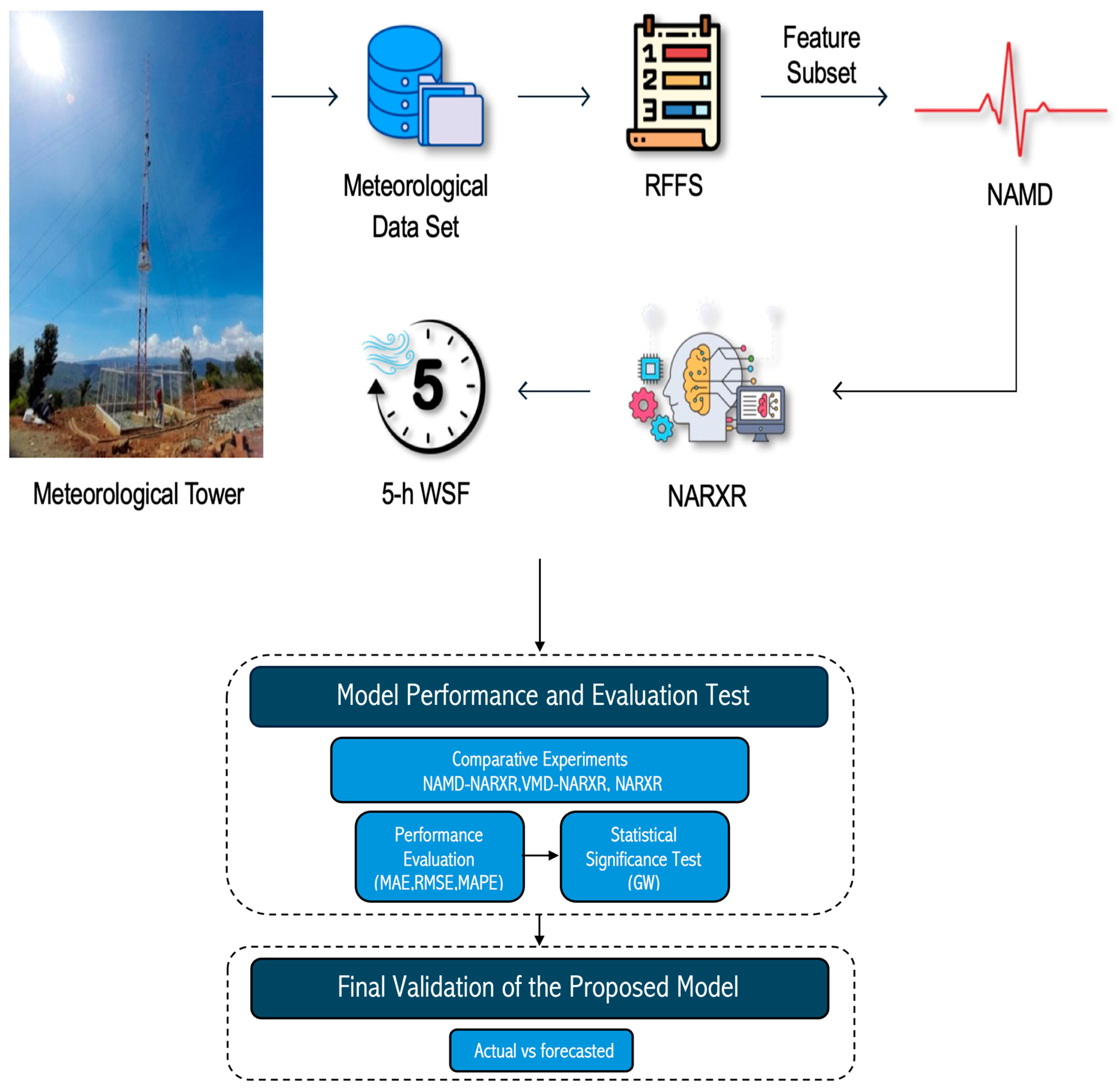
Figure 1 presents the general framework of this study, depicting the three stages that encompassed the development of the proposed 5 h ahead WSF hybrid model; namely, RFFS, the NAMD, and NARXR neural network. Beyond model development, the framework incorporates validation and assessment to ensure forecasting reliability.

2.2. Experimental Data Set

The data set used in this study was obtained from a wind farm in the Philippines, located at 15°49′35.15″ N latitude and 120°11′51.37″ E longitude. This region is representative of a typical wind farm area, benefiting from a favorable wind profile. The location was selected for its dynamic wind conditions and consistent wind flows, which are typical of many wind farms in the region, making it an ideal setting for evaluating the performance of multifeature-driven multistep WSF models. The wind characteristics observed in this area present a realistic challenge for forecasting models, as they must account for significant fluctuations in wind speed over short time intervals.

The data set comprised historical wind speed data obtained from an anemometric sensor positioned at a height of 100 m above ground level, alongside additional sensors measuring meteorological parameters known to have an influence on wind speed variations. These sensors were positioned at various heights on the meteorological tower.

The tower data include historical measurements such as (A) the wind speed (m/s) at 100 m, (B) the relative humidity (%) at 115 m and (C) at 12 m, (D) the wind direction (degrees) at 116 m and (E) at 96 m, (F) the barometric pressure (hPa) at 10 m, (G) the temperature (°C) at 115 m and (H) at 12 m, (I) the air density (kg/m³) at 10 m, and (J) wind gusts (m/s) at 100 m.

All measurements were performed for an observation interval of 10 min and collected from April 2021 to April 2022. The proposed WSF model utilized historical data averaged from 10 min intervals into hourly data to analyze and forecast wind speeds for the subsequent 5 h.

2.3. ReliefF Feature Selection (RFFS)

The performance of any data-driven forecasting model highly depends on the functional associations between the predictor and response variables. According to [12], there is a significant need for feature selection methods that balance computational efficiency with sensitivity to complex patterns of association, such as RBAs. RFFS, recognized as the best and most widely implemented RBA due to its robustness to noisy data [12,13], was used in this study. Specifically, RFFS was employed as a tool for selecting meteorological features that showed significant internal relationships with wind speed.

RFFS randomly chooses an instance $R_i$ and looks for $k$ of its closest neighbors within the same class (known as nearest hits, $H_j$) and from a different class $M_j$(C) (known as nearest misses) [26,27]. The value of k was set to 10, which is generally regarded as suitable for most applications [26]. Parameter $m$ denotes the number of random training instances out of $n$ used to update $W$. A relevance index ($W$) was generated for each feature ($F$), assigning higher weights or scores to features closely associated within the same class and lower weights to closely associated features in other classes. As a result, features that produced the greatest degree of class separation among all of the observations are given a high relevancy index. $W$ can then be used to calculate a complete order of features, eventually ranking each feature according to its relevance when compared with other features. The estimates of the qualities or relevance of the parameters were computed using Equations (1) and (2).

$$W\left(F_n\right)=W\left(F_n\right)-{\displaystyle \frac{{\sum }_{j=1}^{k}diff\left(F_n,R_i,H_j\right)}{mxk}}+{\sum }_{C\ne class\left(R_i\right)}{\displaystyle \frac{\left[\frac{P\left(C\right)}{1-P\left(class\left(R_i\right)\right)}{\sum }_{j=1}^{k}diff\left(F_n,R_i,M_j\left(C\right)\right)\right]}{mxk}},$$

(1)

where the $diff$ function (defined below) determines the difference between values of the features $F_n$ for two instances $R_1$ and $R_2$ of either $H$ or $M$, thus computing the discrepancy between instances to identify the nearest neighbors [26]; n ranges from 1 to 60, representing the total number of features; i ranges from 1 to the total number of samples in the selection data set; the probability of class C is $P\left(C\right)$; and $\mathrm{m}\mathrm{a}\mathrm{x}\left(F\right)$ and $\mathrm{m}\mathrm{i}\mathrm{n}\left(F\right)$ represent the highest and lowest values of feature F across all instances, respectively.

$$diff\left(F,R_1,R_2\right)={\displaystyle \frac{\left|value\left(F,R_1\right)-value(F,R_{2)}\right|}{\max \left(F\right)-\mathrm{m}\mathrm{i}\mathrm{n}\left(F\right)}}$$

(2)

The scores or weights serve as the basis for ranking all meteorological features, and a feature subset can then be established by implementing a threshold criterion to evaluate their relevance. Previous studies initially established the idea of using the maximum distance to the outer line to define the knee point or criteria for the threshold. The knee point concept has been demonstrated to be effective as a reference point in various optimization contexts [27]. Motivated by this concept, a similar threshold criterion was devised utilizing the weights assigned to features. This criterion was used to identify the subset of features chosen from the original set, according to the RFFS ranking. Scores were used to determine the significance of each feature for wind speed. Thereafter, the threshold was determined by identifying the maximum difference between features. In this context, the term ‘difference’ denotes the difference between one feature score and the next. The point where the difference was greatest was determined. Values exceeding this maximum point were deemed to have a minimal impact on wind speed, which led to their eventual exclusion (as in our previous study [6]). In this study, the threshold determination process was enhanced by refining it and applying it iteratively to further streamline the data. This iterative approach was used to identify the subsequent maximum differences, progressively eliminating less-significant features. The process ultimately aimed to reduce the data set to a subset of essential features without compromising the prediction accuracy of the model or losing critical information.

2.4. Novel Approach to VMD for Multifeature Decomposition (NAMD)

Signal decomposition is an important tool which is incorporated to ensure accurate forecasting in real-world applications.

In this study, we propose the NAMD, which leverages a Fourier frequency transform (FFT) for automatic mode detection and employs parabolic filtering to achieve the controlled extraction of signal components, offering a more parametric approach compared to VMD. The need for NAMD stemmed from the goal of increasing the accuracy when training a neural network on historical data. VMD uses the number of modes as a factor when decomposing the intermediate frequencies, where the last decomposed signal of the previous iteration is used for decomposition of the first-mode signal in the next iteration. This makes determining the number of modes k present in the signal imperative for successful decomposition of the signal; consequently, the superior performance of this method may be degraded if the optimal number of modes is not precisely known [22]. Additionally, although effective in decomposing band-limited IMFs, VMD has little control over the window of frequencies beside the principal frequency, which may prove essential in preserving the fidelity of the signal. The proposed NAMD attempts to improve this situation through including the minute nuances and fluctuations referred to as the window frequencies of the principal frequency, thereby improving the neural network’s ability to forecast wind speeds. Generally, NAMD automatically detects the modes in the signal using a mode detection method, then passes the signal to a series of directed parabolic filters that isolate the required signals from each other. This is achieved by taking the output of the mode detector, consisting of the number of modes and frequency points, to create parabolic filters with the size of the window as a divisor for the signal, in order to effectively filter out the principal frequency and its corresponding window components.

Prior to the application of mode detection, the raw signals were prepared to match the required inputs. The preparation of the signal was achieved by first obtaining the FFT of the signal using Equation (3), where $n$ denotes the considered sample, $N$ is the total number of samples, $x_n$ is the time domain signal at index n, ${exp}^{{\displaystyle \frac{-j2\pi }{N}}kn}$ is the complex exponential term with the imaginary unit j, and X_k denotes the FFT output [28]. The resulting signal was shifted such that the zero frequency of the data was situated at the array’s center. This enabled the system to remove the negative components of the FFT. At this point, the signal was ready for mode detection.

$$X_k={\sum }_{n=0}^{N-1}{x}_n{exp}^{{\displaystyle \frac{-j2\pi }{N}}kn}.$$

(3)

The determination of modes and peaks is necessary to obtain a complete decomposition of the original series. In this study, this was accomplished through obtaining the center frequencies provided by the FFT of the signal. The process begins with rectifying the signal such that only positive increments or changes between each data point will be observed. This was obtained using ${\displaystyle \frac{\left(\left|X_{n+1}-X_n\right|+(X_{n+1}-X_n\right))}{2}}$, where a positive change was recorded while negative changes were ignored. The process continued by recording the windowed average of the changes between values, which significantly reduced the variation between the peaks of the desired frequencies. This process is mathematically represented by Equation (4), where $x$ represents the real-valued input points in the sequence, $y$ is the corresponding change in output, $n$ is the length of the signal, and $w$ is the window length (i.e., the number of data points included in the window). This operation yields the windowed positive changes of the signal.

$$y_n={\displaystyle \frac{1}{w-\frac{\left|w-1-n\right|+(w-1-n)}{2}}}{\sum }_{i={\displaystyle \frac{\left|n+1-w\right|+(n+1-w)}{2}}}^n{\displaystyle \frac{\left(\left|X_{n+1}-X_n\right|+(X_{n+1}-X_n\right))}{2}}.$$

(4)

The resulting signal is then passed to a noise reduction phase, where the undesired noise signals are removed to better accentuate the desired peaks. This was achieved by obtaining the maximum and average non-zero values of the signal and shifting the zero point by the average value until the signal satisfied the condition where the average of the non-zero values was greater than or equal to a quarter of the maximum signal. This process is mathematically represented by Equations (5) and (6), where $x_i$ represents data point i, n represents the total number of points in the series, and the function $\mathbf{1}(x_i\ne 0)$ is valued 1 for non-zero values and 0 for zero values, effectively counting only the non-zero values $y$. As a result, the peaks are prominent enough to be detected.

$$y={\displaystyle \frac{\left(\left|x-\frac{\sum _{i=1}^n{x}_i·\mathbf{1}\left(x_i\ne 0\right)}{\sum _{i=1}^n\mathbf{1}\left(x_i\ne 0\right)}\right|+\left(x-\frac{\sum _{i=1}^n{x}_i·\mathbf{1}\left(x_i\ne 0\right)}{{\sum }_{i=1}^n\mathbf{1}\left(x_i\ne 0\right)}\right)\right)}{2}},$$

(5)

$${\displaystyle \frac{\sum _{i=1}^n{x}_i·\mathbf{1}\left(x_i\ne 0\right)}{\sum _{i=1}^n\mathbf{1}\left(x_i\ne 0\right)}}\ge {\displaystyle \frac{{\mathrm{m}\mathrm{a}\mathrm{x}}_{1\le \mathrm{i}\le \mathrm{n}}\left({\mathrm{x}}_{\mathrm{i}}\right)}{4}}.$$

(6)

Subsequently, a signal-thinning method was performed to reduce the peaks to their peak points. This was accomplished by performing forward and reverse increment assessments consecutively—as shown in Equations (4) and (7), respectively—using a single width for the averaging and passing the signal once more to the noise reduction phase mathematically represented by Equation (5). As a result, the output was reduced to the single point value where the peak frequency resided.

$$y_n={\displaystyle \frac{1}{w-\frac{\left|w-1-n\right|+(w-1-n)}{2}}}{\sum }_{i={\displaystyle \frac{\left|n+1-w\right|+(n+1-w)}{2}}}^n{\displaystyle \frac{\left(\left|X_n-X_{n+1}\right|+(X_n-X_{n+1}\right))}{2}}.$$

(7)

The signal was further processed to ensure that the principal frequency was the only peak within the specified window. Essentially, the maximum value in each window of the signal was considered the peak, and all other frequencies within that window were set to 0. This is important as the peaks or modes are detected according to their non-zero values, allowing them to be easily identified and counted by the system. This process identified the number of peaks and the corresponding frequency points in the signals.

The resulting signal was subsequently passed to a filter to isolate the required output signals from each other. In this study, a directed parabolic filter ${(f}_P$) was built in consideration of the window using Equations (8) and (9), which served as a divisor to effectively filter out the principal frequency and its corresponding window components from the signal.

$$f_p=1+{\left({\displaystyle \frac{w_{P_R}-\frac{w_d}{2}}{\frac{w_d}{2}}}\right)}^2,$$

(8)

$$w_{P_R}=\left\{w_P|w_{P_L}\le w_P\le w_{P_U}\right\}.$$

(9)

where $w_{P_R}$ denotes the range of values in the window, $w_P$ refers to the individual values in the window, $w_d$ is the window length, and $w_{P_L}$ and $w_{P_U}$ are the lower and upper components in the window, respectively.

A series of parabolic filters were applied until a specific threshold was reached, defined as the point where the change between the original signal and the filtered output was minimal. The filtered signals were used to recreate the modes by mirroring the positive side of the frequencies to the left, thus recreating the negative points previously removed in the signal preparation phase. The signal was then shifted back to its original position, where the zero-frequency components were to the left of the data array. The resulting signal was used to reconstruct the baseband signal through inverse fast Fourier transform (IFFT) and returned as a series of decomposed signals from the input signal [29].

NAMD was applied to each meteorological feature in the subset.

2.5. Non-Linear Autoregressive Exogenous (NARX) Neural Network

Selecting an appropriate machine learning algorithm is critical for achieving accurate forecasting results. As neural networks possess more complex and adaptable functional structures, they have been effectively used to predict various chaotic time-series. Two types of neural networks have emerged: static and dynamic networks. Static networks have no feedback and derive their outputs straight from the feedforward input they receive. The absence of feedback and memory functions limits the generalization ability of the network, rendering it unsuitable for chaotic time-series forecasting. Alternatively, the outputs of dynamic neural networks are influenced by their input, output, and past and present values in the network structure, making them well-suited for chaotic time-series forecasting [30,31]. A dynamic neural network, known for its strong performance and more effective learning process compared to other neural networks, incorporates feedback links across multiple layers. This network, referred to as the NARX neural network model and described in [11,25,32], was used in this study. 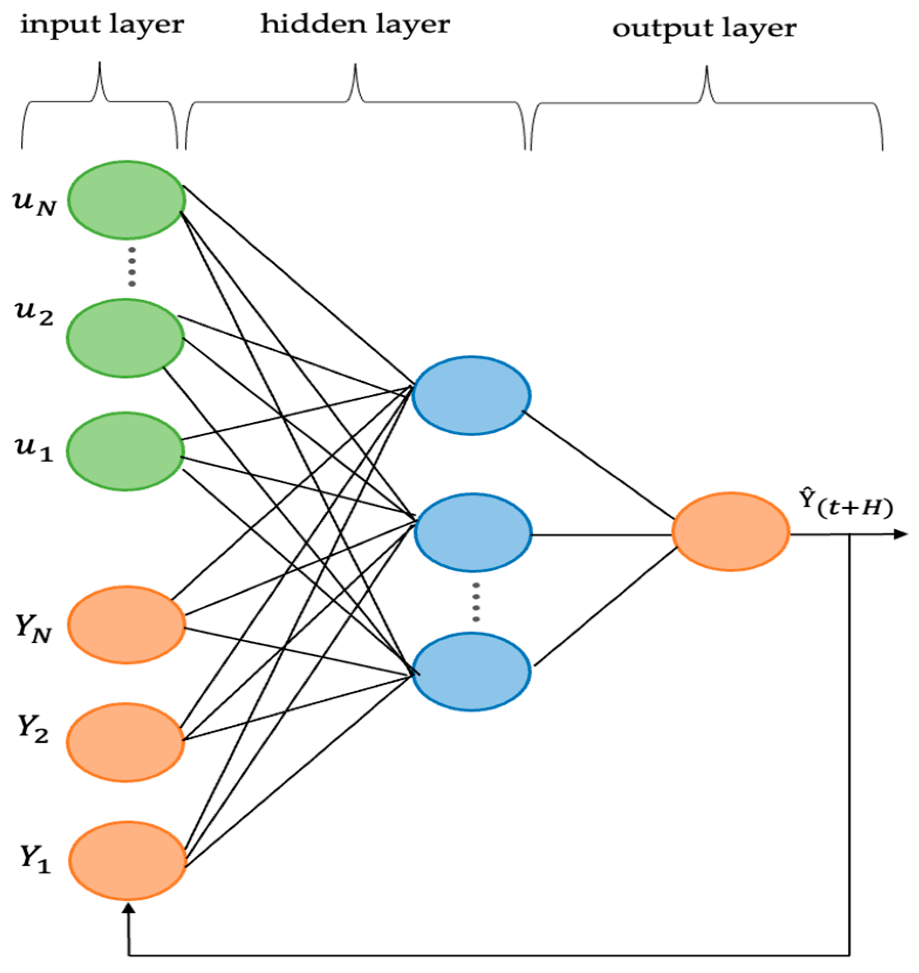In the typical NARX structure detailed in [33,34], the output of the feedforward neural network is looped back and used as an input to the network, as illustrated in Figure 2.

In particular, this study utilized a NARXR in which the model takes the input data and uses the output as part of the input to obtain the next output. The features selected from RFFS were used as the input data. The architecture consists of 4 layers, each containing 500 neurons. The SoftMax function is used as the activation function, while the sparse categorical cross entropy serves as the loss function. The model was trained for 90 epochs. A training-to-testing ratio of 8:2 was used. The training set was used to adjust the model’s parameters, while the testing set was employed to evaluate the model’s performance. The wind and meteorological data were represented as time-series data, with each step denoting an hour. The WSF time-series model was initially trained to conduct single-step forecasting and was eventually applied iteratively for the desired number of steps.

The NARX model input is composed of two parts: the external inputs and the network’s past output, as mathematically represented in Equation (10), where $u_{\left(t\right)}$ represents the external inputs, and $Y_{\left(t\right)}$ denotes the network’s output at time $t$.

$${\mathrm{Ŷ}}_{(t+H)}=f\left(Y_{\left(t-1\right)},Y_{\left(t-2\right)}\cdots Y_{\left(t-N_y\right)},u_{\left(t-1\right)},u_{\left(t-2\right)}\cdots u_{\left(t-N_u\right)}\right).$$

(10)

Furthermore, $f$ is a function that maps the time-series data, ${\mathrm{Ŷ}}_{(t+H)}$ is the wind speed forecast at time $t$ for horizon $H$, and $\left(Y_{(t-1)},Y_{(t-2)},\dots ,u_{\left(t-1\right)},\dots ,u_{(t-N)}\right)$ are the previously observed wind and meteorological time-series data used to forecast the wind speed for the next H hours, where $H$ > 1 represents the absolute forecasting horizon [32,35]. This WSF method is based on the ability to model future wind speeds ($\mathrm{Ŷ}$) as a function of the historical data $Y$ and $u$.

Data from the previous 4 days (consisting of 96 data points) were utilized to forecast the wind speeds in the upcoming hours. For improved accuracy, the first two-step forecasts were predicted by applying the model for $H=1$. Subsequently, the forecast obtained in a given step was included in the input data of the most recent entry for forecasting in the successive step. The entire forecasting horizon was covered by recursively executing this process.

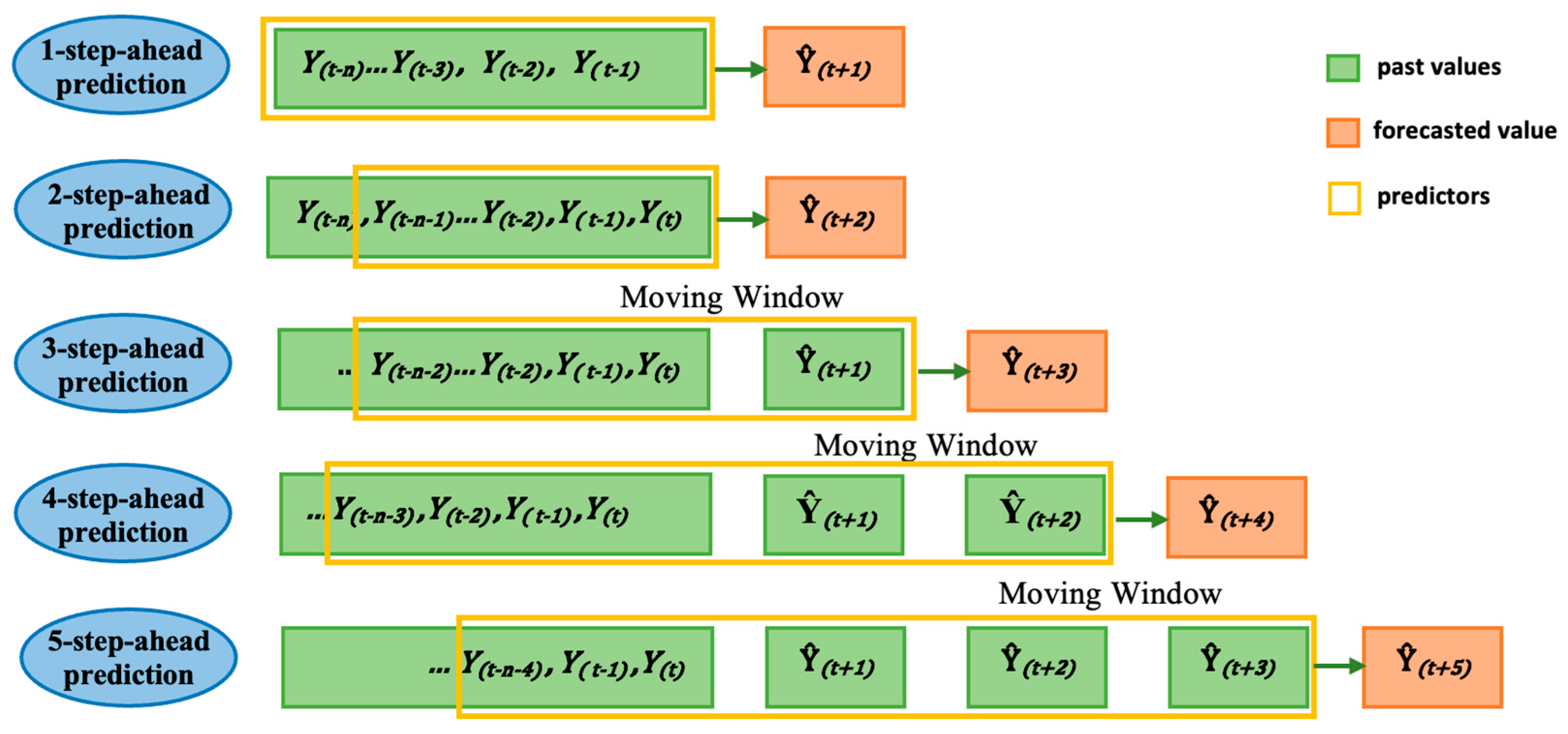
This recursive multistep forecasting mechanism was utilized to create a prediction for the next time step using the resulting forecast in the previous step as part of the input. The design of the multistep prediction model used a recursive architecture, which can be further described using the concept of the sliding or moving window mechanism, as illustrated in Figure 3.

2.6. Performance Evaluation Criteria and Model Comparison

When evaluating the performance of a forecasting model, it is necessary to assess the forecasted values that it produces. In this study, error performance metrics were adopted for this purpose; in particular, the mean absolute error (MAE), root mean square error (RMSE), and mean absolute percentage error (MAPE) were used to quantitatively assess the forecasting performance of the experimental models [4,8,36,37,38]. The measures defined in Equations (11)–(13) indicate deviations between the actual and forecasted wind speed values, where $\mathrm{T}$ denotes the number of prediction samples, $Y_{\left(t\right)}$ denotes the actually observed values at time t, and ${\mathrm{Ŷ}}_{\left(t\right)}$ denotes the predicted values at the same time point. Generally, the performance of a forecasting model improves as these error values decrease.

$$\mathrm{M}\mathrm{A}\mathrm{E}={\displaystyle \frac{1}{\mathrm{T}}}{\sum }_{\mathrm{t}=1}^{\mathrm{T}}|Y_{\left(t\right)}-{\mathrm{Ŷ}}_{\left(t\right)}|,$$

(11)

$$\mathrm{R}\mathrm{M}\mathrm{S}\mathrm{E}=\sqrt{{\displaystyle \frac{1}{\mathrm{T}}}{\sum }_{\mathrm{t}=1}^{\mathrm{T}}{\left|Y_{\left(t\right)}-{\mathrm{Ŷ}}_{\left(t\right)}\right|}^2,}$$

(12)

$$\mathrm{M}\mathrm{A}\mathrm{P}\mathrm{E}={\displaystyle \frac{1}{\mathrm{T}}}{\sum }_{\mathrm{t}=1}^{\mathrm{T}}\left|{\displaystyle \frac{Y_{\left(t\right)}-{\mathrm{Ŷ}}_{\left(t\right)}}{Y_{\left(t\right)}}}\right|\times 100\mathrm{\%}.$$

(13)

To assess the predictive accuracy of the competing forecasting models, we utilize the Giacomini-White (GW) test [39], which examines whether the forecast errors between two models differ significantly. This method compares the absolute errors over an out-of-sample period, as defined in Equation (14), to assess whether the observed differences are statistically significant or merely due to random variation. ${\widehat{e}}_{1t}$ and ${\widehat{e}}_{2t}$ are the forecast errors at time t for models 1 and 2, respectively, $\left(\left|{\widehat{e}}_{1t}\right|-\left|{\widehat{e}}_{2t}\right|\right)$ is the loss differential using absolute errors, $T$ is the total number of forecast errors over the out-of-sample period, and $\widehat{V}$ is the variance–covariance estimate at time t. The authors of [40] further explore the application of this test in forecasting time series, providing additional insights into its usage in real-world scenarios.

$${\widehat{d}}_T={\displaystyle \frac{1}{T}}\sum _{t=1}^T\left(\left|{\widehat{e}}_{1t}\right|-\left|{\widehat{e}}_{2t}\right|\right)\left({\displaystyle \frac{1}{{\widehat{V}}_t}}\right)$$

(14)

The GW test determines whether the difference in forecast errors between the compared models is statistically significant at the 5% level across the different forecast horizons.

The pseudocode shown in Figure 4 outlines the implementation of the proposed NAMD-NARXR model, carried out in Python.

3. Results

3.1. Selection of Significant Meteorological Features

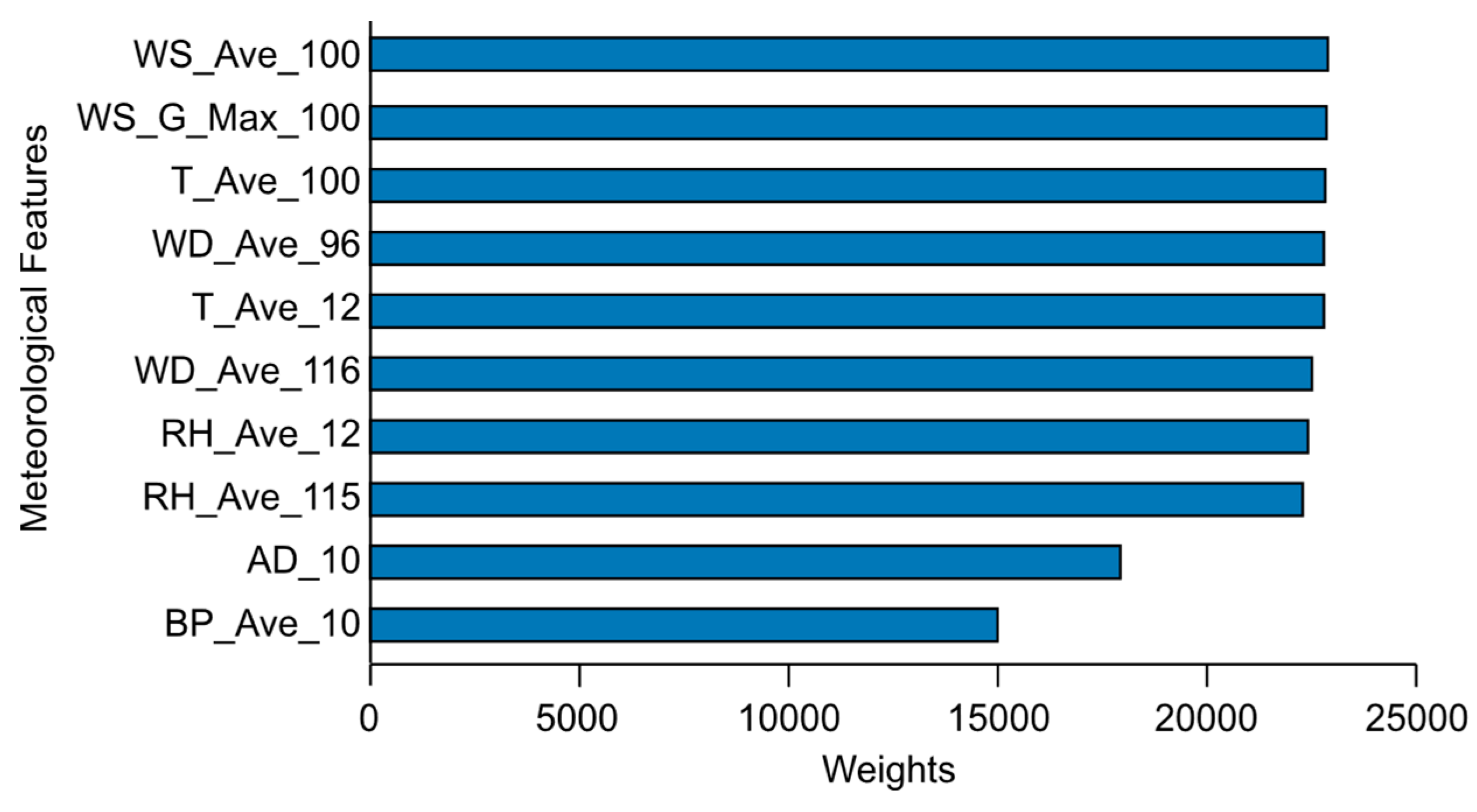
The RFFS process was undertaken to form a feature subset from the experimental data set. A total of 60 features were used to discriminate the 10 base meteorological features. These 60 features correspond to the six recorded values per hour for each of the 10 meteorological features, as data collection was performed every 10 min. Figure 5 presents the ranking of the 10 meteorological features based on their assigned weights. However, only 5 of these meteorological features exceeded the significance threshold and were considered significant for the analysis.

The features were ranked according to their scores or weights, which ranged from 14,834 to 22,876. Figure 5 visually represents the features, ranked in descending order.

Employing the maximum difference between features, the initial threshold criterion or knee point was established. Those features with values equal to or less than this threshold had the least effect on variations in wind speed and, thus, were omitted. To further simplify the data set, the knee point process was repeated once more. Figure 6 depicts the results obtained using the maximum difference between features. This visualization further indicated that all features with scores below 22,758 (marked as Threshold 3 in Figure 6) were regarded as having the least correlation with wind speed. The features demonstrating substantial correlations constituted the feature subset encompassing wind speed, wind gusts, temperature at 115 m, wind direction at 96 m, and temperature at 12 m.

3.2. Descriptive Statistics of the Subset Features

Table 1. Descriptive statistics of the relevant meteorological features.

Meteorological Features	Mean	Standard Deviation	Minimum	Maximum
Wind speed at 100 m	6.232	0.425	0.002	33.760
Wind gusts at 96 m	6.323	0.402	0.228	33.450
Temperature at 115 m	23.159	0.065	17.380	30.900
Wind direction at 96 m	153.653	31.556	0.000	360.00
Temperature at 12 m	23.689	0.072	18.170	31.970

summarizes the descriptive statistics of the relevant meteorological features selected using RFFS. The mean, standard deviation, minimum, and maximum values highlight the variability within the input data, supporting feature selection and enhancing the interpretability of the forecasting model.

3.3. NAMD Results

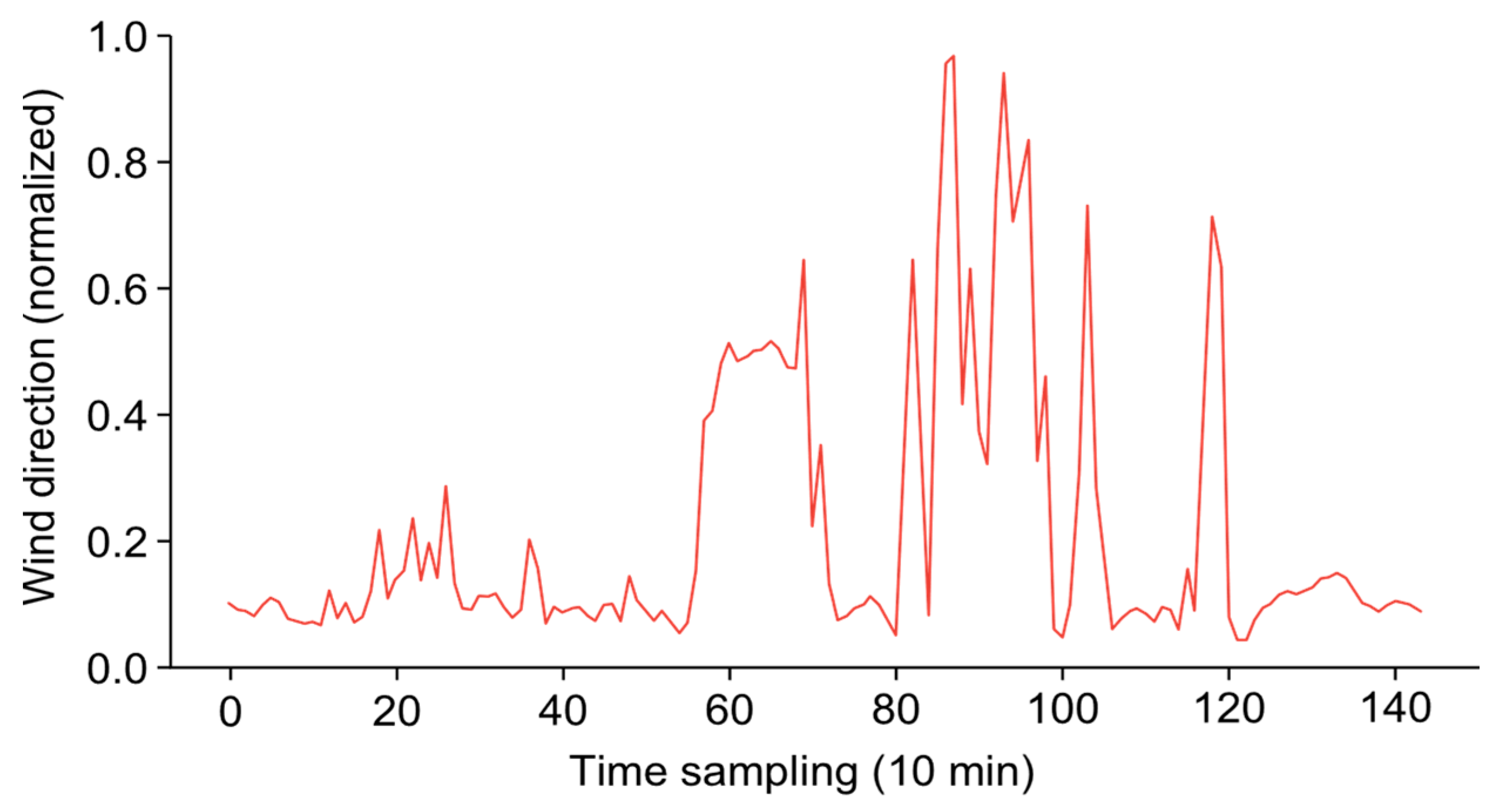
Figure 7, Figure 8 and Figure 9 illustrate the graphical results obtained from the NAMD process. For clarity of discussion and visualization, this study focuses on the wind direction features for a single day, using 144 samples derived from 6 samples per hour.

VMD was unable to intrinsically detect the number of modes in the given signal; hence, k was a priori set to two, in order to extract at least two modes from the IMFs. We took the lower frequency of the IMFs, which is visually reproduced in Figure 9a. This predefined approach can limit the model’s flexibility, particularly when the actual number of modes in the signal is not known or is variable, as it can lead to the decomposition of the signal in a way that does not fully capture the underlying dynamics.

In contrast, NAMD only requires the input of a window, which allows the window frequencies to be retained. The number of modes was automatically detected, with only one mode being identified by NAMD in this particular signal. The IMF returned by the function is shown as a waveform in Figure 9b. The flexibility of NAMD allows it to better capture the true nature of the signal by automatically adjusting to its frequency components. This automatic mode detection is a key advantage, as it ensures the decomposition process is tailored to the structure of the signal, providing more relevant features for forecasting.

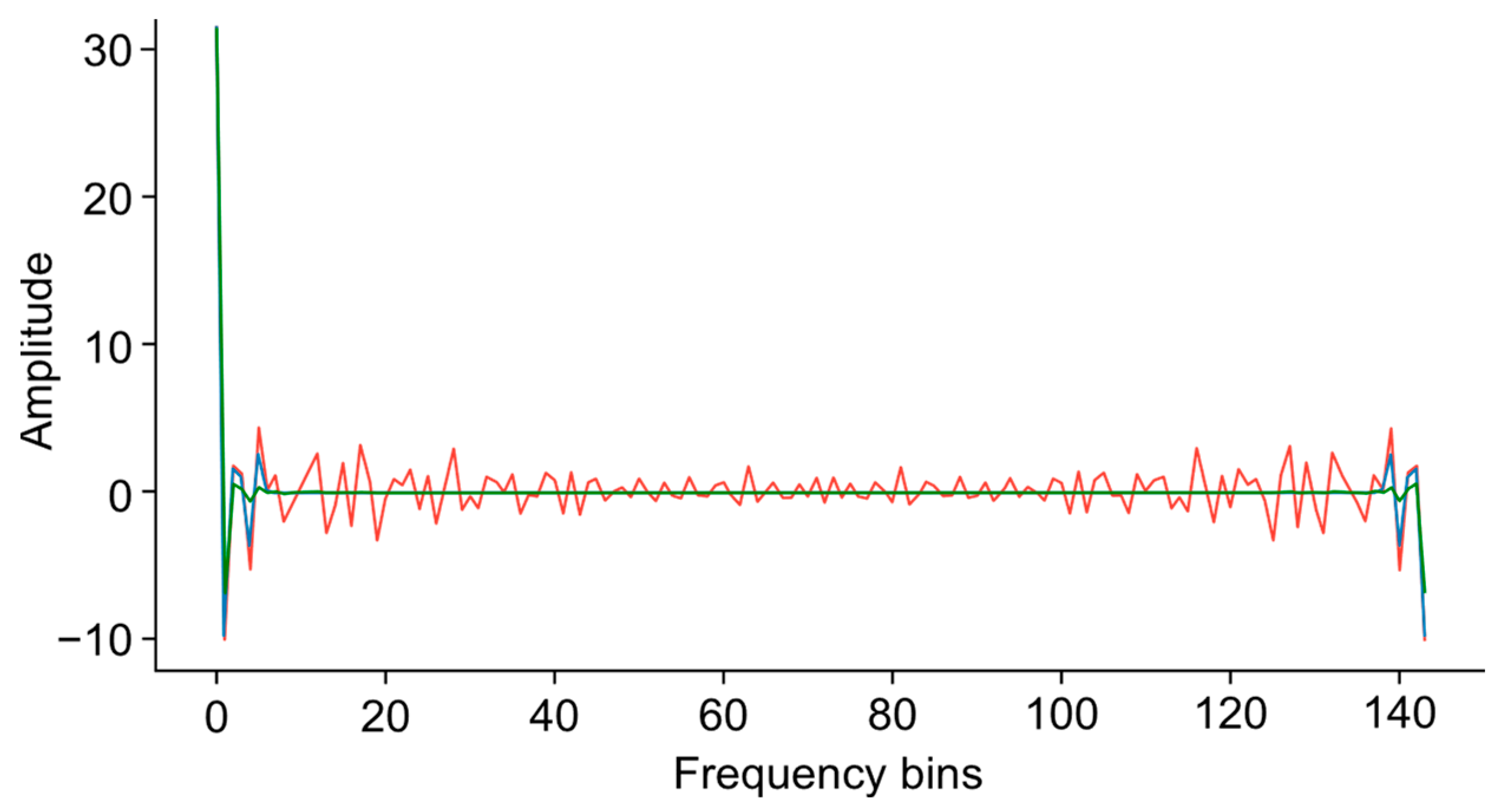
The important distinction between NAMD and VMD is the automatic detection of the number of modes in the signal and the window frequencies allowed. The FFT waveforms generated by both VMD and NAMD may appear similar but, when superimposed against each other, they revealed differences, as shown in Figure 10. VMD generates a frequency spectrum based on the predefined number of modes, which can distort the representation of the actual structure of the signal. On the other hand, the adaptive nature of NAMD ensures a more accurate representation of the frequencies present in the signal. This highlights the importance of automatic mode detection in NAMD, as it allows for a better capture of the true frequency profile of the signal, leading to a more precise decomposition.

Furthermore, the waveforms reconstructed using VMD and NAMD appeared similar but, when compared with the raw data, as shown in Figure 11, they exhibited a significant difference. VMD appears to have filtered out significant information from the raw signal, resulting in a flatter appearance with minimal variances in amplitude. This suggests that the fixed mode decomposition of VMD might have lost important high-frequency components or finer details of the signal.

Meanwhile, the NAMD produced a more precise curve. The reconstructed waveform presented more “windowed” data, maintaining the dynamic characteristics of the signal, making it more representative of the raw data.

3.4. Selection of the Optimal Window Width

Determining the optimal window width is beneficial for preserving the small fluctuations that effectively capture information in a signal, thereby ensuring preservation of the fidelity of the signal. A series of window values were initially tested in order to reveal which value yielded the greatest accuracy. As depicted in

Table 2. Evaluation and selection of the optimal window. MAE, mean absolute error; RMSE, root mean square error; MAPE, mean absolute percentage error.

Window Width	Performance Metrics
	MAE	RMSE	MAPE (%)
5	0.9801	1.4169	16.6456
10	0.9166	1.3792	15.6936
15	0.8143	1.2222	13.7160
25	0.9343	1.3808	15.3924
50	1.0232	1.4921	17.3103
100	1.0468	1.5136	17.7981
200	1.0730	1.6004	17.9594

, the window width of 15 produced the best results across all evaluation criteria, with lower values indicating better performance. Specifically, the MAE of 0.8143 was the lowest error value across all window widths, the RMSE of 1.2222 was the lowest, indicating that the model’s forecasts were closer to the true values, and the MAPE of 13.7160% was the lowest percentage error, suggesting a more accurate forecast. The window width of 15 achieves an optimal balance between retaining sufficient information from the signal and avoiding overfitting, which allows the model to capture essential information without introducing excessive noise or losing important details.

The smaller window widths such as window 5 and window 10 resulted in relatively higher errors across all metrics. Specifically, window 5 had the highest MAE (0.9801) and RMSE (1.4169), while window 10 performed better but still had suboptimal results with MAE (0.9166) and RMSE (1.3792). This suggests that smaller windows failed to capture sufficient frequency components of the signal. By limiting the amount of data used for forecasting, these smaller windows resulted in a less accurate representation of the underlying patterns, leading to higher forecasting errors.

The larger window widths such as window 25 performed relatively well with MAE (0.9343) and RMSE (1.3808) but still had higher error metrics compared to window 15. As the window size increased further (to 50, 100, and 200), the performance began to deteriorate. Window 50 had the highest MAE (1.0232), and the errors continued to increase with larger window widths, with window 200 exhibiting the worst results (MAE = 1.0730, RMSE = 1.6004, MAPE = 17.9594%).

Larger window sizes incorporate more data, but this can lead to overfitting. The model might start to capture unnecessary noise or less relevant data, which distorts the forecasts and increases the error rates. The increased data volume in larger windows could also result in the model becoming too rigid, leading to less flexibility in adapting to the actual characteristics of the signal, thus producing less accurate forecasts.

The optimal window width of 15 achieves the best compromise by effectively balancing data retention and model adaptability. This window width captures enough data to provide meaningful insights into the underlying patterns without overfitting or introducing excessive noise. Both smaller and larger window widths resulted in sub-optimal performance, either by failing to retain enough information or by overfitting to irrelevant data, leading to increased forecasting errors. Consequently, 15 was found to be the optimal window width and was adopted in the NAMD.

3.5. Comparative Accuracy Results for WSF

Comparative experiments were carried out to confirm the performance of the proposed NAMD–NARXR hybrid model in predicting 5-hour-ahead wind speeds in comparison with two models: a VMD–NARXR model and the standard NARXR model. This study focuses on comparing the proposed NAMD–NARXR method with these models, selected for their established use in similar forecasting applications and related time-series problems, as well as their relevance to this study’s objectives. Furthermore, this study aims to address specific limitations of VMD. The inclusion of additional models or hybrid combinations could detract from this focused evaluation by introducing unrelated variables or added complexities. Other models or combinations were not included to maintain a focused comparison and ensure clarity and precision in evaluating the impact of the proposed method.

All selected features obtained from the RFFS were used as inputs to the three models.

3.5.1. Multifeature-Based WSF

As indicated by the experimental results provided in

Table 3. Multifeature-based WSF model performance.

Model	Forecast Step (Hour)	Performance Metrics
		MAE	RMSE	MAPE (%)
VMD–NARXR	1	0.27703	0.75016	5.97178
	2	0.27724	0.75045	5.96606
	3	0.38377	0.92193	8.36465
	4	0.41856	0.97415	9.17157
	5	0.46972	1.07797	10.2739
Proposed NAMD–NARXR	1	0.24777	0.74132	4.78644
	2	0.24788	0.74139	4.78858
	3	0.30468	0.85761	5.76119
	4	0.31089	0.86309	5.81509
	5	0.33169	0.90657	6.31323
Standard NARXR	1	0.27714	0.85354	5.67370
	2	0.27724	0.85354	5.67370
	3	0.30414	0.90355	6.07849
	4	0.31647	0.92980	6.32127
	5	0.33276	0.96642	6.68211

, the proposed NAMD–NARXR model achieved the lowest values across all three error performance metrics for each forecast horizon.

Specifically, for 1-hour-ahead forecasts, the NAMD–NARXR model achieved a MAE of 0.24777, a RMSE of 0.74132, and a MAPE of 4.78644%, outperforming both the VMD–NARXR and standard NARXR models by significant margins.

As the forecast horizon increased to 5 h, the NAMD–NARXR model maintained superior accuracy, with a MAE of 0.33169, a RMSE of 0.90657, and a MAPE of 6.31323%, which were substantially lower than the corresponding metrics of the VMD–NARXR and standard NARXR models.

Compared to the VMD–NARXR model, the NAMD–NARXR model reduced RMSE by up to 38.6%, highlighting its effectiveness in handling multifeature-based WSF.

The results further reveal that the proposed NAMD effectively extracted the principal frequencies and the allowed window frequencies for the wind speed and selected meteorological features. This contributed to its improved performance, particularly for longer forecast horizons, where the decomposition process played a crucial role in capturing complex temporal patterns.

Overall, this clearly demonstrates that the proposed model outperformed the VMD–NARXR and standard NARXR models in terms of predictive accuracy when using all selected meteorological features for wind speed prediction.

3.5.2. Wind Speed-Based WSF

Additionally, the predictive performance of the proposed NAMD–NARXR model was validated using only wind speed as an input. The results provided in

Table 4. Wind speed-based WSF model performance.

Model	Forecast Step (Hour)	Performance Metrics
		MAE	RMSE	MAPE (%)
VMD–NARXR	1	0.27981	0.84134	5.84226
	2	0.27971	0.84127	5.84073
	3	0.32751	0.92373	6.62215
	4	0.34326	0.95471	6.77181
	5	0.35580	0.96936	7.10802
Proposed NAMD–NARXR	1	0.27113	0.82090	5.60708
	2	0.27124	0.82096	5.60922
	3	0.31604	0.91387	6.42729
	4	0.33479	0.95083	6.80876
	5	0.34594	0.97487	7.05190
Standard NARXR	1	0.29675	0.88806	6.13177
	2	0.29696	0.88830	6.13546
	3	0.33661	0.95437	6.71771
	4	0.35441	0.97909	7.03361
	5	0.38516	1.03336	7.61475

highlight the superior performance of the proposed model compared to the benchmark VMD–NARXR and standard NARXR models.

For 1-hour-ahead forecasts, the proposed NAMD–NARXR model achieved a MAE of 0.27113, a RMSE of 0.82090, and a MAPE of 5.60708%, reflecting a reduction in error compared to both VMD–NARXR and standard NARXR models.

Across all forecast horizons, the NAMD–NARXR model consistently outperformed the benchmark models, with an average improvement of up to 3.1% in MAE and 2.4% in RMSE over VMD–NARXR. Compared to the standard NARXR model, the improvements were even more significant, with reductions of 8.6% in MAE, 7.6% in RMSE, and 7.6% in MAPE at the 5-h horizon.

The results confirm the significance of integrating signal decomposition as a preprocessing technique, as evidenced by the comparatively higher error metrics of the standard NARX model. Furthermore, the superior performance of the NAMD–NARXR model over VMD–NARXR highlights the effectiveness of the proposed NAMD method in accurately decomposing raw wind speed signals.

The improved performance of the NAMD–NARXR model can be attributed to the proposed NAMD method’s ability to integrate window frequencies, which enhanced the decomposition process and provided a more robust representation of the wind speed signal. This was reflected in the consistently lower values across all three error performance indicators for every forecast horizon.

In summary, the findings presented in Table 3 and Table 4 validate that the proposed NAMD method performed comparably to VMD in terms of decomposition.

3.6. Comparative Statistical Results for WSF

To further evaluate the overall predictive performance of NAMD–NARXR compared to VMD-NARXR and NAMD–NARXR compared to NARXR, the GW test was applied to the aggregated forecast errors across all forecast horizons. This test allows the determination of whether the observed improvements in performance, as indicated by lower MAE, RMSE, and MAPE, are statistically significant across the different forecast horizons. The multifeature-based WSF test yielded a test statistic of −18.746 with an extremely small p-value of <0.001 and −18.931 with a p-value of <0.001, respectively. In contrast, the wind speed-based WSF test produced a test statistic of −19.226 with an extremely small p-value of <0.001 and −22.359 with a p-value of <0.001, respectively. These results provide strong statistical evidence to reject the null hypothesis of equal predictive ability between the two models. The highly negative test statistic confirms that NAMD–NARXR consistently exhibits lower forecast errors compared to VMD–NARXR and NARXR, further reinforcing its superior predictive performance.

The GW test accounts for the time-dependent nature of errors in the recursive multistep forecasting used, providing a more rigorous comparison between the comparative models. Results for each model comparison for each input type are presented in

Table 5. Statistical comparison of WSF model performance.

Model Input Type	Model Comparison	Test Statistic	p-Value
Multifeature-based WSF	Proposed NAMD–NARXR vs. VMD–NARXR	−18.746	<0.001
	Proposed NAMD–NARXR vs. NARXR	−18.931	<0.001
Wind speed-based WSF	Proposed NAMD–NARXR vs. VMD–NARXR	−19.226	<0.001
	Proposed NAMD–NARXR vs. NARXR	−22.359	<0.001

.

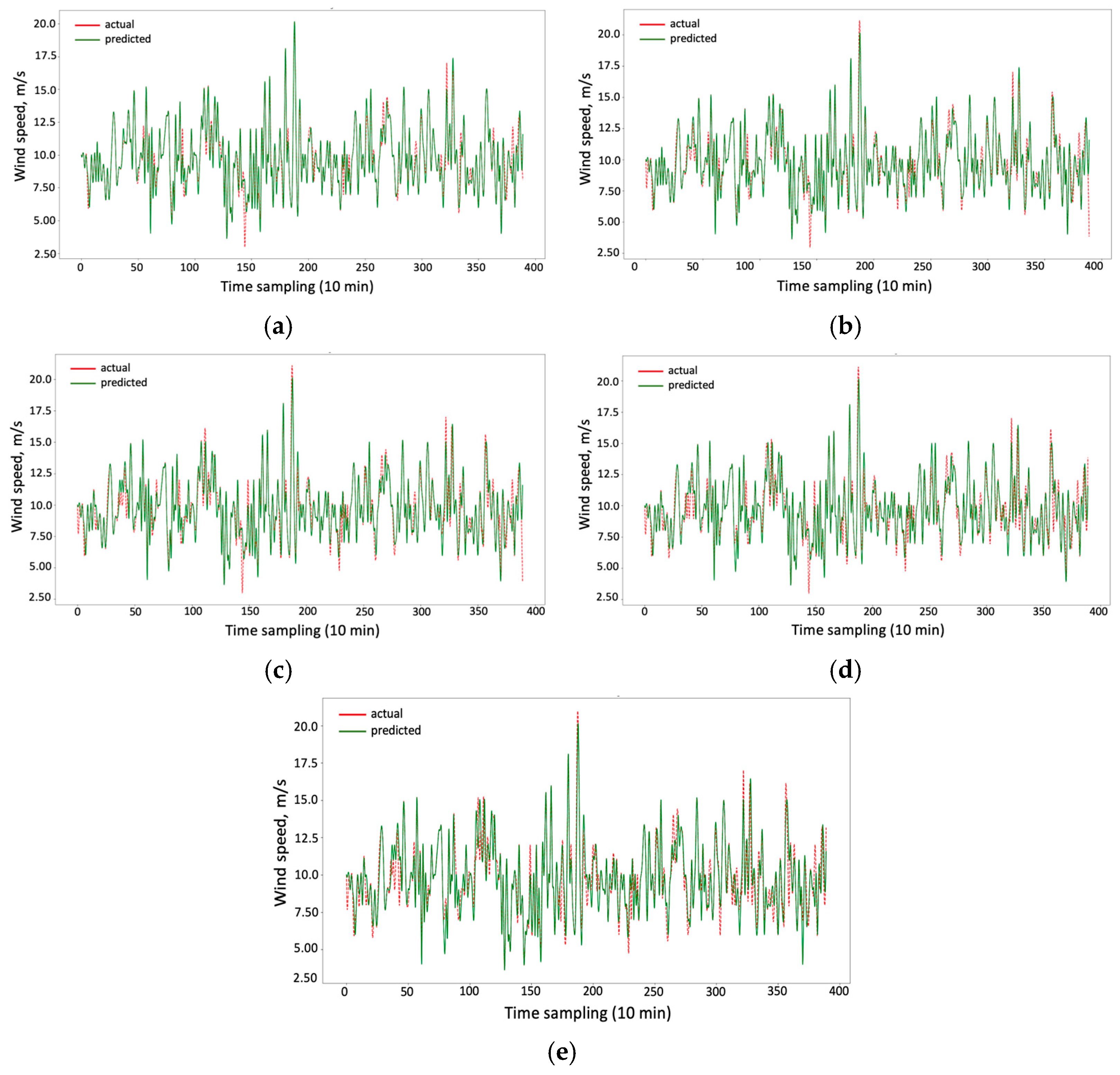
Figure 12 presents out-of-sample forecasts, providing a visual comparison between the forecasted wind speeds produced by the proposed NAMD–NARXR model and the actual recorded wind speeds. As illustrated, at most points in the time-series, the forecasted wind speeds closely matched the actual wind speed trends in all of the forecast horizons, thus confirming the strong predictive performance of the proposed NAMD–NARXR model.

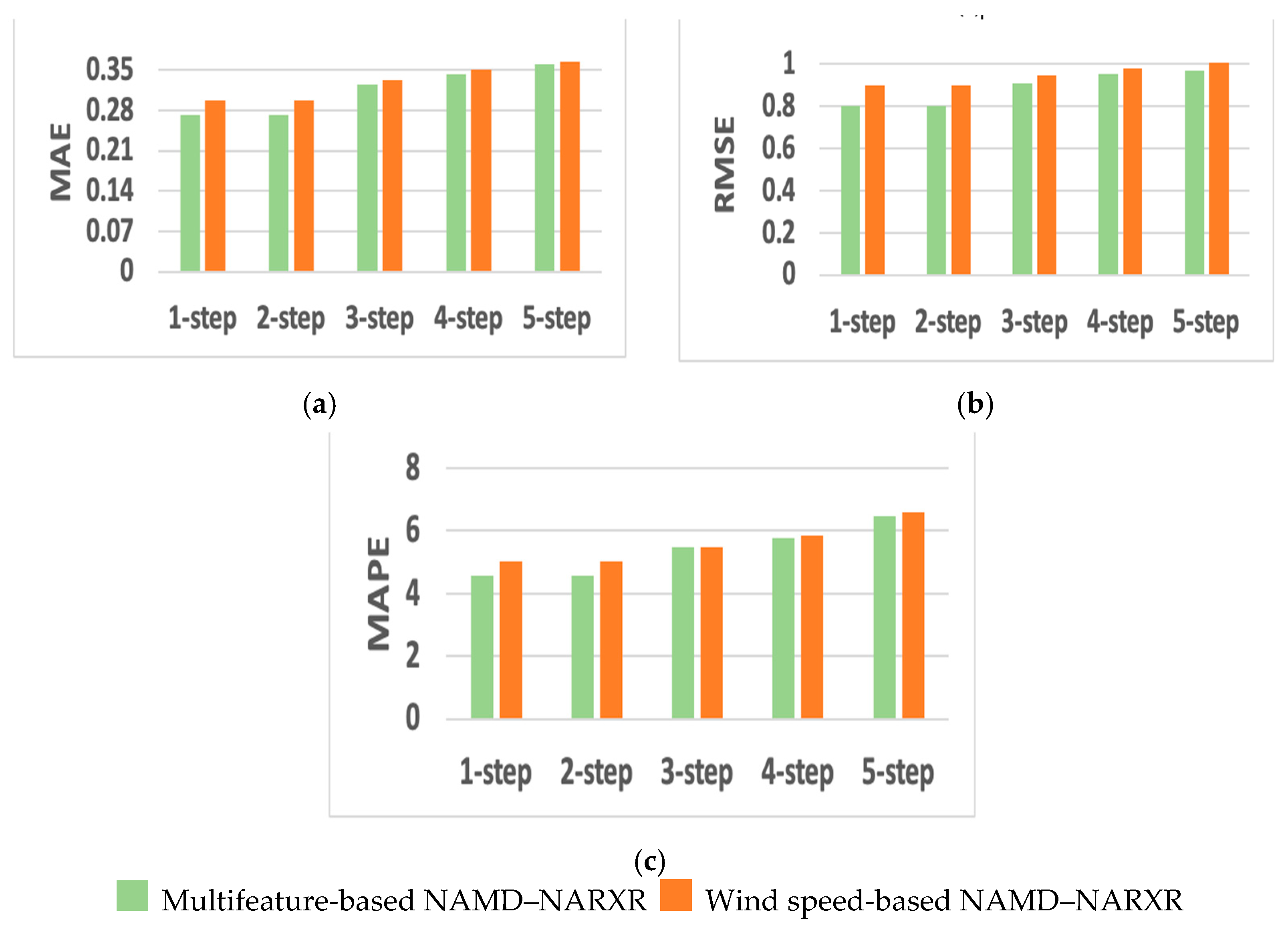
The impact of relying solely on historical wind speed patterns as a predictor of variations in wind speed was compared with the use of historical patterns of the various selected meteorological features. Figure 13 proves that the forecasting accuracy remained consistently higher—as indicated by the lower performance metric values across all forecast horizons—when meteorological features significantly correlated with wind speeds were used as predictors in the forecasting model.

4. Discussion

The results of this study highlight the effectiveness of the proposed NAMD–NARXR method in addressing key limitations of VMD and improving WSF accuracy. The findings can be discussed across three major aspects: feature selection, signal decomposition, and comparative forecasting performance.

The RFFS process demonstrated its capability in identifying significant meteorological features through feature weights, which are critical for accurate WSF. By iteratively applying the maximum difference approach, a concise yet impactful subset of features—including wind speed, wind gusts, temperature at 115 m and 12 m altitudes, and wind direction—was identified. This subset effectively reduced the computational complexity while preserving the predictive relevance of the data, a crucial aspect for real-time applications. The identified features align with known meteorological factors influencing wind dynamics, reinforcing the robustness of the selection process.

The NAMD method demonstrated several advantages over VMD. Unlike VMD, which required a predefined number of modes (k), NAMD automatically detected the number of modes, thereby eliminating the need for a priori assumptions. For instance, in analyzing wind direction signals, NAMD identified only one mode, reflecting the intrinsic characteristics of the signal, while VMD required manual adjustment. The preservation of signal fidelity by NAMD was evident in the reconstructed waveforms (Figure 10), where the NAMD output closely resembled the raw signal, retaining significant information lost in the VMD decomposition. The use of optimal window widths, such as 15, further enhanced the accuracy of NAMD by preserving minute nuances crucial for WSF.

The comparative experiments established the superiority of the proposed NAMD–NARXR model over the VMD–NARXR and standard NARXR models. For multifeature-based forecasting, the NAMD–NARXR model consistently achieved the lowest error metrics (MAE, RMSE, and MAPE) across all forecast horizons (Table 3). This improvement can be attributed to NAMD’s ability to retain principal frequencies and relevant window frequencies, enhancing the quality of inputs to the NARXR model.

When using only wind speed as an input, the NAMD–NARXR model continued to outperform the benchmark models (Table 4), further validating the effectiveness of the NAMD decomposition. These results underscore the importance of integrating advanced signal decomposition methods like NAMD as preprocessing steps in forecasting frameworks.

Furthermore, the results in Figure 13 demonstrate the impact of incorporating multiple meteorological features into the forecasting model. The comparative graphs show that the multifeature-based NAMD–NARXR model consistently achieved lower MAE, RMSE, and MAPE values across all forecast horizons compared to the wind speed-based NAMD–NARXR model. This highlights the limitations of relying solely on historical wind speed patterns and the advantages of leveraging additional meteorological variables to enhance predictive performance.

The superior performance of the multifeature-based model can be attributed to its ability to capture complex dependencies between meteorological factors and wind speed variations. Wind speed is influenced by multiple atmospheric conditions, including wind gusts, temperature, and wind direction, which contribute valuable predictive information beyond historical wind speed alone. By leveraging these additional inputs, the model effectively reduces forecast uncertainty, leading to more reliable short-term wind speed predictions.

These findings align with prior studies that have emphasized the importance of multifeature-driven forecasting approaches. The consistent reduction in forecast error across all steps further underscores the robustness of the selected features.

The GW test results indicate a statistically significant improvement in predictive accuracy when using NAMD–NARXR over VMD–NARXR and NAMD–NARXR over NARXR. A statistically significant result (i.e., p-value < 0.05) indicates that one model outperforms the other in terms of forecast accuracy. The test statistic values in Table 5 suggest that, across all forecast steps, the forecast errors of NAMD–NARXR are consistently lower than those of VMD–NARXR and NARXR. The extremely small p-values suggest that the probability of obtaining such a large test statistic under the assumption of equal predictive ability is negligible, confirming that the observed performance difference is not due to random chance.

Instead of applying the GW test separately for each forecast step, we evaluated the overall model performance by aggregating the forecast errors across all horizons. This approach provides a more comprehensive assessment of the models’ predictive ability, ensuring that performance differences are not limited to a specific forecast horizon but hold across the entire forecasting range.

The GW results further emphasize the importance of evaluating forecasting models using statistical tests that account for time-dependent error structures, particularly in recursive multistep forecasting, where forecast errors propagate over time. The superiority of NAMD–NARXR over both alternatives highlights its effectiveness in capturing the underlying patterns of wind speed variations more accurately.

5. Conclusions

This study advances the field of wind speed forecasting by introducing a novel approach to signal decomposition, specifically the NAMD method, and applying it to short-term multistep wind speed forecasting. By addressing the limitations of traditional methods, such as VMD, we provide a more flexible and robust alternative that enhances forecasting accuracy, especially in the context of complex, real-world applications.

The findings of this research demonstrate the potential of NAMD to effectively decompose meteorological data and improve the performance of forecasting models, notably the proposed NAMD–NARXR. Additionally, the integration of RFFS ensures that only the most relevant meteorological predictors are utilized, further enhancing forecasting accuracy. By comparing it to existing methods, we show that the proposed model offers improved prediction accuracy across multiple forecasting horizons, which is critical for the operational use of wind speed forecasts in the Philippine setting and other regions with similar complexities.

Importantly, this study addresses a significant gap identified in the introduction: the need for better signal decomposition techniques that automatically determine the number of modes and incorporate window frequencies in the decomposition to handle the complexity of real-world wind speed data. Our findings highlight that improving decomposition techniques can lead to more accurate and reliable wind speed predictions, which can contribute to better energy management and decision-making in renewable energy systems.

In conclusion, our work offers a meaningful contribution to the field of wind speed forecasting by not only providing a novel method but also setting the stage for further research that can enhance the application of forecasting models in renewable energy systems. The potential for improving forecasting accuracy through better signal processing holds considerable promise for researchers in the field.

While this study demonstrates the effectiveness of NAMD–NARXR, further research could enhance its applicability. Exploring adaptive techniques for window width selection may improve flexibility across varying signal characteristics. Additionally, integrating NAMD with other forecasting models could expand its versatility, while comparing it with alternative denoising methods (e.g., Wavelet Decomposition, Ensemble Empirical Mode Decomposition) may offer deeper insights into its relative performance.

Future studies could also evaluate NAMD–NARXR against additional forecasting models or hybrid approaches to further assess its predictive capabilities. Incorporating additional evaluation metrics would provide a more comprehensive performance assessment. Moreover, validating the model across different seasons and diverse wind farms in the Philippines—considering various geographical and climatic conditions—would help ensure its robustness, adaptability, and real-world applicability.