

Forecasting Wind Speed Using Climate Variables


Abstract
1. Introduction
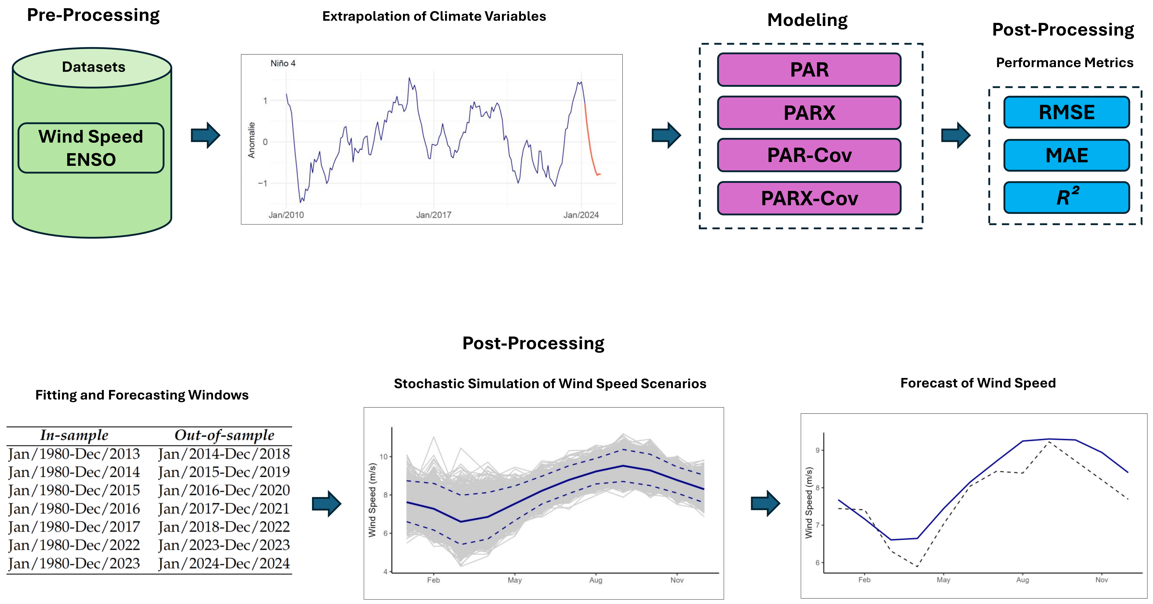
2. Methodology
2.1. Pre-Processing
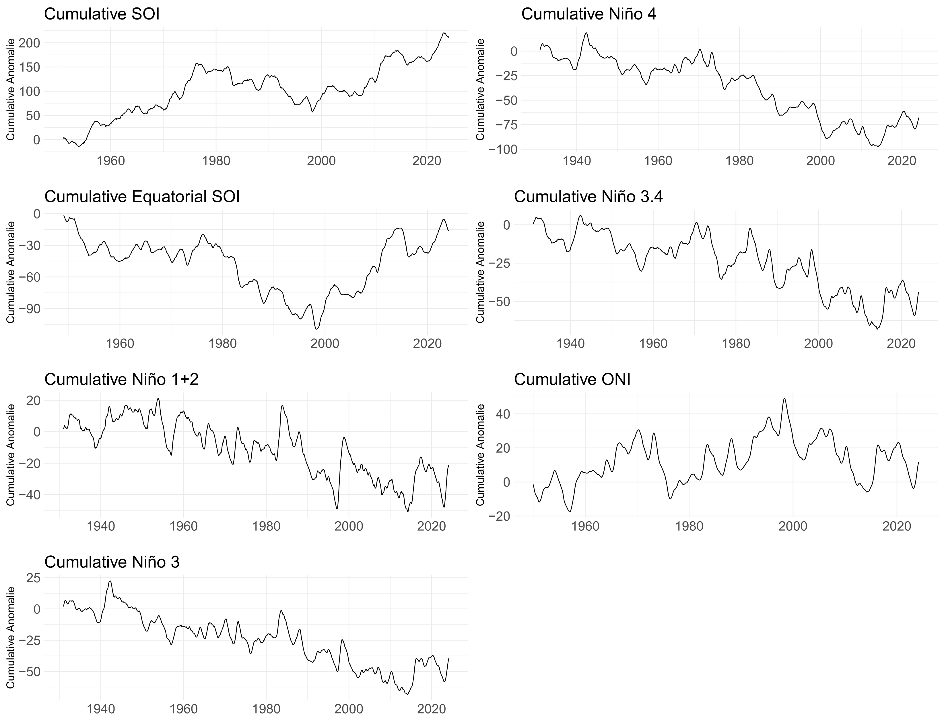
2.1.1. Datasets
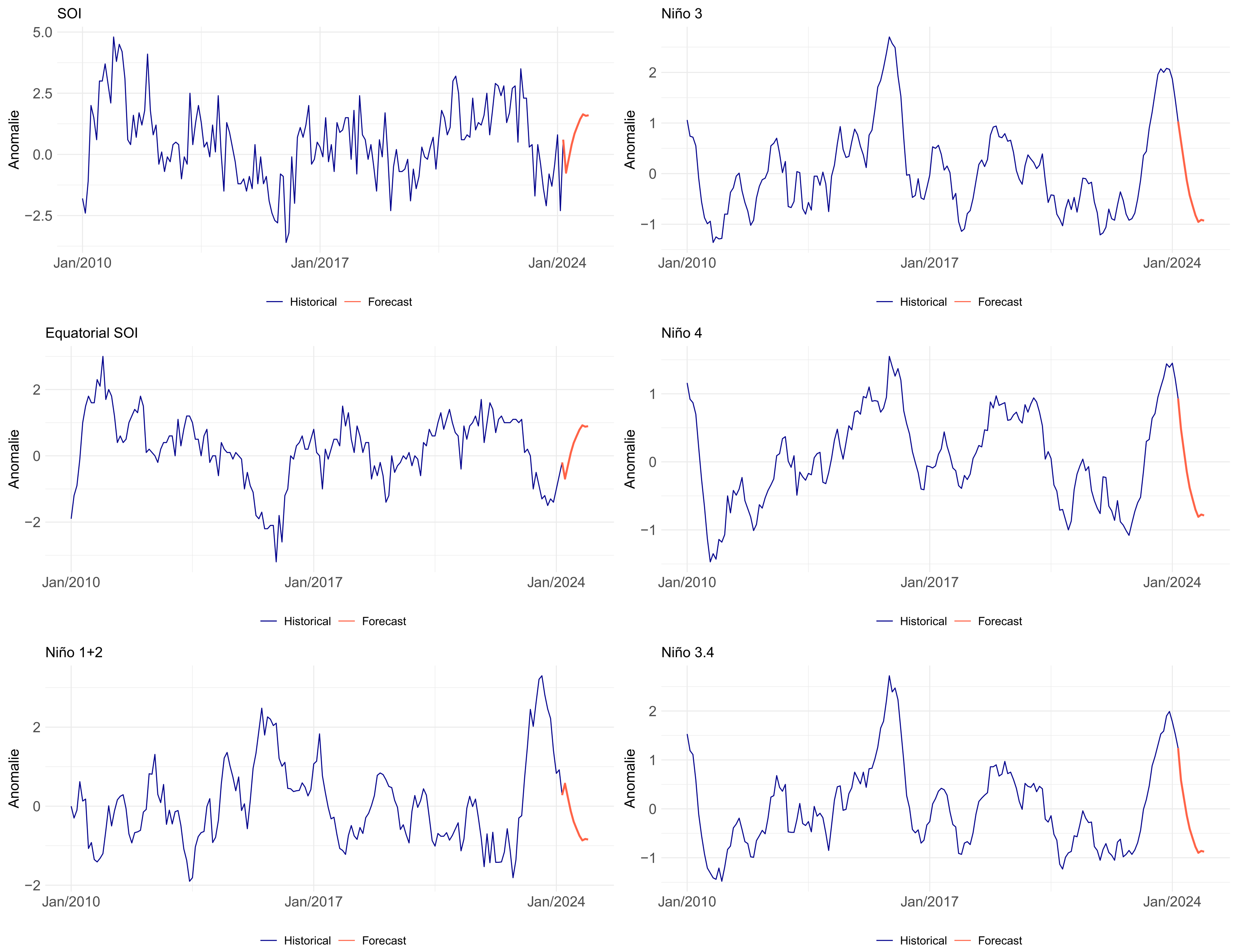
2.1.2. Extrapolation of Climate Variables
2.2. Modeling
2.2.1. Periodic Autoregressive Model (PAR)
2.2.2. Periodic Autoregressive Model with Exogenous Variables (PARX)
2.2.3. Covariance (PAR-Cov and PARX-Cov)
- 1.
- Calculation of the covariance matrix .
- 2.
- Spectral decomposition.
- 3.
- Multivariate normal distribution.
2.3. Post-Processing
2.3.1. Performance Metrics
2.3.2. Fitting and Forecasting Windows
- (i)
- Fit the wind speed series for the in-sample period;
- (ii)
- Simulate scenarios of the out-of-sample period (using the observed values of climatic variables from the in-sample period);
- (iii)
- Compare the forecast values, calculated as the average of the scenarios, with the observed value;
- (iv)
- Record the errors obtained in the validation set.
2.3.3. Stochastic Simulation of Wind Speed Scenarios
2.3.4. Forecast of Wind Speed
3. Results
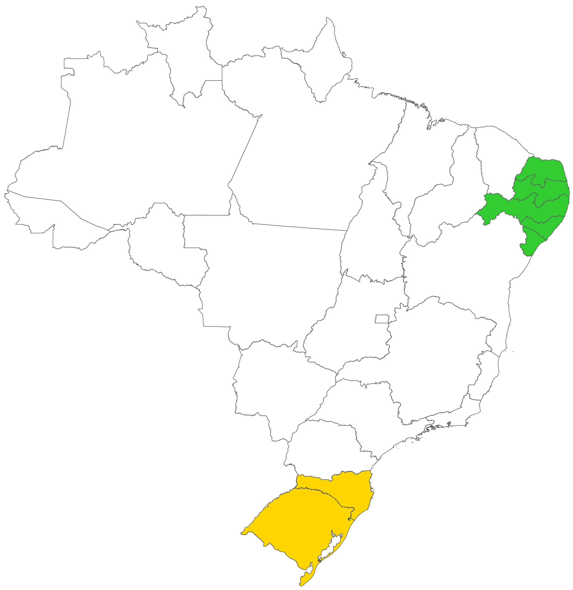
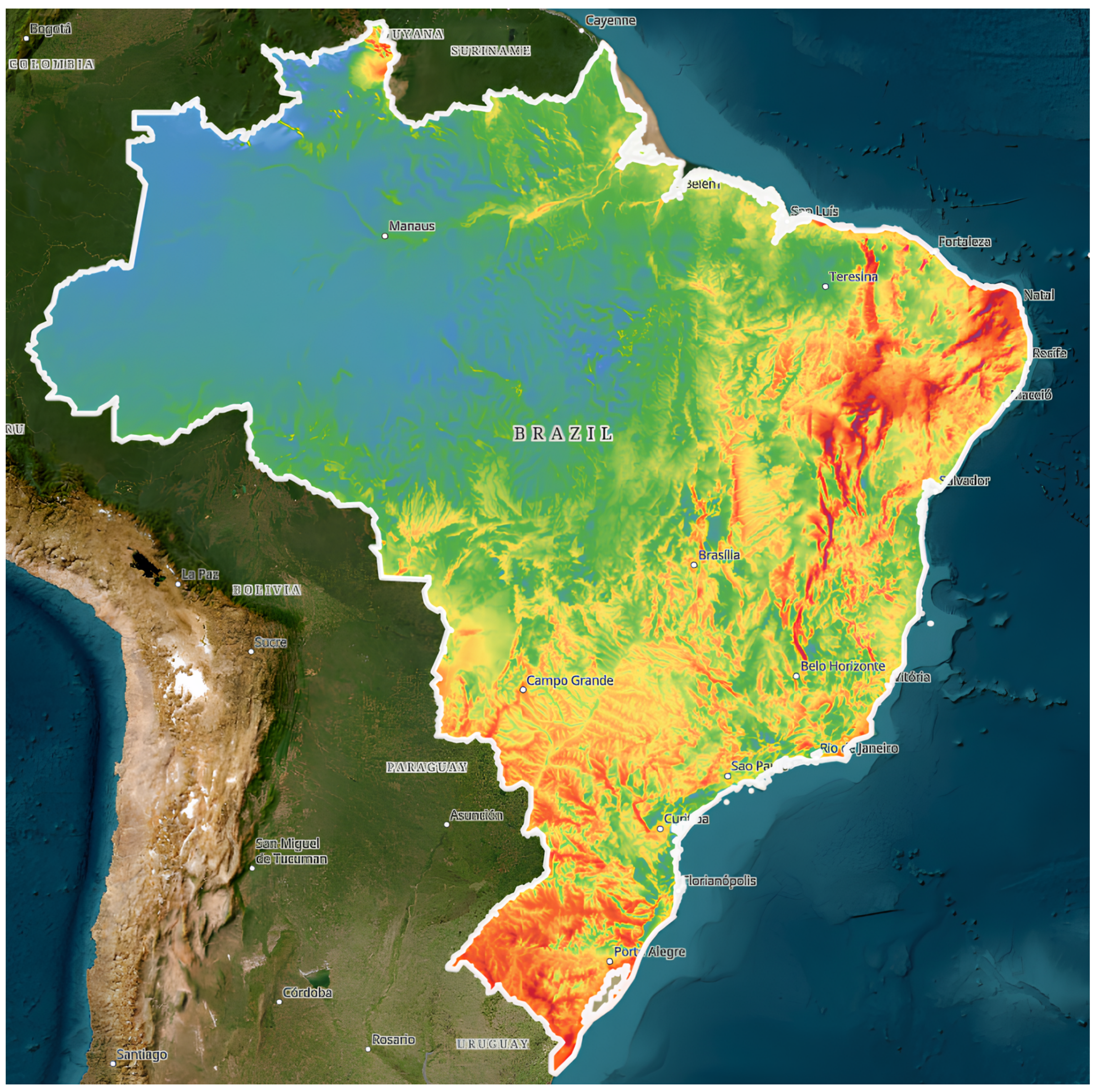
3.1. Descriptive Analysis of the Data
3.1.1. Wind Speed
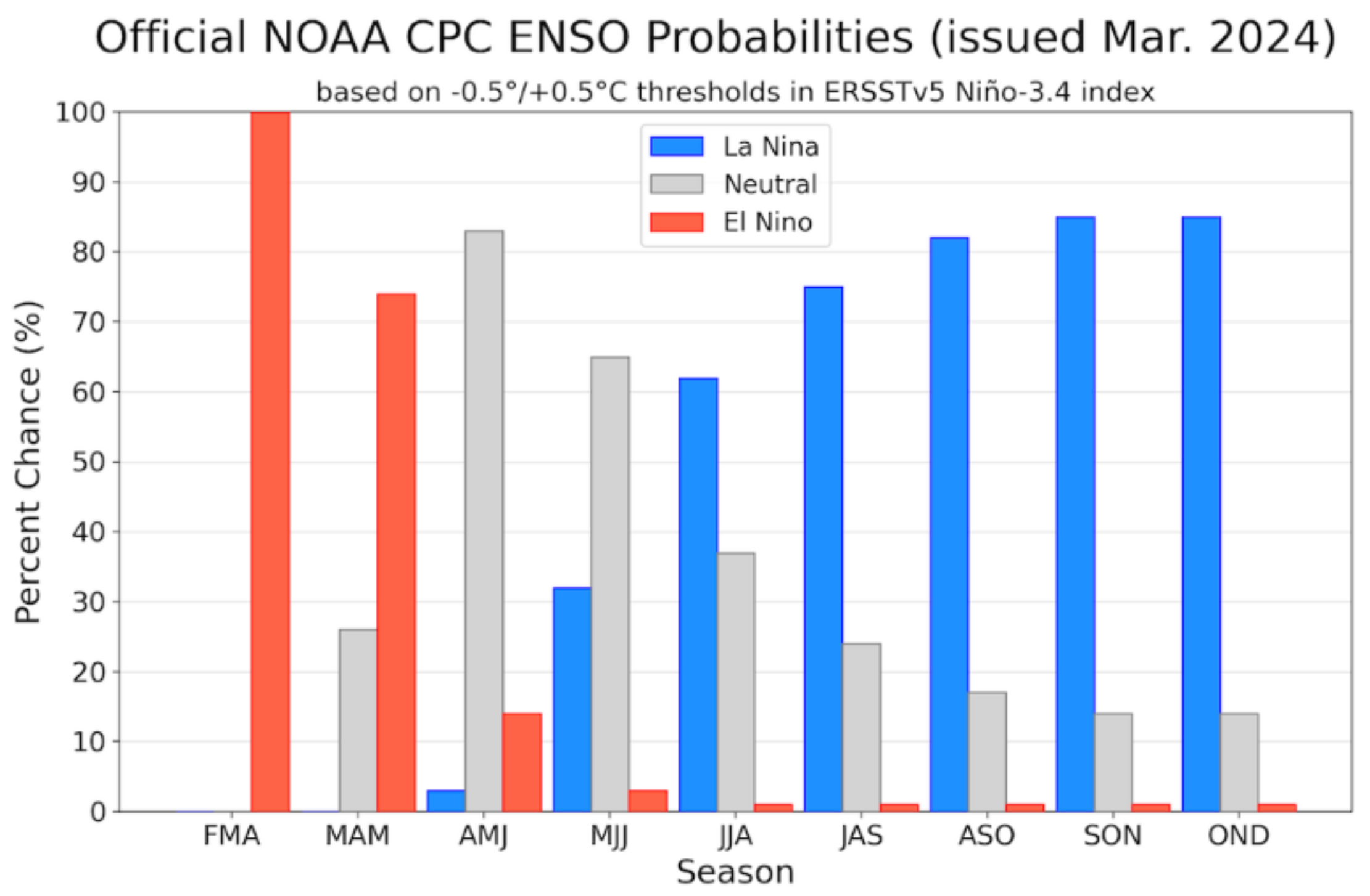
3.1.2. ENSO
3.1.3. Relationship Between Wind Speed and ENSO
3.2. Forecast of ENSO Indices
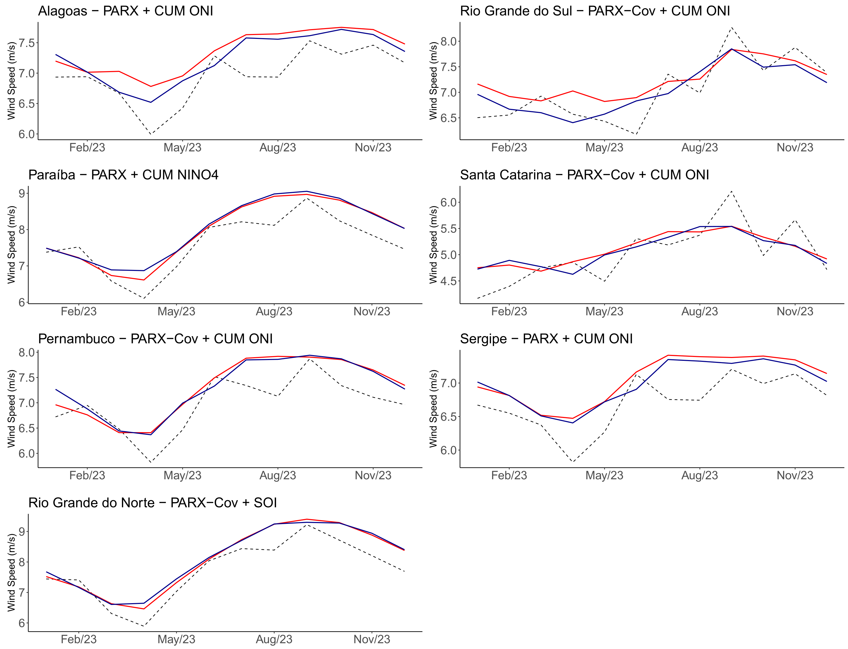
3.3. Wind Speed Simulation and Forecasting
4. Conclusions
Author Contributions
Funding
Data Availability Statement
Conflicts of Interest
References
- EPE. 2021. Available online: https://www.epe.gov.br/pt/publicacoes-dadosabertos/publicacoes/balanco-energetico-nacional-ben (accessed on 10 May 2023).
- Rigotti, J.A.; Carvalho, J.M.; Soares, L.M.; Barbosa, C.C.; Pereira, A.R.; Duarte, B.P.; Mannich, M.; Koide, S.; Bleninger, T.; Martins, J.R. Effects of hydrological drought periods on thermal stability of Brazilian reservoirs. Water 2023, 15, 2877. [Google Scholar] [CrossRef]
- Maceira, M.; Melo, A.; Pessanha, J.; Cruz, C.; Almeida, V.; Justino, T. Wind uncertainty modeling in long-term operation planning of hydro-dominated systems. In Proceedings of the 2022 17th International Conference on Probabilistic Methods Applied to Power Systems (PMAPS), Manchester, UK, 12–15 June 2022; pp. 1–6. [Google Scholar]
- Melo, G.; Barcellos, T.; Ribeiro, R.; Couto, R.; Gusmão, B.; Oliveira, F.L.C.; Maçaira, P.; Fanzeres, B.; Souza, R.C.; Bet, O. Renewable energy sources spatio-temporal scenarios simulation under influence of climatic phenomena. Electr. Power Syst. Res. 2024, 235, 110725. [Google Scholar] [CrossRef]
- Pinson, P. Wind energy: Forecasting challenges for its operational management. Stat. Sci. 2013, 28, 564–585. [Google Scholar] [CrossRef]
- Ferreira, P.G.C.; Oliveira, F.L.C.; Souza, R.C. The stochastic effects on the Brazilian Electrical Sector. Energy Econ. 2015, 49, 328–335. [Google Scholar] [CrossRef]
- Souza, R.C.; Marcato, A.; Dias, B.H.; Oliveira, F.L.C. Optimal operation of hydrothermal systems with hydrological scenario generation through bootstrap and periodic autoregressive models. Eur. J. Oper. Res. 2012, 222, 606–615. [Google Scholar] [CrossRef]
- EPE. Plano Nacional de Energia—PNE 2050. 2018. Available online: https://static.poder360.com.br/2020/12/PNE2050.pdf (accessed on 20 May 2022).
- do Nascimento Camelo, H.; Lucio, P.S.; Junior, J.B.V.L.; de Carvalho, P.C.M. A hybrid model based on time series models and neural network for forecasting wind speed in the Brazilian northeast region. Sustain. Energy Technol. Assess. 2018, 28, 65–72. [Google Scholar] [CrossRef]
- de Mattos Neto, P.S.; de Oliveira, J.F.; Júnior, D.S.d.O.S.; Siqueira, H.V.; Marinho, M.H.; Madeiro, F. An adaptive hybrid system using deep learning for wind speed forecasting. Inf. Sci. 2021, 581, 495–514. [Google Scholar] [CrossRef]
- Corrêa, C.S.; Schuch, D.A.; Queiroz, A.P.d.; Fisch, G.; Corrêa, F.d.N.; Coutinho, M.M. The long-range memory and the fractal dimension: A case study for Alcântara. J. Aerosp. Technol. Manag. 2017, 9, 461–468. [Google Scholar] [CrossRef]
- Lima, C.N.N.; Fernandes, C.A.C.; França, G.B.; de Matos, G.G. Estimation of the El Niño/La Niña impact in the intensity of Brazilian Northeastern winds. Anuário Inst. Geociênci. 2014, 37, 232–240. [Google Scholar] [CrossRef]
- Arpe, K.; Molavi-Arabshahi, M.; Leroy, S.A.G. Wind variability over the Caspian Sea, its impact on Caspian seawater level and link with ENSO. Int. J. Climatol. 2020, 40, 6039–6054. [Google Scholar] [CrossRef]
- Xu, Q.; Li, Y.; Cheng, Y.; Ye, X.; Zhang, Z. Impacts of climate oscillation on offshore wind resources in China seas. Remote Sens. 2022, 14, 1879. [Google Scholar] [CrossRef]
- Coria-Monter, E.; Salas de León, D.A.; Monreal-Gómez, M.A.; Durán-Campos, E. Satellite observations of the effect of the “Godzilla El Niño” on the Tehuantepec upwelling system in the Mexican Pacific. Helgol. Mar. Res. 2019, 73, 3. [Google Scholar] [CrossRef]
- Maçaira, P.; Thomé, A.; Cyrino Oliveira, F.; de Almeida, F. Time series analysis with explanatory variables: A systematic literature review. Environ. Model. Softw. 2018, 107, 199–209. [Google Scholar] [CrossRef]
- de Mendonça, M.J.C.; Pessanha, J.F.M.; de Almeida, V.A.; Medrano, L.A.T.; Hunt, J.D.; Junior, A.O.P.; Nogueira, E.C. Synthetic wind speed time series generation by dynamic factor model. Renew. Energy 2024, 228, 120591. [Google Scholar] [CrossRef]
- Ursu, E.; Pereau, J. Estimation and identification of periodic autoregressive models with one exogenous variable. J. Korean Stat. Soc. 2017, 46, 629–640. [Google Scholar] [CrossRef]
- Silveira, C.; Alexandre, A.; de Souza Filho, F.; Vasconcelos Junior, F.; Cabral, S. Monthly streamflow forecast for National Interconnected System (NIS) using Periodic Auto-regressive Endogenous Models (PAR) and Exogenous (PARX) with climate information. Braz. J. Water Resour. 2017, 22, e30. [Google Scholar] [CrossRef]
- Maçaira, P.M.; Oliveira, F.L.C.; Ferreira, P.G.C.; Almeida, F.V.N.d.; Souza, R.C. Introducing a causal PAR (p) model to evaluate the influence of climate variables in reservoir inflows: A Brazilian case. Pesqui. Oper. 2017, 37, 107–128. [Google Scholar] [CrossRef]
- Huang, X.; Maçaira, P.M.; Hassani, H.; Oliveira, F.L.C.; Dhesi, G. Hydrological natural inflow and climate variables: Time and frequency causality analysis. Phys. A Stat. Mech. Its Appl. 2019, 516, 480–495. [Google Scholar] [CrossRef]
- Duran, M.J.; Cros, D.; Riquelme, J. Short-term wind power forecast based on ARX models. J. Energy Eng. 2007, 133, 172–180. [Google Scholar] [CrossRef]
- Golia, S.; Grossi, L.; Pelagatti, M. Machine learning models and intra-daily market information for the prediction of Italian electricity prices. Forecasting 2022, 5, 81–101. [Google Scholar] [CrossRef]
- Iung, A.M.; Cyrino Oliveira, F.L.; Marcato, A.L.M. A review on modeling variable renewable energy: Complementarity and spatial—Temporal dependence. Energies 2023, 16, 1013. [Google Scholar] [CrossRef]
- Global Wind Atlas. Available online: https://globalwindatlas.info/en (accessed on 27 November 2023).
- de Aquino Ferreira, S.C.; Oliveira, F.L.C.; Maçaira, P.M. Validation of the representativeness of wind speed time series obtained from reanalysis data for Brazilian territory. Energy 2022, 258, 124746. [Google Scholar] [CrossRef]
- Gruber, K.; Klöckl, C.; Regner, P.; Baumgartner, J.; Schmidt, J. Assessing the Global Wind Atlas and local measurements for bias correction of wind power generation simulated from MERRA-2 in Brazil. Energy 2019, 189, 116212. [Google Scholar] [CrossRef]
- Olauson, J.; Bergkvist, M. Modelling the Swedish wind power production using MERRA reanalysis data. Renew. Energy 2015, 76, 717–725. [Google Scholar] [CrossRef]
- Renewables.ninja. Available online: https://www.renewables.ninja/ (accessed on 27 November 2023).
- Pfenninger, S.; Staffell, I. Long-term patterns of European PV output using 30 years of validated hourly reanalysis and satellite data. Energy 2016, 114, 1251–1265. [Google Scholar] [CrossRef]
- Staffell, I.; Pfenninger, S. Using bias-corrected reanalysis to simulate current and future wind power output. Energy 2016, 114, 1224–1239. [Google Scholar] [CrossRef]
- NOAA. Available online: https://www.ncei.noaa.gov/access/monitoring/enso/ (accessed on 31 March 2024).
- National Weather Service, Climate Prediction Center. Available online: https://www.cpc.ncep.noaa.gov/data/indices/ (accessed on 31 March 2024).
- International Research Institute. Available online: https://iri.columbia.edu/our-expertise/climate/enso/ (accessed on 31 March 2024).
- Barhmi, S.; Elfatni, O.; Belhaj, I. Forecasting of wind speed using multiple linear regression and artificial neural networks. Energy Syst. 2020, 11, 935–946. [Google Scholar] [CrossRef]
- James, G.; Witten, D.; Hastie, T.; Tibshirani, R.; Taylor, J. Linear regression. In An Introduction to Statistical Learning: With Applications in Python; Springer: Berlin/Heidelberg, Germany, 2023; pp. 69–134. [Google Scholar]
- Hipel, K.; McLeod, A. Time Series Modelling of Water Resources and Environmental Systems; Elsevier: Amsterdam, The Netherlands, 1994. [Google Scholar]
- McLeod, A. Diagnostic Checking Periodic Autoregression Models with Application. J. Time Ser. Anal. 1995, 15, 221–233. [Google Scholar] [CrossRef]
- Schwarz, G. Estimating the dimension of a model. Ann. Stat. 1978, 6, 461–464. [Google Scholar] [CrossRef]
- Vrieze, S. Model selection and psychological theory: A discussion of the differences between the Akaike information criterion (AIC) and the Bayesian information criterion (BIC). Psychol. Methods 2012, 17, 228–243. [Google Scholar] [CrossRef]
- Makubyane, K.; Maposa, D. Forecasting short-and long-term wind speed in Limpopo province using machine learning and Extreme Value Theory. Forecasting 2024, 6, 885–907. [Google Scholar] [CrossRef]
- Dismuke, C.; Lindrooth, R. Ordinary least squares. Methods Des. Outcomes Res. 2006, 93, 93–104. [Google Scholar]
- Suryawanshi, A.; Ghosh, D. Wind speed prediction using spatio-temporal covariance. Nat. Hazards 2015, 75, 1435–1449. [Google Scholar] [CrossRef]
- Ezzat, A.A.; Jun, M.; Ding, Y. Spatio-temporal short-term wind forecast: A calibrated regime-switching method. Ann. Appl. Stat. 2019, 13, 1484. [Google Scholar] [CrossRef]
- Jacondino, W.D.; da Silva Nascimento, A.L.; Calvetti, L.; Fisch, G.; Beneti, C.A.A.; da Paz, S.R. Hourly day-ahead wind power forecasting at two wind farms in northeast Brazil using WRF model. Energy 2021, 230, 120841. [Google Scholar] [CrossRef]
- de Souza, N.B.P.; Nascimento, E.G.S.; Santos, A.A.B.; Moreira, D.M. Wind mapping using the mesoscale WRF model in a tropical region of Brazil. Energy 2022, 240, 122491. [Google Scholar] [CrossRef]
- Mugware, F.W.; Sigauke, C.; Ravele, T. Evaluating wind speed forecasting models: A comparative study of CNN, DAN2, Random Forest and XGBOOST in diverse South African weather conditions. Forecasting 2024, 6, 672–699. [Google Scholar] [CrossRef]
- Charbeneau, R. Comparison of the two- and three-parameter log normal distributions used in streamflow synthesis. Water Resour. Res. 1978, 14, 149–150. [Google Scholar] [CrossRef]
- Pereira, M.; Oliveira, G.; Costa, C.; Kelman, J. Stochastic streamflow models for hydroeletric systems. Water Resour. Res. 1984, 20, 379–390. [Google Scholar] [CrossRef]
- R Core Team. R: A Language and Environment for Statistical Computing; R Foundation for Statistical Computing: Vienna, Austria, 2022. [Google Scholar]
- Paparoditis, E.; Politis, D.N. The asymptotic size and power of the augmented Dickey–Fuller test for a unit root. Econom. Rev. 2018, 37, 955–973. [Google Scholar] [CrossRef]
- Escobari, D.; Garcia, S.; Mellado, C. Identifying bubbles in Latin American equity markets: Phillips-Perron-based tests and linkages. Emerg. Mark. Rev. 2017, 33, 90–101. [Google Scholar] [CrossRef]
- Barnston, A. Why Are There So Many ENSO Indexes, Instead of Just One? Available online: https://www.climate.gov/news-features/blogs/enso/why-are-there-so-many-enso-indexes-instead-just-one (accessed on 27 November 2023).
- Bjerknes, J. Atmospheric teleconnections from the equatorial Pacific. J. Phys. Oceanogr. 1969, 97, 163–172. [Google Scholar]
- Barnston, A.; Chelliah, M.; Goldenberg, S. Documentation of a highly ENSO-related SST region in the equatorial Pacific. Atmosphere-Ocean 1997, 35, 367–383. [Google Scholar]
- IRENA. 2021. Available online: https://www.irena.org/newsroom/pressreleases/2021/Apr/World-Adds-Record-New-Renewable-Energy-Capacity-in-2020 (accessed on 10 May 2023).


| Windows | In-Sample | Out-of-Sample |
|---|---|---|
| 1 | Jan/1980–Dec/2013 | Jan/2014–Dec/2018 |
| 2 | Jan/1980–Dec/2014 | Jan/2015–Dec/2019 |
| 3 | Jan/1980–Dec/2015 | Jan/2016–Dec/2020 |
| 4 | Jan/1980–Dec/2016 | Jan/2017–Dec/2021 |
| 5 | Jan/1980–Dec/2017 | Jan/2018–Dec/2022 |
| 6 | Jan/1980–Dec/2022 | Jan/2023–Dec/2023 |
| 7 | Jan/1980–Dec/2023 | Jan/2024–Dec/2024 |
| State | Mean | Median | Standard Deviation | Coefficient of Variation | Skewness | Kurtosis |
|---|---|---|---|---|---|---|
| Alagoas | 7.30 | 7.36 | 0.53 | 0.07 | −0.40 | 2.87 |
| Paraíba | 7.97 | 8.12 | 0.93 | 0.12 | −0.53 | 2.94 |
| Pernambuco | 7.31 | 7.43 | 0.69 | 0.09 | −0.45 | 2.90 |
| Rio Grande do Norte | 8.15 | 8.34 | 1.13 | 0.14 | −0.55 | 2.87 |
| Rio Grande do Sul | 7.23 | 7.21 | 0.64 | 0.09 | 0.24 | 3.36 |
| Santa Catarina | 5.08 | 5.06 | 0.44 | 0.09 | 0.13 | 2.71 |
| Sergipe | 7.05 | 7.12 | 0.48 | 0.07 | −0.21 | 2.94 |
| State | SOI | Equatorial SOI | Niño 1+2 | Niño 3 | Niño 4 | Niño 3.4 | ONI |
|---|---|---|---|---|---|---|---|
| Alagoas | 0.426 | 0.93 | 0.123 | 0.801 | 0.662 | 0.801 | 0.645 |
| Yes | Yes | Yes | Yes | Yes | Yes | Yes | |
| Paraíba | 0.262 | 0.918 | 0.013 | 0.312 | 0.097 | 0.197 | 0.788 |
| Yes | Yes | No | Yes | No | Yes | Yes | |
| Pernambuco | 0.587 | 0.73 | 0.02 | 0.168 | 0.117 | 0.204 | 0.682 |
| Yes | Yes | No | Yes | Yes | Yes | Yes | |
| Rio Grande do Norte | 0.065 | 0.852 | 0.023 | 0.787 | 0.193 | 0.26 | 0.609 |
| No | Yes | No | Yes | Yes | Yes | Yes | |
| Rio Grande do Sul | 0.492 | 0.102 | 0.308 | 0.075 | 0.749 | 0.335 | 0.093 |
| Yes | Yes | Yes | No | Yes | Yes | No | |
| Santa Catarina | 0.167 | 0.174 | 0.001 | 0.545 | 0.395 | 0.378 | 0.259 |
| Yes | Yes | No | Yes | Yes | Yes | Yes | |
| Sergipe | 0.466 | 0.89 | 0.099 | 0.494 | 0.354 | 0.925 | 0.755 |
| Yes | Yes | No | Yes | Yes | Yes | Yes |
| Index | Coefficients | Estimated Value | Standard Deviation | p-Value | |
|---|---|---|---|---|---|
| SOI | (Intercept) | 0.275 | 0.036 | ≈0 | 0.528 |
| ONI | −1.349 | 0.043 | ≈0 | ||
| Equatorial SOI | (Intercept) | 0.001 | 0.017 | 0.938 | 0.701 |
| ONI | −0.909 | 0.020 | ≈0 | ||
| Niño 1+2 | (Intercept) | −0.046 | 0.026 | 0.072 | 0.444 |
| ONI | 0.811 | 0.030 | ≈0 | ||
| Niño 3 | (Intercept) | −0.046 | 0.011 | ≈0 | 0.831 |
| ONI | 0.898 | 0.014 | ≈0 | ||
| Niño 4 | (Intercept) | −0.072 | 0.010 | ≈0 | 0.792 |
| ONI | 0.728 | 0.013 | ≈0 | ||
| Niño 3.4 | (Intercept) | −0.052 | 0.009 | ≈0 | 0.882 |
| ONI | 0.837 | 0.010 | ≈0 |
| State | Metric | PAR | Best Model | Best Model | Improvement (%) |
|---|---|---|---|---|---|
| Alagoas | RMSE | 0.4057 | PARX + CUM ONI | 0.401 | 1.15 |
| MAE | 0.312 | PARX + CUM ONI | 0.3077 | 1.36 | |
| 0.476 | PARX + CUM ONI | 0.4878 | 2.48 | ||
| Paraíba | RMSE | 0.5013 | PARX + CUM NINO4 | 0.4908 | 2.09 |
| MAE | 0.3867 | PARX + CUM ONI | 0.3782 | 2.19 | |
| 0.7418 | PARX + CUM NINO4 | 0.7522 | 1.4 | ||
| Pernambuco | RMSE | 0.4714 | PARX + CUM ONI | 0.4673 | 0.87 |
| MAE | 0.3688 | PARX-Cov + CUM ONI | 0.3632 | 1.49 | |
| 0.6 | PARX-Cov + CUM NINO3.4 | 0.6068 | 1.12 | ||
| Rio Grande do Norte | RMSE | 0.52 | PARX-Cov + SOI | 0.5102 | 1.88 |
| MAE | 0.4064 | PARX + CUM ONI | 0.3996 | 1.69 | |
| 0.8045 | PARX-Cov + SOI | 0.8102 | 0.71 | ||
| Rio Grande do Sul | RMSE | 0.4888 | PARX-Cov + CUM ONI | 0.4748 | 2.87 |
| MAE | 0.3867 | PARX + CUM ONI | 0.3798 | 1.8 | |
| 0.2263 | PARX-Cov + CUM ONI | 0.27 | 19.29 | ||
| Santa Catarina | RMSE | 0.3055 | PARX-Cov + CUM ONI | 0.2974 | 2.65 |
| MAE | 0.2479 | PARX-Cov + CUM ONI | 0.2368 | 4.47 | |
| 0.429 | PARX-Cov + CUM ONI | 0.459 | 6.99 | ||
| Sergipe | RMSE | 0.3829 | PARX + CUM ONI | 0.3795 | 0.89 |
| MAE | 0.2931 | PARX + CUM ONI | 0.2887 | 1.53 | |
| 0.422 | PARX + CUM ONI | 0.4321 | 2.4 |
| Model | Frequency (Out of 21) |
|---|---|
| PARX + CUM ONI | 10 |
| PARX-Cov + CUM ONI | 6 |
| PARX + CUM NINO4 | 2 |
| PARX-Cov + SOI | 2 |
| PARX-Cov + CUM NINO3.4 | 1 |
| State | Best Model |
|---|---|
| Alagoas | PARX + CUM ONI |
| Paraíba | PARX + CUM NINO4 |
| Pernambuco | PARX-Cov + CUM ONI |
| Rio Grande do Norte | PARX-Cov + SOI |
| Rio Grande do Sul | PARX-Cov + CUM ONI |
| Santa Catarina | PARX-Cov + CUM ONI |
| Sergipe | PARX + CUM ONI |
Disclaimer/Publisher’s Note: The statements, opinions and data contained in all publications are solely those of the individual author(s) and contributor(s) and not of MDPI and/or the editor(s). MDPI and/or the editor(s) disclaim responsibility for any injury to people or property resulting from any ideas, methods, instructions or products referred to in the content. |
© 2025 by the authors. Licensee MDPI, Basel, Switzerland. This article is an open access article distributed under the terms and conditions of the Creative Commons Attribution (CC BY) license (https://creativecommons.org/licenses/by/4.0/).
Share and Cite
Couto, R.A.; Maçaira Louro, P.M.; Cyrino Oliveira, F.L. Forecasting Wind Speed Using Climate Variables. Forecasting 2025, 7, 13. https://doi.org/10.3390/forecast7010013
Couto RA, Maçaira Louro PM, Cyrino Oliveira FL. Forecasting Wind Speed Using Climate Variables. Forecasting. 2025; 7(1):13. https://doi.org/10.3390/forecast7010013
Chicago/Turabian StyleCouto, Rafael Araujo, Paula Medina Maçaira Louro, and Fernando Luiz Cyrino Oliveira. 2025. "Forecasting Wind Speed Using Climate Variables" Forecasting 7, no. 1: 13. https://doi.org/10.3390/forecast7010013
APA StyleCouto, R. A., Maçaira Louro, P. M., & Cyrino Oliveira, F. L. (2025). Forecasting Wind Speed Using Climate Variables. Forecasting, 7(1), 13. https://doi.org/10.3390/forecast7010013