Dynamic Bayesian Network Model for Overhead Power Lines Affected by Hurricanes

Abstract

This paper investigates the dynamics of Hurricane-Induced Failure (HIF) by developing a probabilistic framework using a Dynamic Bayesian Network (DBN) model. The model captures the complex interplay of factors influencing Hurricane Wind Speed Intensity (HWSI) and its impact on asset failures. In the proposed DBN model, the pole failure mechanism is represented using Bayesian probabilistic principles, encompassing bending elasticity endurance and the foundational strength of the system poles. To characterize the stochastic properties of HIF, Monte Carlo simulation (MCS) is employed in conjunction with fragility curves (FC) and the scenario reduction (SCENRED) algorithm. The proposed DBN model evaluates the probability of asset failure and compares the results using stochastic Monte Carlo simulation based on the fragility curve scenario reduction algorithm (FC-MCS-SCENRED) model. The results are validated on a standard IEEE 15 bus and IEEE 33 bus radial distribution system as a case study. The DBN results show that they are consistent with the data obtained using the FC-MCS-SCENRED model. The results also reveal that the HWSI plays a critical role in determining HIF rates and the likelihood of asset failures. These findings hold significant implications for the inspection and maintenance scheduling of distribution overhead power lines susceptible to hurricane-induced impacts.

1. Introduction

1.1. Motivation

Severe weather events, such as hurricanes and floods, have become more frequent in recent years [1]. The majority of power outages occur in power distribution systems (PDSs) due to these extreme weather conditions [2], while earthquakes can cause damage to substations [3] and, in certain situations, the transmission system and generators [4,5]. Compared to the power transmission system, the PDSs that deliver electricity to individual customers from neighboring substations are more susceptible to damage and are more likely to cause power outages for customers during extreme weather [5].

Among these natural disasters, hurricanes stand out as one of the most destructive [6], inflicting extensive harm to infrastructure, residences, and communities [7,8,9]. Hurricanes have the potential to exert a profound and enduring influence on PDSs, which in turn can have far-reaching implications for public safety, economic productivity, and overall quality of life [10,11,12,13,14]. Given the critical role that PDSs play in society, it becomes imperative to gain a comprehensive understanding of the impact hurricanes have on these systems and to formulate effective strategies for enhancing their resilience [15,16].

Overhead PDSs, which include conductors and wood utility poles, are especially vulnerable to hurricanes [17], with high winds, storm surges, and heavy rainfall resulting in extended outages and disrupting the power supply [18]. For instance, Hurricane Hugo in 1989 resulted in more than 15,000 pole failures, while Hurricane Wilma and Hurricane Katrina in 2005 caused damage to over 12,000 poles [19]. This heightened vulnerability primarily stems from the rapid decay of wood material and the substantial exposure to wind forces. In response to this issue, significant attention has been directed towards risk assessment and life cycle cost analysis over the past decade. These approaches aim to evaluate system vulnerabilities and formulate cost-effective management strategies. To execute such risk assessments, it is necessary to estimate the probability of failure for individual vulnerable components, such as wood utility poles.

1.2. Literature Review

Several research articles have been published in the past, with a particular emphasis on enhancing the resilience of overhead PDSs during hurricanes, including predictive modeling, proactive measures, risk assessment, and vulnerability analysis.

It is usually assumed that the system is exposed to the uniform weather conditions by modeling weather as a static event, simplifying the modeling process by not accounting for regional weather variations [20]. However, in practice, power system (PS) grid lines encounter various Hurricane Wind Speed Intensity (HWSI) conditions across different times and environments [21,22]. PS networks typically consist of numerous dynamic components that evolve over time. This inherent dynamism poses a challenge for current methods to accurately assess the evolving state of network resilience [23]. For instance, the wood of utility poles, being a natural material, undergoes degradation under the effect of hurricanes. Consequently, the performance of PDSs can exhibit substantial variations throughout their operational lifecycles [24].

To help assess the vulnerability of utility poles against wind stress, the focus is paid on developing multi-dimensional wind fragility functions specifically for utility poles in [25]. These functions are essential for enhancing resilience against hurricane-induced effects on utility poles. The component fragility models, including that of utility poles, have been used in [26] to develop a PS performance model for rapid assessments of various network topologies of the distribution network. A probabilistic modeling approach for quantifying the hurricane resilience PDSs is discussed in [27]. In this study, the focus is paid on to the response of the most critical and vulnerable components like distribution nodes and lines (which include distribution poles and conductors between poles) via the use of component fragility models.

To predict and mitigate power line outages during hurricanes, a Bayesian network (BN) line outage prediction model is used in [21] to enhance the resilience of PDSs against hurricane events. In [24], to capture the failure probability (FP) of the PDS utility poles, fragility surfaces for the poles are obtained using modeling based on physics, and finally, the failure rate is determined through the BN analysis. The physics-based models excel at forecasting failures during high-wind conditions, but their efficacy reduces when applied to lower wind speeds [28]. On the other hand, BNs are renowned for their ability to handle causal relationships among various variables, but it is important to note that BNs are typically applied to static systems. However, for PSs to remain static or at equilibrium, this is often not the case because the majority of the system’s performance fluctuates with the passage of time or is dynamic in nature. Thus, the temporal element needs to be tackled [29]. In addition to this, there are also data-driven models that have been effective in forecasting typical scenarios but struggle with extreme events, where data might be limited [28].

Over the past 20 years, large datasets have been used by statistical learning and machine learning techniques to develop outage prediction models [30]. Figure 1a shows different modern learning approaches being exploited in the field of power outage predictions. Some of the most widely used machine learning algorithms used in the context of power outage predictions are shown is Figure 1b.

A number of Random Forest-based power outage prediction models were created in [32] in order to precisely forecast future storms with short run times. Damage modeling of towers and poles is essential in the context of power outage predictions. According to a case study on tower modeling in [33] that used the gradient boosting technique, the technique works best when model accuracy is prioritized over model efficiency. According to [34], the ensemble learning technique AdaBoost worked well for estimating weather-related power outages at the distribution side. In [35], where distinct spatiotemporal models based on long short-term memory (LSTM) and convolutional neural networks (CNN) were constructed utilizing weather and outage data, deep learning has proven to be a useful tool for customer outage forecasting. In terms of performance, a power outage prediction model based on deep belief networks (DBNs) that was employed in [36] also shows promise. A classification decision tree is utilized in [37] to assess storm severity to improve power outage prediction by including storm severity classification into an outage prediction model (OPM).

1.3. Paper Contribution

This article’s primary contribution is to enhance the effectiveness of risk assessment for probabilistic system line ($\mathrm{S}\mathrm{L}$) failure predictions with the help of a Dynamic Bayesian Network (DBN). The research centers on the concept that power $\mathrm{S}\mathrm{L}$ outages at a specific location could be influenced by other points of failure during hurricane events. This suggests that power interruptions may be impacted by the dynamic nature of hurricane events across the grid. By employing the DBN approach, the study aims to estimate the dynamic changes in the probability of asset failure over time. The results obtained using this proposed method are then compared with those derived from the FC-MCS-SCENRED model. The outcomes of this study offer valuable insights into understanding the influence of time-dependent HIF and predicting the likelihood of ${\mathrm{S}}_{\mathrm{L}}$ failures.

1.4. Paper Organization

The paper is organized as follows. Section 2 formulates the overhead line failure analysis in PDSs. Section 3 presents the applications of DBN to the IEEE 15 bus system as a case study. The results and discussion are presented in Section 4. Finally, the conclusion is presented in the last section.

2. Overhead Line Failure Model

The objective of the overhead line failure model is to evaluate the probability of the failure of a system line. This line failure could be due to extreme winds or trees falling. In the wind scenario, wire breakage and pole bending failure are common failure modes, whereas in the tree-fall scenario, wire breakage and short circuit are common failure modes. In the present study, we are only concerned with the wind scenario.

When the maximal stress from external loads surpasses the poles’ fiber strength in a wind situation, pole failure takes place. When the maximum stress brought on by external loads surpasses the breaking strength of wires, wire breakage occurs. In the proposed model, it is assumed that a system line fails either due to the failure of poles or conductors. For a given failure mode, the associated failure probability is given by Equation (1) [38]:

$$\mathrm{F}\mathrm{P}=\mathrm{P}\left[\mathrm{G}\left({\mathrm{x}}_{\mathrm{i}}\right)\le 0\right]$$

(1)

where $\mathrm{G}\left({\mathrm{x}}_{\mathrm{i}}\right)$ is a metric called the limit state function and quantifies survival or failure, and ${\mathrm{x}}_{\mathrm{i}}$ is a set of random variables involved. In the context of the structural reliability of the component (pole/wire), the limit state function, $\mathrm{G},$ in its most fundamental form is given by Equation (2) [38]:

$$\mathrm{F}\mathrm{P}=\mathrm{P}[\mathrm{R}-\mathrm{S}\le 0]$$

(2)

where $\mathrm{R}$ represents resistance of the component (pole/wire) and $\mathrm{S}$ represents load/stress applied. Poles and wires are subjected to wind load in the wind scenario. The National Electrical Safety Code (NESC) (IEEE 2017) states that Equation (3) mentioned below can be used to determine the wind pressure, S, on poles and wires.

$$\mathrm{S}=0.5 {\mathsf{\rho }}_{\mathrm{a}}{\mathrm{k}}_{\mathrm{z}}\mathrm{G}{\mathrm{C}}_{\mathrm{f}}{\mathrm{U}}_{\mathrm{p}}^2$$

(3)

where G is the gust response factor; ${\mathrm{C}}_{\mathrm{f}}$ is the force coefficient; ${\mathsf{\rho }}_{\mathrm{a}}$ is the air density; ${\mathrm{k}}_{\mathrm{z}}$ is the velocity pressure exposure coefficient; and ${\mathrm{U}}_{\mathrm{p}}$ = projected 3 s gust wind speed. In the projected 3 s gust wind speed, ${\mathrm{U}}_{\mathrm{p}}$ is the 3 s gust wind speed and U for poles. The estimated 3 s gust wind speed up for wires is equal to Usin(α), where α is the wind attack angle, as wires are only exposed to the wind component perpendicularly. The probability of failure for the component (pole/wire) can be derived as follows [19]:

$$\mathrm{F}\mathrm{P}={\int }_{\mathrm{t}}^{.}\mathrm{P}\left[\mathrm{G}\right({\mathrm{x}}_{\mathrm{i}})<0]{\mathrm{f}}_{\mathsf{\sigma }}\left(\mathrm{t}\right)\mathrm{d}\mathrm{t}$$

(4)

where $\mathsf{\sigma }$ defines wind speed, ${\mathrm{f}}_{\mathsf{\sigma }}\left(\mathrm{t}\right)$ is the probability density function (PDF) of wind speed, and $\mathrm{P}\left[\mathrm{G}\right({\mathrm{x}}_{\mathrm{i}})<0]$ is the fragility function, which defines the conditional probability of failure. Hurricane events are described by the Poisson process of constant rate. In a Poisson process, it is the exponential distribution, which is commonly used to model the time between events, for example, the time between consecutive pole failures [27]. This usually constant rate is the failure rate, a specific number derived from statistical data and can be used to express the failure characteristics [39]. Therefore, if ${\mathsf{\lambda }}_{\mathrm{h}}$ denotes the failure rate of $\mathrm{i}$th component (pole/wire) such that

$${\mathsf{\lambda }}_{\mathrm{h}}={\mathrm{A}}_{\mathrm{i}}\times {\mathrm{e}}^{\left({\mathrm{B}}_{\mathrm{i}}\times \mathsf{\sigma }\right)}$$

(5)

where ${\mathrm{A}}_{\mathrm{i}}$ and ${\mathrm{B}}_{\mathrm{i}}$ represent the component (pole/wire) coefficients [40], then the probability function is given by Equation (6) [27]:

$${\mathrm{f}}_{\mathsf{\sigma }}(\mathrm{t})=\left\{\begin{array}{c}{\mathsf{\lambda }}_{\mathrm{h}}{\mathrm{e}}^{-{\mathsf{\lambda }}_{\mathrm{h}}\mathrm{t}}, \mathrm{t}\ge 0\\ \hspace{1em}\hspace{1em}0, \mathrm{t}<0\end{array}\right.$$

(6)

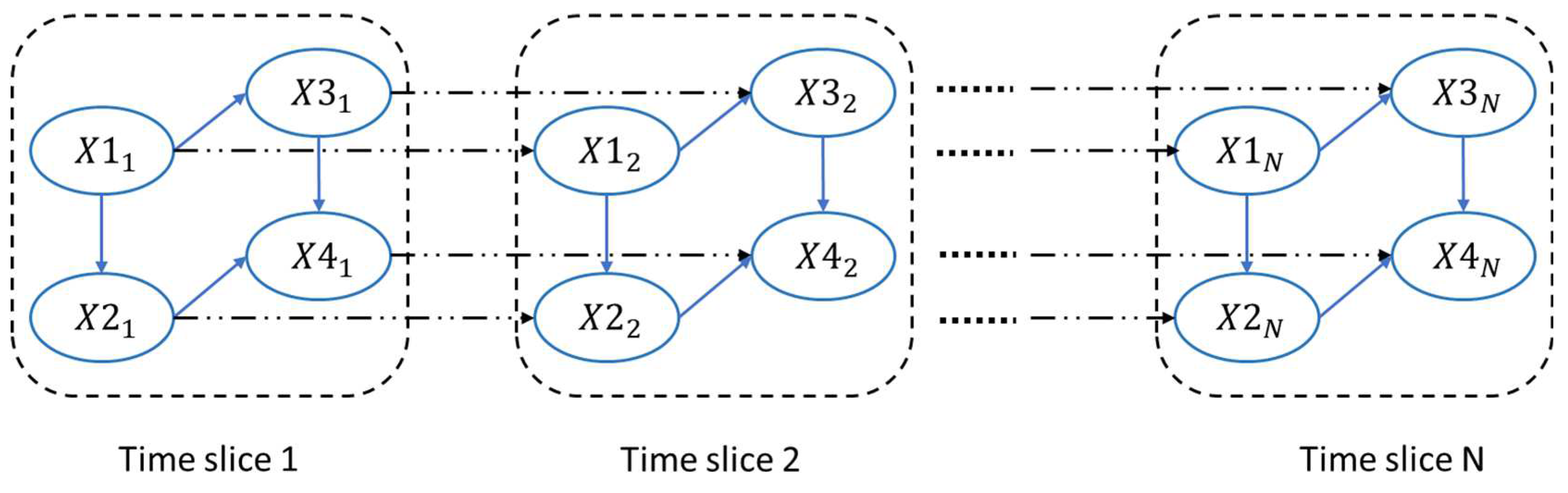
2.1. Dynamic Bayesian Network (DBN)

A BN serves as a probabilistic approach employed for accidental modeling in multiple fields of study [41,42,43,44]. A BN risk model aids in the identification of crucial factors responsible for causing accidents. This includes both direct and indirect factors [45,46]. This probabilistic method visually depicts the causal connections between variables and provides a comprehensive qualitative and quantitative description of their complex interrelationships [47,48,49]. For instance, to account for the overhead line failure, if system line failure is considered event A and HWSI hitting the system line is considered event B, then the event’s probability for the next system line in a BN is given by Equation (7).

$$\mathrm{P}\left(\mathrm{A}|\mathrm{B}\right)={\displaystyle \frac{\mathrm{P}\left(\mathrm{B}|\mathrm{A}\right).\mathrm{P}\left(\mathrm{A}\right)}{\mathrm{P}\left(\mathrm{B}\right)}}$$

(7)

where,

$\mathrm{P}\left(\mathrm{A}\right)$: the prior probability of event A.

$\mathrm{P}\left(\mathrm{B}\right)$: the prior probability of event B.

$\mathrm{P}\left(\mathrm{A}|\mathrm{B}\right)$: the conditional probability of event A provided event B has already taken place.

$\mathrm{P}\left(\mathrm{B}|\mathrm{A}\right)$: the conditional probability of event B provided event A has already taken place.

The prior probabilities of the event, which indicate the marginal probabilities [50], also represent the component state at the first time instant, i.e., t = 0. These are the probabilities under the failure states (expressed as 1) or normal states (expressed as 0). If the component has just started working, it can be considered that the failure probability is 0 [39]; that is, if ${\mathrm{X}}_0^{\mathrm{i}}$ denotes the $\mathrm{i}$th node of a variable at $\mathrm{t}=0$, then

$$\mathrm{P}{(\mathrm{X}}_0^{\mathrm{i}}=0)=1$$

(8a)

$$\mathrm{P}{(\mathrm{X}}_0^{\mathrm{i}}=1)=0$$

(8b)

In the present work, to monitor the degradation of overhead power distribution lines in real time, a “static” BN model is transformed into a “dynamic” model known as a DBN. The addition of a time dimension to the classical BN results in a DBN. The DBN facilitates the interaction between nodes/variables at distinct time steps and can be used for tracking the performance of system’s evolution provided the evidence recorded at an earlier time slice/step. This helps in estimating the system’s resilience state, provided its initial state is given. The key characteristic of a DBN, which is a directed acyclic graphical model, is that the elements are linked through different time steps [29]. A DBN reveals the conditional independence relationships among a group of random variables at different slices of time, denoted as t = (1, 2, 3..., N) [51,52]. A static BN model encompassing four random variables is shown in Figure 2, and ‘N’, the number of time slices of a DBN model, is shown in Figure 3. The overhead power lines can be affected by several variables related to hurricanes, like HWSI, wind duration, wind direction, rainfall, etc.

This study targets a comparison of the outcomes of the DBN model with a stochastic approach called the FC-MCS-based-SCENRED model for a standard IEEE 15 bus system and IEEE 33 bus system affected by HWSI. The stochastic approach calculates the FP of the distribution poles for the standard system affected by HWSI over time. A degraded power line typically fails because of the stress of HWSI, which is mainly considered as a random variable in the present study. HWSI data are used as input data. In this study, the vegetation effects are not considered. The failure mode of utility poles considered only the bending mode, which is the most prevalent type of failure mode observed in distribution poles [24]. Therefore, the scope of the present study is restricted to the bending elasticity endurance and the foundational strength of the poles, which resist the HWSI-induced stress.

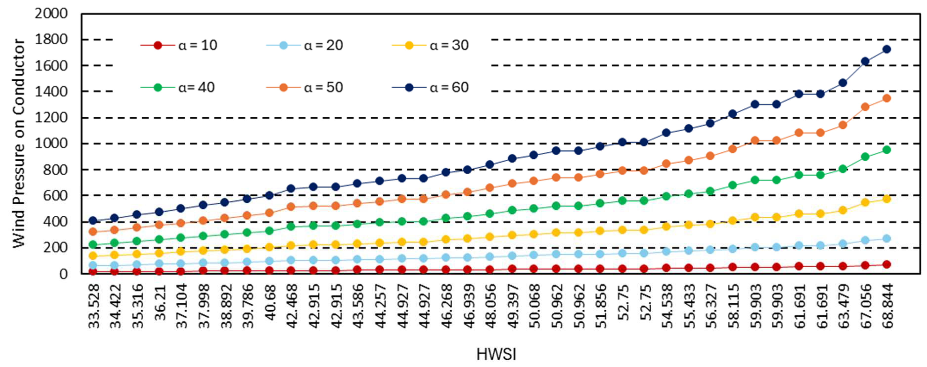
2.2. Uncertainty Modeling

2.2.1. Scenario-Based Approach

To capture the uncertainties linked with the overhead line damage caused by the uncertain hurricane event, a scenario-based method was used in this study. A scenario-based simulation method was adopted to mimic real-world conditions and to compensate for the lack of real historical data. In this method, we began by utilizing HWSI data to establish a probability distribution function (PDF). Subsequently, we generated a finite set of scenarios (1000 random scenarios as the stopping criteria) for overhead line via the Monte Carlo simulation (MCS) algorithm based on this PDF [53,54]. This choice was grounded in prior research articles [21,55,56], which have demonstrated that utilizing 1000 scenarios ensures the accuracy of ${\mathrm{S}}_{\mathrm{L}}$ outage predictions. However, analyzing such a huge number of scenarios can be challenging and computationally intensive, particularly when conducting pre-disaster system optimization. To address these challenges, we applied the scenario reduction (SCENRED) algorithm to the FC-MCS model of the system components [21]. Initially, we generated 1000 PDS through the system component’s FC-MCS, as detailed in step 4 for model validation. Subsequently, we employed the SCENRED algorithm, implemented in MATLAB 2023a using the K-means clustering technique, to effectively reduce the pool of 1000 PDS for the overhead line to a desired number of ${\mathrm{S}}_{\mathrm{L}}$-faults. This reduction was performed while taking into consideration the optimal probabilities of ${\mathrm{S}}_{\mathrm{L}}$ damage scenario occurrences. It is important to note that computational time increases with the number of generated scenarios and, conversely, reducing the number of scenarios can enhance computational efficiency.

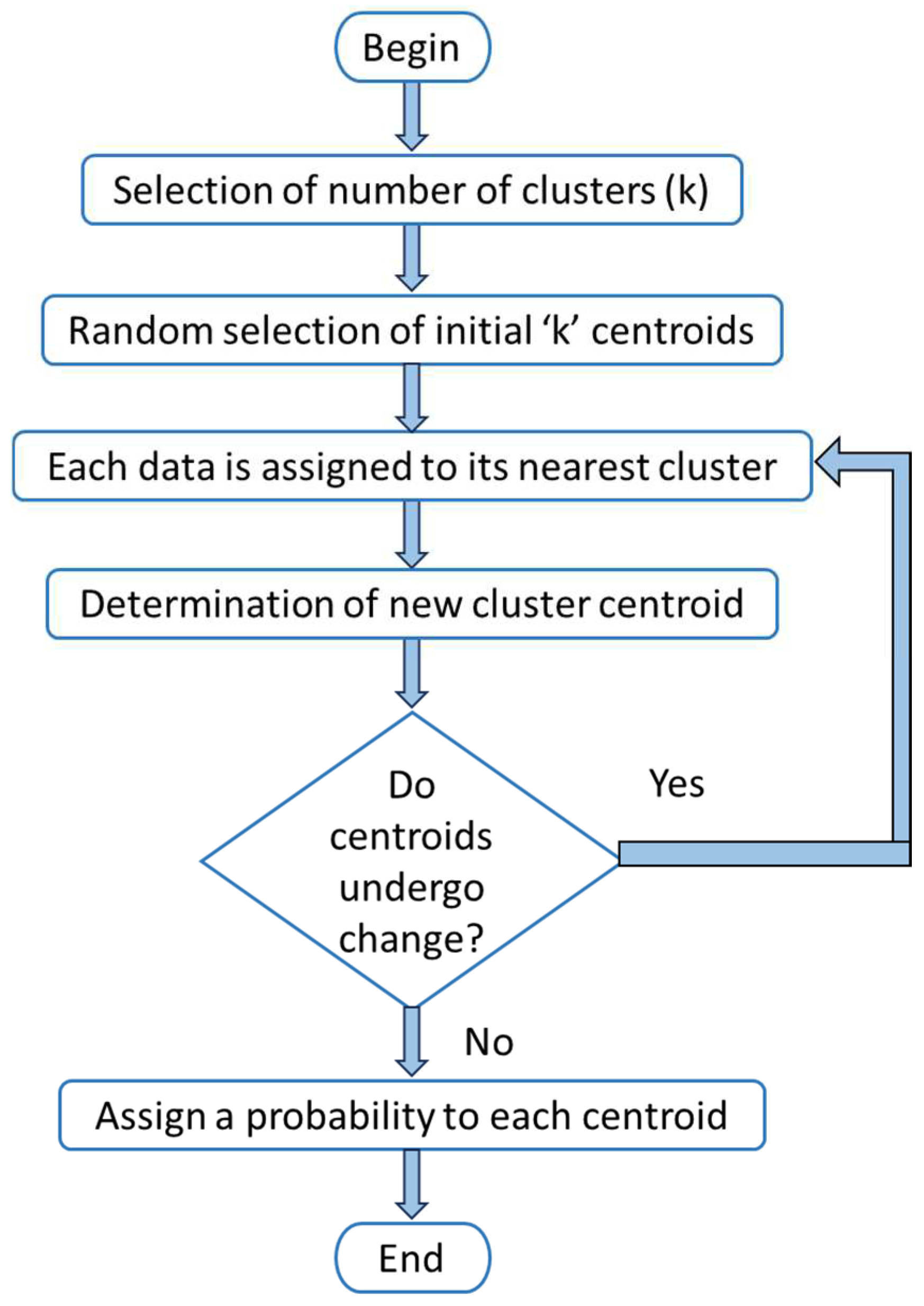
2.2.2. K-Means Technique

MCS is widely recognized as one of the most accurate and frequently employed probabilistic techniques for handling uncertainties. However, its application can be time-consuming for operators. Consequently, there has been a growing concern in recent years regarding the need for precise and efficient methods to model the stochastic nature of uncertainties. In response to this concern, the integration of several data mining methods into PSs studies is gaining considerable attention. Several clustering techniques, like fuzzy c-means [57], K-means [54,58], and adaptive K-means [59]; hierarchical clustering [60]; and K-medoids [58] have been employed by scholars. The renowned and accurate K-means clustering method was initially suggested by Mac Queen in 1967 [61], and it stands out due to its speed, efficiency, and simplicity. In the context of this study, the SCENRED is performed utilizing the K-means technique. The flowchart illustrating the K-means technique is presented in Figure 4 [54,62]. For a more comprehensive mathematical explanation of this technique, refer to [62].

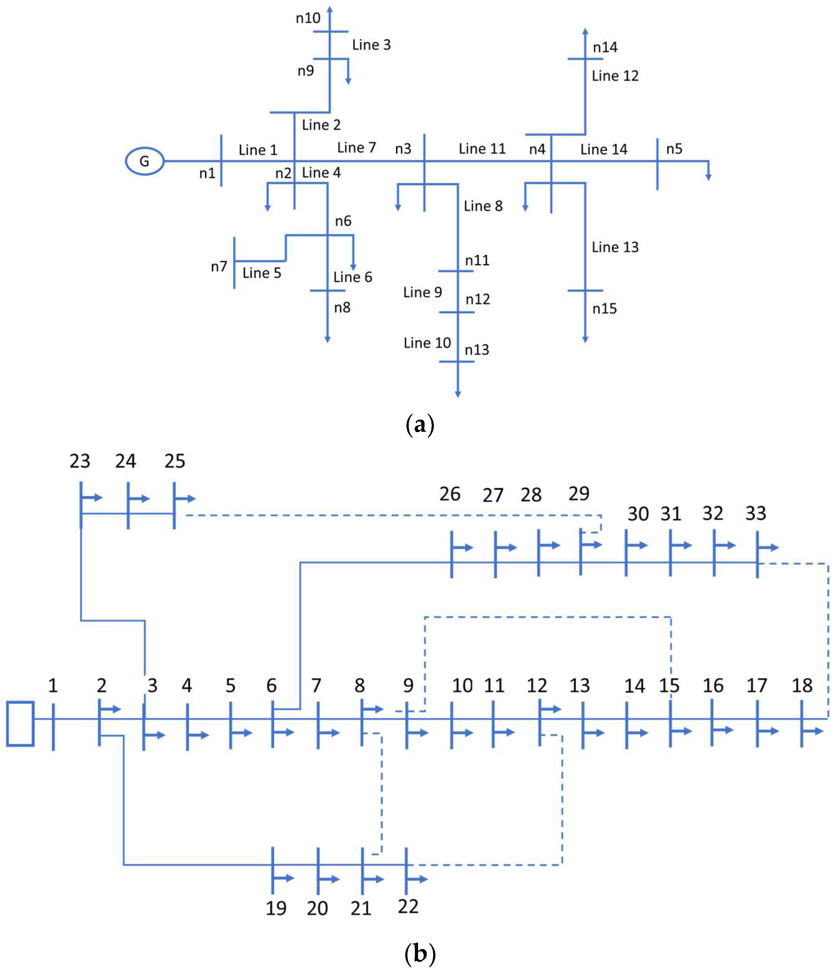
3. The Applications of DBN—IEEE 15 Bus System and IEEE 33 Bus System as Case Study

The performance of the proposed overhead line failure prediction model is evaluated on the IEEE 15 bus test network and IEEE 33 bus test network. These test systems are the standard benchmark systems and are widely used in resilience studies, therefore making them suitable for validating the proposed Dynamic Bayesian Network model. For an initial validation of the model, an IEEE 15 bus system is used. To further evaluate its effectiveness on a larger and more complex test system, an IEEE 33 bus system is used. The advantage of using a standard test system is that it facilitates other researchers too by easily reproducing and validating the results.

As stated earlier, generally, it is assumed that the system is exposed to the uniform weather conditions, and modeling is performed as a static event. However, in practice, power system (PS) grid lines encounter various Hurricane Wind Speed Intensity (HWSI) conditions across different times and environments [21] and is composed of several geographic regions [63]; therefore, in this study, to set up a disruptive event, both test systems have been affected by hurricanes of different categories. These events are modeled based on sustained wind speeds categorized according to the Saffir–Simpson Hurricane Wind Scale. It is the division of the US government’s National Oceanic and Atmospheric Administration (NOAA), the National Hurricane Center (NHC), which simulates sustained winds of various hurricane classifications based on the Saffir–Simpson Hurricane Wind Scale. These hurricanes are modeled as synchronous events. The wind speed range used in the study spans from Category 1 hurricanes (33–42.99 m/s) to Category 5 hurricanes (≥ 70 m/s). The analysis is conducted in a general framework, which is applicable to any distribution system; however, if needed, it can be adapted to specific geographical regions. The wind speed values used in the simulations are derived from well-established hurricane classifications, ensuring reliability with standard meteorological data.

The standard IEEE 15 bus radial distribution system [21] and IEEE 33 bus radial distribution system [63], shown in Figure 5a and Figure 5b, respectively, are implemented in this work as a case study. The hurricane wind speed affects the overhead powerline during its propagation. In this study, the impact of the HWSI at distinct times and locations on the grid are considered. The FP for the overhead power lines (due to failure of poles) in terms of failure stress (σ) of HWSI is computed using a DBN, and its comparison is made using the FC-MCS-SCENRED model. The objective is to calculate the probability of asset failure as time advances.

An overview of the proposed methodology is presented in Figure 6. The different stages of the methodology are detailed below.

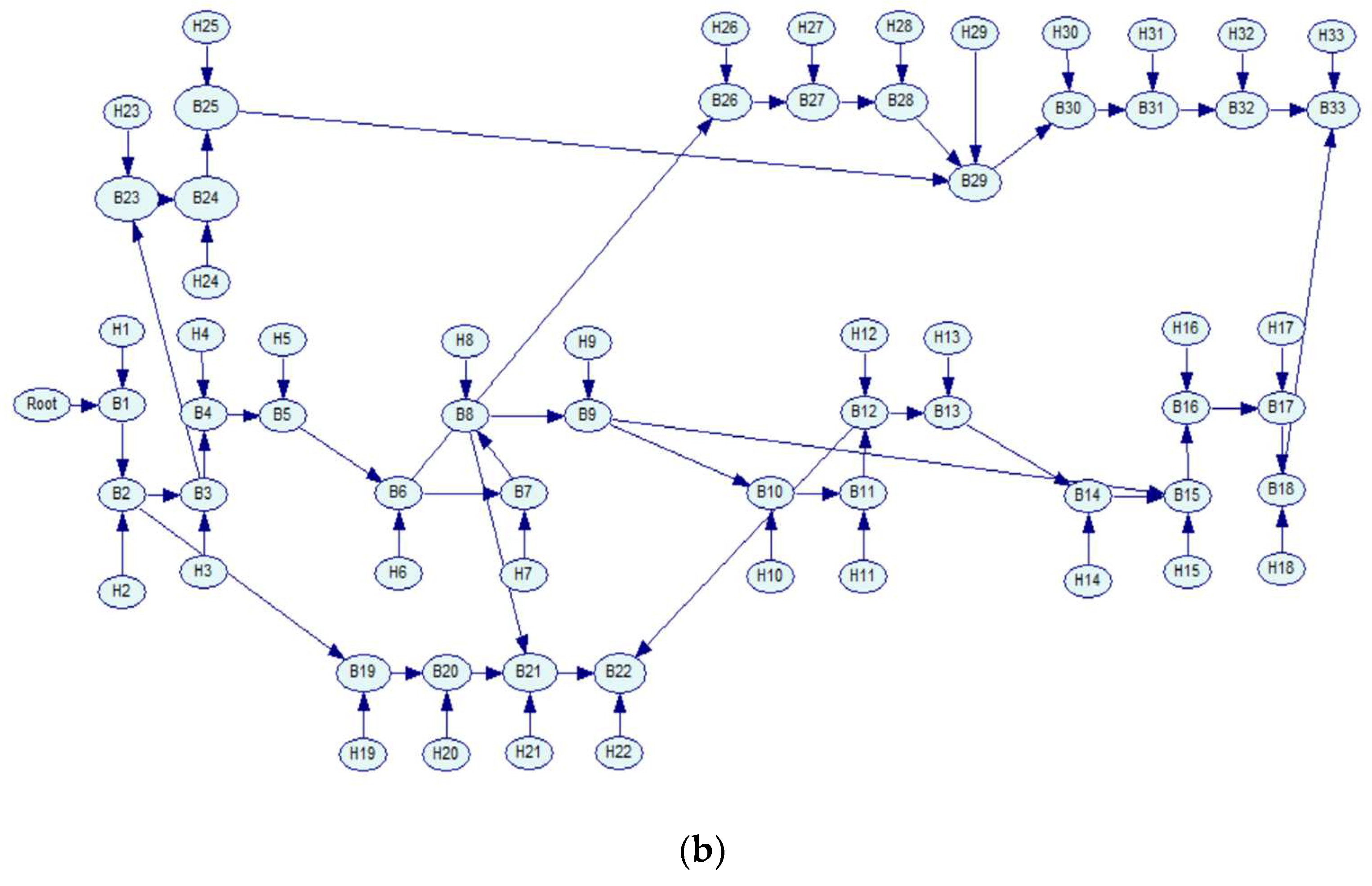
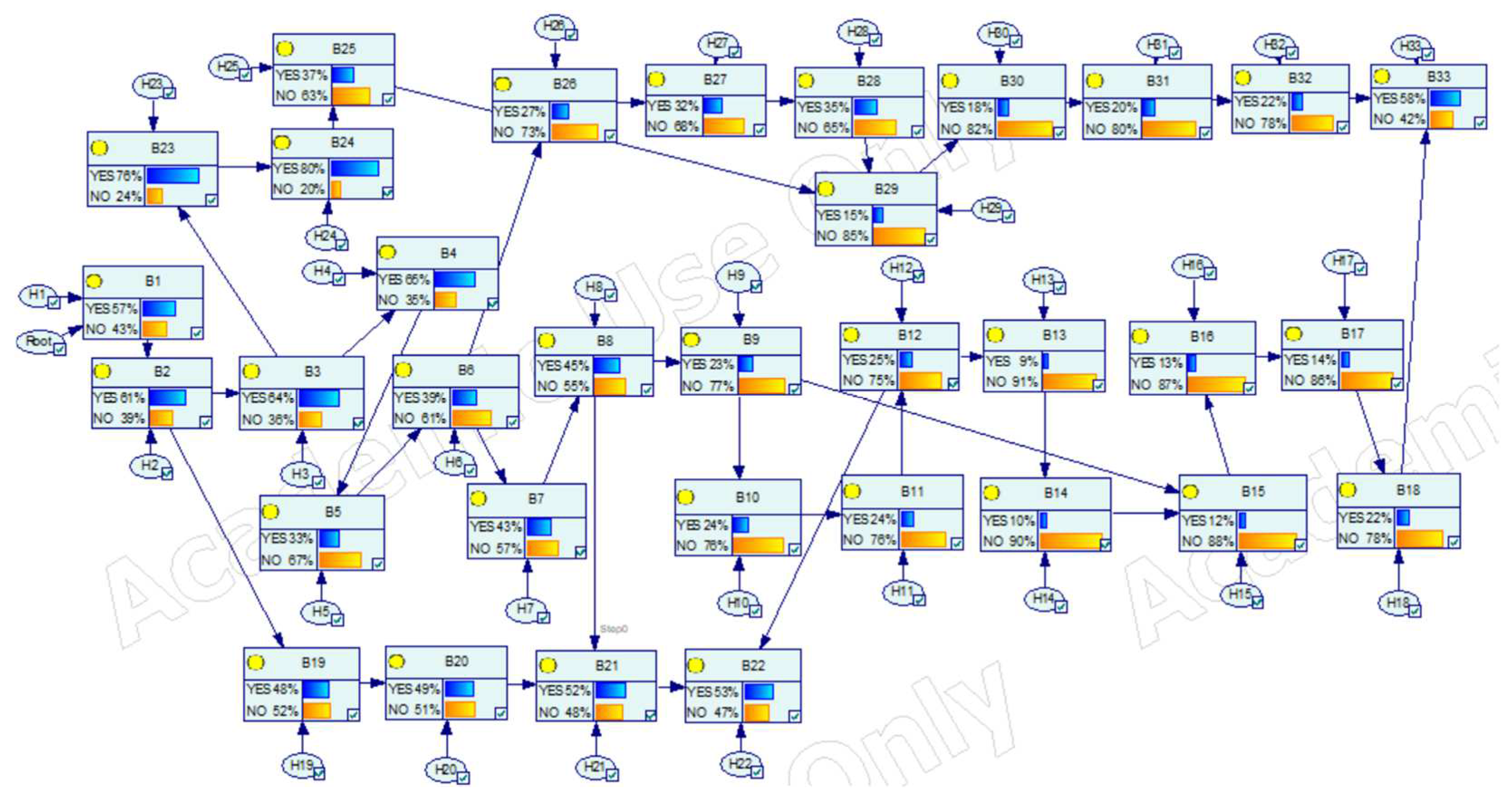
3.1. Step I: Creating a Bayesian Network (BN)

In step I, an initial qualitative BN model was formulated. This BN model was established by considering the impacts of hurricanes on distribution poles. This initial step led to the creation of a graphical model illustrating various parameters, the relationships between system poles, and the mechanisms associated with HIF.

Figure 7a,b depict a BN model for the standard IEEE 15 bus and IEEE 33 bus system, respectively, for overhead line failure estimation. In the model, the system nodes represent the random variable of the network, and the edge represents the causes of overhead line failure. A state $\mathrm{S}\mathrm{L}$ = 0 of $\mathrm{S}\mathrm{L}$ implies the line is out of service, and $\mathrm{S}\mathrm{L}$ = 1 implies the line is in service. The probability of line/pole falling is calculated depending upon the link between the poles and the HWSI. In Figure 7a, each child node in the BN model is dependent upon the two parent nodes, $\mathrm{S}\mathrm{L}$, and corresponding HWSI ($\mathrm{H}$). Therefore, the FP associated with any of these two ($\mathrm{S}\mathrm{L}$ or corresponding $\mathrm{H}$) will affect the FP status of the proceeding child $\mathrm{S}\mathrm{L}$. To compute this conditional dependence among various nodes, the marginal and the conditional probability tables (CPTs) of various nodes are defined with the help of parameter learning, as discussed in step II. The transmission of evidence from parent variables to child variables is termed as forecasting or prognosis, while the transmission of evidence from child variables to parent variables is referred to as inference or diagnosis [24].

3.2. Step II: Dynamic Framework for Overhead Lines

In step II, the constructed BN model of step I was converted to a dynamic probabilistic framework known as DBN. The software used as a tool to construct the DBN model was GeNIe [64]. DBN’s system nodes can be categorized into initial condition nodes and temporal plate nodes. The variables under the initial conditions category cover time-independent variables. That means such variables are static and not dynamic in nature. The variables under temporal plate category cover time-dependent variables. Such variables are said to be dynamic in nature. The risk event’s dynamic nature across time is reflected in the transition probability. Therefore, if λ and μ stand for the failure and repair rates, respectively; Δt for the time interval between the two time slices; and t for the current time, then the following is an expression for the transition probabilities of time-related nodes between two time slices [39]:

$$\mathrm{P}{(\mathrm{X}}_{\mathrm{t}+∆\mathrm{t}}^{\mathrm{i}}=0\left|{(\mathrm{X}}_{\mathrm{t}}^{\mathrm{i}}=0\right)={\mathrm{e}}^{-\mathsf{\lambda }∆\mathrm{t}}$$

(9a)

$$\mathrm{P}{(\mathrm{X}}_{\mathrm{t}+∆\mathrm{t}}^{\mathrm{i}}=1\left|{(\mathrm{X}}_{\mathrm{t}}^{\mathrm{i}}=0\right)={1-\mathrm{e}}^{-\mathsf{\lambda }∆\mathrm{t}}$$

(9b)

$$\mathrm{P}{(\mathrm{X}}_{\mathrm{t}+∆\mathrm{t}}^{\mathrm{i}}=0\left|{(\mathrm{X}}_{\mathrm{t}}^{\mathrm{i}}=1\right)={1-\mathrm{e}}^{-\mathsf{\mu }∆\mathrm{t}}$$

(9c)

$$\mathrm{P}{(\mathrm{X}}_{\mathrm{t}+∆\mathrm{t}}^{\mathrm{i}}=1\left|{(\mathrm{X}}_{\mathrm{t}}^{\mathrm{i}}=1\right)={\mathrm{e}}^{-\mathsf{\mu }∆\mathrm{t}}$$

(9d)

The transformation process from BN to DBN was accomplished in two distinct phases: (i) structural learning, which is associated with the configuration of the static BN, and (ii) parameter learning, which is associated with the probabilistic values. The first phase provided interdependencies or links among various nodes of the system and was the result of the first step. Through the second phase, the marginal and conditional probability tables (CPTs) of various variables or nodes were defined in the DBN. Each node was assigned probabilistic values ranging from 0 to 1 in the built structure of the BN model, based on expert’s opinion. In a DBN, the variables were considered to be varying with time. The prior probability distribution was therefore defined at the first-time step (t = 0), and the built DBN model was run for five time slices. This step resulted in the temporal BN model and provided us with the variation in nodes with respect to time.

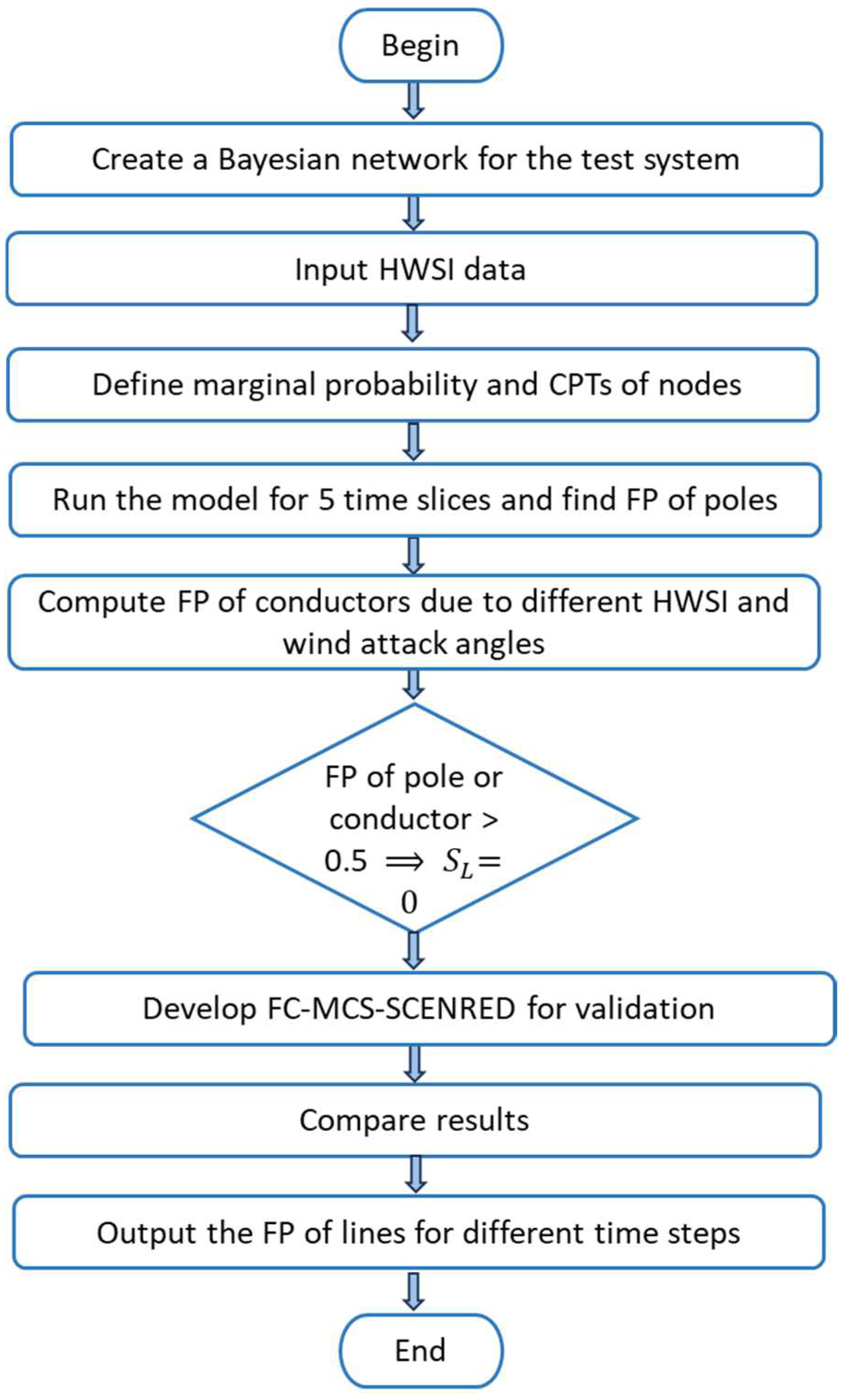
3.3. III: Bayesian Inference

In step III, the temporal characteristics of the DBN model acquired in the second step II were leveraged to perform Bayesian inference. Utilizing the GeNIe tool, we updated the probabilistic beliefs across five time steps, resulting in posterior probabilities for each variable within the BN model. It was assumed that the time slice in this study indicated a day; however, the time slice can be a second, a minute, an hour, a week, or any other duration depending upon the requirement [65]. Step III ultimately yielded the FP for overhead lines attributed to HWSI influence. In the proposed study, FP was understood as the likelihood of failure of assets due to the impact of HWSI.

3.4. Step IV: Validation Using FC-MCS-SCENRED Model

In step IV, the outcomes of step III were validated by using hybrid statistical probabilistic model called FC-MCS-SCENRED model. This step assisted in exploring the robustness and accuracy of the DBN model when predicting FP of the overhead lines due to HWSI. The FC-MCS-SCENRED model used for validation of DBN has been used in previous studies [21,66] as the most suitable means of validation for $\mathrm{S}\mathrm{L}$ outage prediction.

The FP for the poles in terms of failure stress (σ) of HWSI used in this study was adopted from [21] and is presented below:

$$\mathrm{F}\mathrm{P}\left(\mathsf{\sigma }\right)=1-{\mathrm{e}}^{-({\displaystyle \frac{\mathsf{\sigma }}{{\mathsf{\sigma }}_0}}{)}^{\mathrm{m}}}$$

(10)

where

$\mathrm{F}\mathrm{P}\left(\mathsf{\sigma }\right)$ is the probability of the electric pole failure in terms of stress (σ) of HWSI;

${\mathsf{\sigma }}_0$ is the reference stress;

$\mathrm{m}$ is the statistical Weibull modulus.

Using Equation (10), MCSs were performed to evaluate the FP for the poles due to rising HWSI. At each trial of MCS corresponding to line FP, a random number in the range 0 to 1 is generated. On comparing the generated number with the acquired line FP, if the number is found to be greater than the value of line FP, then it indicates that $\mathrm{S}\mathrm{L}=1$ and $\mathrm{S}\mathrm{L}=0$ if otherwise. It is important to emphasize that the failure of each of these poles can result in the failure of one or more additional poles within the system [40].

Capturing the uncertainties linked with the overhead line damage due to uncertain hurricane events is a necessary task, which is performed in this study using a scenario-based method. Depending on the historical data of HWSI, a probability distribution function (PDF) was established. Subsequently, a finite set of scenarios (1000 random scenarios) was generated via the MCS algorithm based on this PDF [53]. Then, the K-means SCENRED technique used in [54] was implemented here to reduce the number of scenarios from 1000 to 20 and then to 1 in a manner that kept the crucial details of the initial generated scenarios to the greatest extent possible. The flowchart illustrating the FC-MCS-SCENRED technique is presented in Figure 8.

The FC-MCS-SCENRED model outcomes were compared with the results of step III and are explained in the following section. The computation of failure probability of overhead lines is explained with the help of flowchart given in Figure 9.

4. Results and Discussion

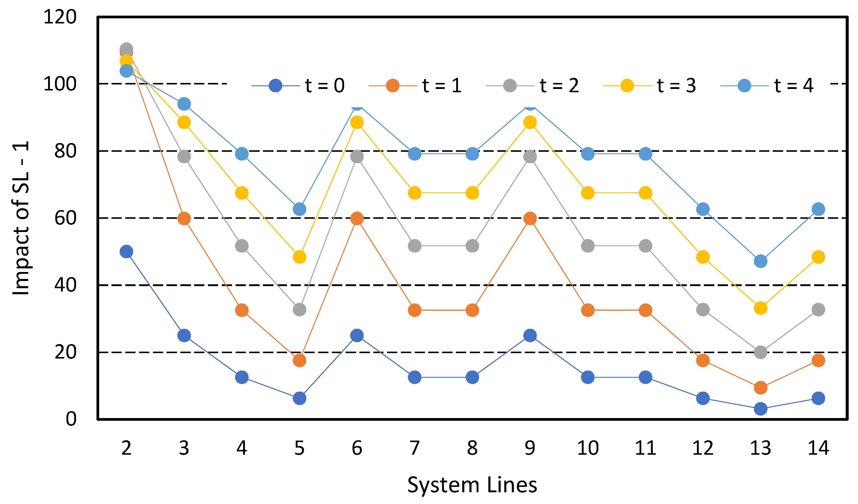
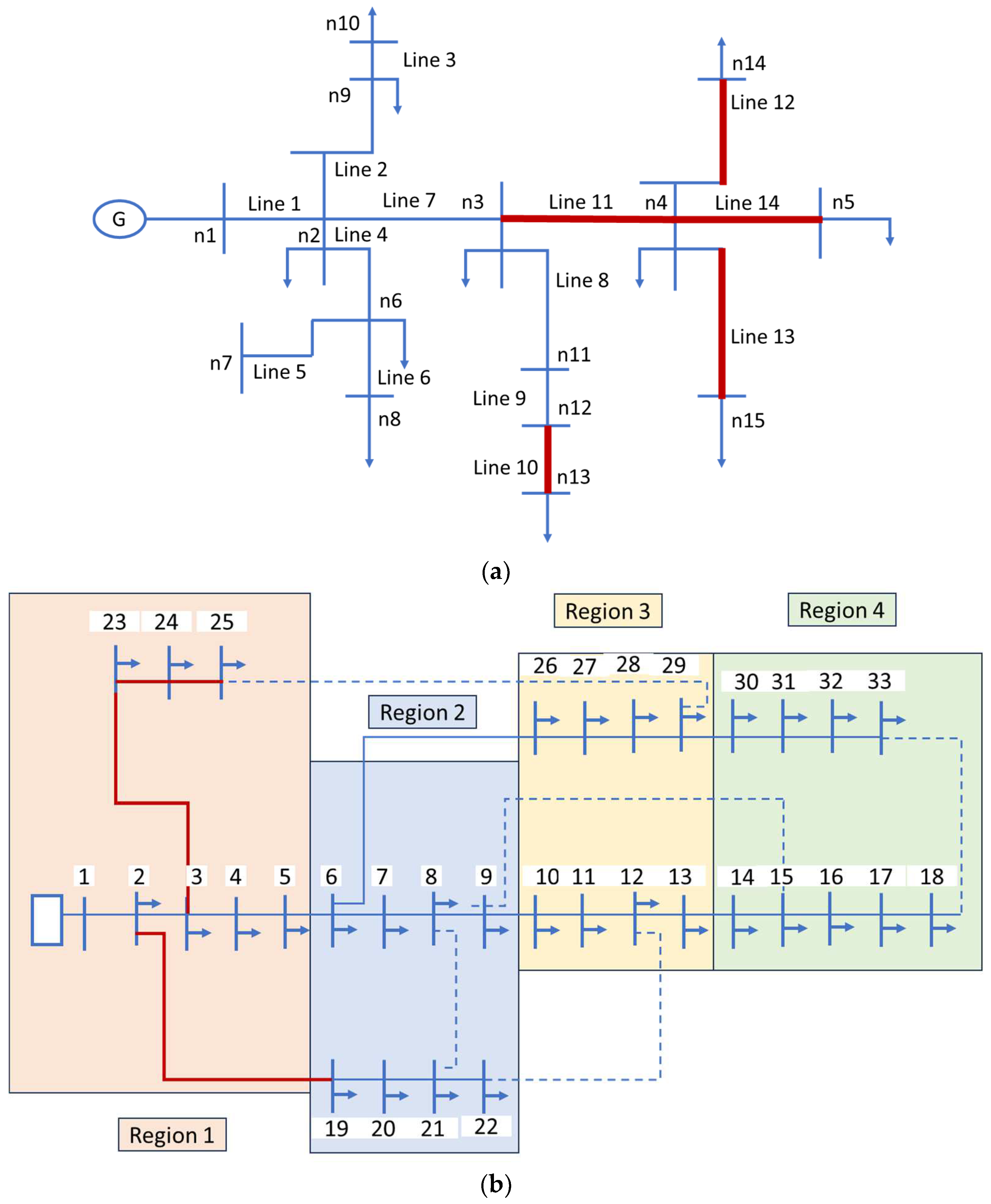
4.1. IEEE 15 Bus Test System

The IEEE 15 bus test system shown in Figure 5a is an 11 kV, 60 Hz radial distribution system [67]. The connection between different buses, representing a system line, is listed in

Table 1. Line outage prediction for IEEE 15 bus test system.

System Lines	From Bus—to Bus	HWSI	DBN		FC-MCS-SCENRED
		(m/s)	Failure Probability	Outage Prediction	Failure Probability	Outage Prediction
1	1−2	10.288	0.26	1	0	1
2	2−9	15.433	0.262	1	0.005	1
3	9−10	20.577	0.267	1	0.01	1
4	2−6	25.722	0.28	1	0.028	1
5	6−7	30.866	0.305	1	0.08	1
6	6−8	36.011	0.307	1	0.129	1
7	2−3	41.155	0.375	1	0.206	1
8	3−11	46.299	0.408	1	0.304	1
9	11−12	51.444	0.411	1	0.402	1
10	12−13	56.588	0.566	0	0.531	0
11	3−4	61.733	0.505	0	0.642	0
12	4−14	66.877	0.693	0	0.778	0
13	4−15	72.022	0.824	0	0.85	0
14	4−5	82.311	0.61	0	0.919	0

. Table 1 also enlists the sustained winds of different categories of hurricanes affecting the different poles and lines of the IEEE 15 bus test system.

Figure 10 shows the DBN simulation model results for the IEEE 15 bus test system. These results are obtained using GeNie 4. 0 Academic Software and indicate the failure probability of overhead $\mathrm{S}\mathrm{L}$ due to the failure of buses (poles). The blue bar of a variable with a “Yes” in Figure 10 indicates the FP percentage of a pole and an orange bar of a variable with a “No” in Figure 10 indicates the non-FP percentage of a pole. Each risk factor in Figure 8 ($\mathrm{B}$ or corresponding $\mathrm{H}$) has a PDF associated with it, representing the relative probability of that specific node. Depending on the state of the node, it may adopt a random value. In this model, the failure of $\mathrm{S}\mathrm{L}$ is considered due to the failure of the pole fiber. The arrows in Figure 10 signify the causal relationships, depicting the probabilistic connections between system risk factors that contribute to the FP of the asset. The probabilistic results of the system aid in exploring the detailed impact of the hurricane propagation profile, leading to asset failure with the passage of time.

Since the PS network is dynamic in nature, a practical scenario is investigated by running the simulation model in Figure 10 for over five time slices. To find out the dynamic FP of each $\mathrm{S}\mathrm{L}$, each $\mathrm{S}\mathrm{L}$ is hit simultaneously at t = 0 by a different intensity time-varying hurricane. The values of different HWSIs used are given in Table 1. In Figure 10, the simulation results for only one time slice along with their FP percentage is shown for clarity and convenience, while Figure 11 covers the simulation results for all five time slices.

From Figure 11, it can be clearly seen that for a particular $\mathrm{S}\mathrm{L}$, when the value of HWSI is low, i.e., initially for the low-order $\mathrm{S}\mathrm{L}$, each $\mathrm{S}\mathrm{L}$’s FP decreases with the increase in the order of time slices or the passage of time. However, as the HWSI progresses and goes beyond the $\mathrm{S}\mathrm{L}9$, the reverse trend in the dynamic probability is observed, i.e., the failure rate of a particular $\mathrm{S}\mathrm{L}$ for different time slices increases with the order of time slices. This point, after which the future FP trend changes (from decreasing to increasing) with respect to time slices, marks the threshold limit for the FP of the system, which in the case of the proposed DBN model is found to be 0.411 using GeNie software, as is clear from Table 1 and Figure 11. In the proposed DBN model, the line is therefore predicted to be broken from $\mathrm{S}\mathrm{L}10$ onwards when the 50% limit is exceeded. This 50% threshold value for $\mathrm{S}\mathrm{L}$ failure has also been adopted in studies [21,63]. This means that any $\mathrm{S}\mathrm{L}$ whose FP exceeds 50% (or 0.5) results in an outage, indicated by $\mathrm{S}\mathrm{L}$ status, $\mathrm{S}\mathrm{L}$ = 0.

Also, Figure 10 and Figure 11 show that for a particular value of time instant, the FP of consecutive $\mathrm{S}\mathrm{L}$ increases with the increase in HWSI depending upon the causal relationship. As can be seen from Figure 10 and Figure 11, among all the system lines, $\mathrm{S}\mathrm{L}13$ has the highest probability, while $\mathrm{S}\mathrm{L}1$ has the lowest probability for the five time slices even though $\mathrm{H}14$ is greater than $\mathrm{H}13$. That is, for the system line $\mathrm{S}\mathrm{L}14$, the FP is less than the FP of the system line $\mathrm{S}\mathrm{L}13$. However, since the corresponding $\mathrm{H}14$ is more than the $\mathrm{H}13$, the FP of $\mathrm{S}\mathrm{L}14$ should be more than the $\mathrm{S}\mathrm{L}13$, and $\mathrm{S}\mathrm{L}14$ should have the highest probability, like in the FC-MCS-SCENRED model. However, this is not found to be true in the case of the DBN because in the DBN, the effect of parent nodes and the causal relationship among variables is also considered. Since $\mathrm{S}\mathrm{L}13$ has $\mathrm{S}\mathrm{L}12$ as one of the two parent nodes, as shown in Figure 10, the FP is 69%, while the parent node of $\mathrm{S}\mathrm{L}14$, that is, $\mathrm{S}\mathrm{L}4$, has an FP of 28%. Since the FP of the two parent nodes is in the order of $\mathrm{S}\mathrm{L}12$ > $\mathrm{S}\mathrm{L}4$ and, therefore, so is the FP of their child nodes, $\mathrm{S}\mathrm{L}13$ > $\mathrm{S}\mathrm{L}14$ despite $\mathrm{H}14$ being greater than $\mathrm{H}13$, making $\mathrm{S}\mathrm{L}13$ the one with the highest FP. This shows that the HWSI and the causal relationship among lines has a direct influence on the future FP of $\mathrm{S}\mathrm{L}.$ The higher the HWSI and the FP of the parent line, the higher the future FP of a particular $\mathrm{S}\mathrm{L}$ and of consecutive lines and vice versa.

To investigate more about the causal relationship among lines, the same model runs over for five time slices again, but this time, each line is hit simultaneously by a fixed intensity hurricane of magnitude 10.288 m/s at the time instant t = 0, as shown in Figure 12. This is performed to avoid any effect due to varying magnitudes of HWSI for different lines. Since the same HWSI strikes all the lines s at t = 0, the initial FP of all the lines is the same (0.26). Also, it can be clearly seen in Figure 12 that for all the lines, a uniform pattern of the FP followed. Each line’s FP decreases with the increase in the order of time slices or with the passage of time, although the decrease in probability is not equal in magnitude. This difference in the decrease of the FP is because of different causal relationships among lines for later time instants (t = 1, 2, 3, and 4).

The causal relationship among system lines shown in Figure 12 is best illustrated with the help of the sensitivity analysis shown in Figure 13. Figure 13 shows how in a DBN model, the impact of the failure of $\mathrm{S}\mathrm{L}1$ has a cascading effect over the rest of the lines for different time instants. For instance, if the FP of $\mathrm{S}\mathrm{L}1$ at t = 0 is 1, then according to Figure 13, the FP of $\mathrm{S}\mathrm{L}2$ due to $\mathrm{S}\mathrm{L}1$ and $\mathrm{H}2$ at t = 0 will be 50% of the FP of $\mathrm{S}\mathrm{L}1$, the FP of $\mathrm{S}\mathrm{L}3$ due to $\mathrm{S}\mathrm{L}2$ and $\mathrm{H}3$ at t = 0 will be 25% of the FP of $\mathrm{S}\mathrm{L}1$, and so on. Figure 13 also shows how much of the percentage of the FP of $\mathrm{S}\mathrm{L}1$ the rest of the line’s FP will be if the FP of $\mathrm{S}\mathrm{L}1$ for t = 0, 1, 2, 3, and 4 is 1. As the failure rate of a power DS is based on the functional state of each pole, the failure rate is a time variant as well [24], as is evident from Figure 13.

As mentioned earlier, the line failure in a wind scenario could be due to the bending failure of poles or wire breakage. To model the line failure due to wire breakage, some parameters related to wind pressure calculation have been adopted from [68] due to the lack of design details. Therefore, assuming that the conductor is made up of an aluminum-conductor-steel-reinforced material (ACSR), the parameters adopted are the breaking strength of the ACSR wire = 406.5 Mpa.; the air density factor, ${\mathsf{\rho }}_{\mathrm{a}}=1$; the velocity pressure exposure coefficient for wire, ${\mathrm{k}}_{\mathrm{z}}$ = 1.1; the gust response factor of the wire, G = 0.88; and the force coefficient, ${\mathrm{C}}_{\mathrm{f}}$ = 1. Using these parameters, the wind pressure on the conductor span has been calculated for different wind attack angles ($\mathsf{\alpha }$) using Equation (3) and is shown in Figure 14.

From Figure 14, it has been found that as the HWSI increases, the wind pressure on the conductor also increases for a particular value of $\mathsf{\alpha }$. Also, the greater the $\mathsf{\alpha }$ is, the greater the wind pressure is on the conductor. This means that not only the HWSI but also the wind attack angle plays a crucial role in deciding the FP of a conductor. In this study, $\mathsf{\alpha }$ is taken to be equal to 30 degrees. Utilizing this information and Equation (2) for limit state function, the FP of the wire has been calculated. The FP is 0 if $\mathrm{R}<\mathrm{S}$ in the limit state function. From this graph, the lines found to be faulty include those corresponding to HWSI 61.733, 66.877, 72.022, and 82.311, for which the wind pressure on the conductor is more than that of the ACSR conductor (406.5 Mpa). Those faulty conductors are 11, 12, 13, and 14.

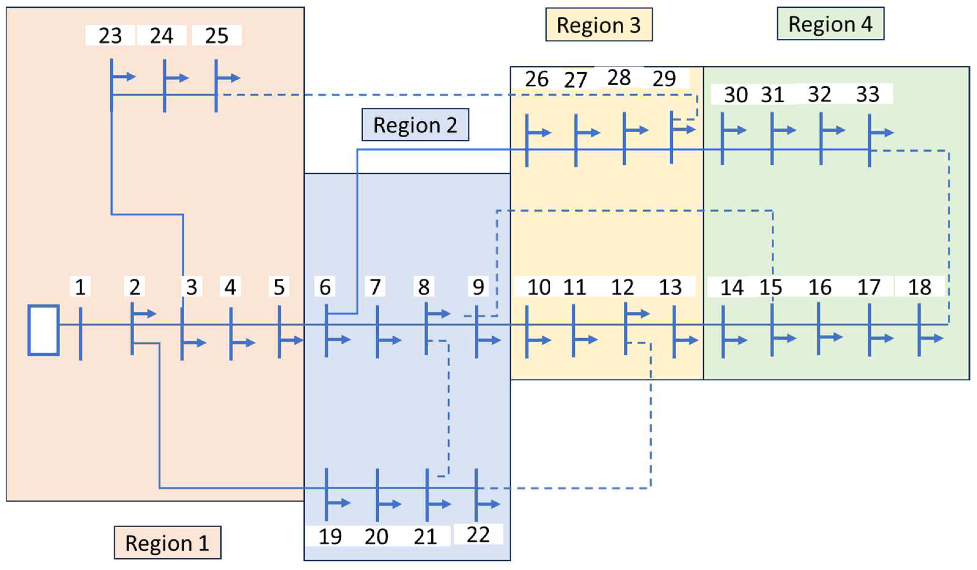
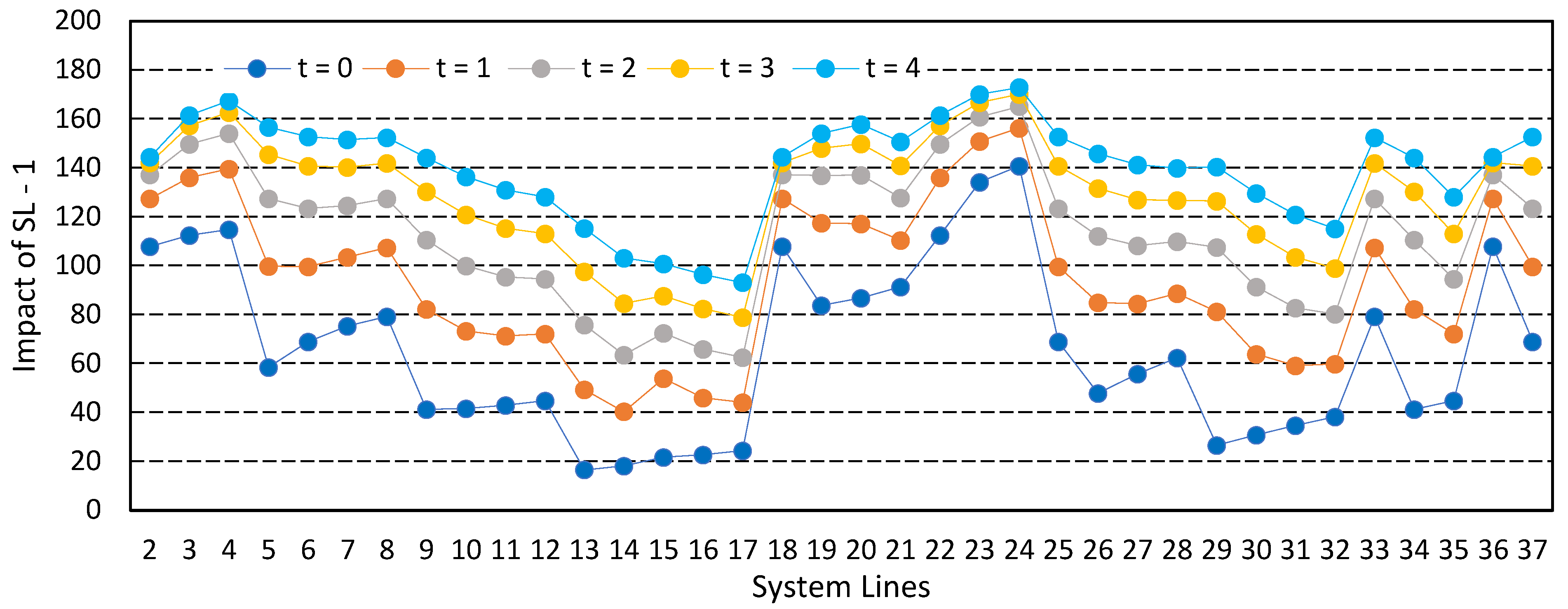
4.2. IEEE 33 Bus Test System

The IEEE 33 bus test system is a 12.66 kV distribution system with a reactive demand of 2300 kvar and an active demand of 3750 kW. It has thirty-two normally closed switches and five normally open switches [69]. The IEEE 33 bus test system has been divided into four regions based on the number of buses, as shown in Figure 15. Regions 1, 2, and 3 cover eight buses, while Region 4 covers nine buses. Regions 1, 2, 3, and 4 are affected by a hurricane category of 4, 3, 2, and 1, respectively. The different regions can have overlapping distribution lines, such as lines 5 and 18. The connection between different buses, representing a system line, is listed in

Table 2. Line outage prediction for IEEE 33 bus test system.

System Lines	From Bus—to Bus	HWSI	DBN		FC-MCS-SCENRED
		(m/s)	Failure Probability	Outage Prediction	Failure Probability	Outage Prediction
1	1−2	58.115	0.569	0	0.597	0
2	2−3	59.903	0.613	0	0.573	0
3	3−4	61.691	0.639	0	0.653	0
4	4−5	63.479	0.653	0	0.655	0
5	5−6	50.068	0.332	1	0.383	1
6	6−7	50.962	0.391	1	0.397	1
7	7−8	51.856	0.428	1	0.416	1
8	8−9	52.750	0.450	1	0.434	1
9	9−10	42.915	0.234	1	0.206	1
10	10−11	43.586	0.236	1	0.234	1
11	11−12	44.257	0.244	1	0.241	1
12	12−13	44.927	0.254	1	0.250	1
13	13−14	33.528	0.093	1	0.108	1
14	14−15	34.422	0.103	1	0.091	1
15	15−16	35.316	0.122	1	0.101	1
16	16−17	36.210	0.129	1	0.120	1
17	17−18	37.104	0.138	1	0.145	1
18	2−19	59.903	0.613	0	0.629	0
19	19−20	54.538	0.476	1	0.484	1
20	20−21	55.433	0.494	1	0.46	1
21	21−22	56.327	0.519	0	0.486	0
22	3−23	61.691	0.639	0	0.631	0
23	23−24	67.056	0.763	0	0.760	0
24	24−25	68.844	0.801	0	0.814	0
25	6−26	50.962	0.391	1	0.405	1
26	26−27	46.268	0.271	1	0.305	1
27	27−28	46.939	0.316	1	0.315	1
28	28−29	48.056	0.354	1	0.347	1
29	29−30	37.998	0.151	1	0.154	1
30	30−31	38.892	0.175	1	0.163	1
31	31−32	39.786	0.196	1	0.162	1
32	32−33	40.680	0.216	1	0.175	1
33	8−21	52.750	0.450	1	0.434	1
34	9−15	42.915	0.234	1	0.197	1
35	12−22	44.927	0.254	1	0.275	1
36	18−33	42.468	0.221	1	0.204	1
37	25−29	49.397	0.374	1	0.399	1

. Table 2 also enlists the sustained winds of different categories of hurricanes affecting the different poles and lines of the IEEE 33 bus test system.

Figure 16 shows the DBN simulation model results for the IEEE 33 bus test system. Like the previous case of IEEE 15 bus system, the model runs for over five time slices. Keeping in mind the clarity and convenience, in Figure 16, the simulation results for only one time slice along with the FP percentage of overhead $\mathrm{S}\mathrm{L}$ due to the failure of buses (poles) is shown, while Figure 17 covers the simulation results for all five time slices. To find out the dynamic FP of each $\mathrm{S}\mathrm{L}$, each $\mathrm{S}\mathrm{L}$ is hit simultaneously at t = 0 by a different intensity time-varying hurricane. The values of the different HWSIs used are given in Table 2.

From Figure 17, it can be clearly seen that for a particular $\mathrm{S}\mathrm{L}$ each $\mathrm{S}\mathrm{L}$’s FP for different time slices increases with the increase in time slices. This is like the FP trend of the IEEE 15 bus system beyond its $\mathrm{S}\mathrm{L}9$. It is to be noted that in the IEEE 33 bus system case, Regions 1, 2, 3, and 4 are affected by the category 4, 3, 2, and 1 hurricanes, respectively, unlike in the IEEE 15 bus system, where a reverse order of HWSI is adopted. Therefore, the FP trend for different time slices of an $\mathrm{S}\mathrm{L}$ for the two systems does not match exactly. In the proposed DBN model, the line is assumed to be broken when the 50% limit of the FP is exceeded. Also, Figure 16 and Figure 17 shows that for a particular value of time instant, the FP of consecutive $\mathrm{S}\mathrm{L}$ increases with the increase in HWSI depending upon the causal relationship. Among all the system lines, $\mathrm{S}\mathrm{L}24$ is found to have the highest FP, while $\mathrm{S}\mathrm{L}13$ has the lowest FP.

Figure 18 shows the sensitivity analysis for the IEEE 33 bus system. Figure 18 shows how in a DBN model the impact of failure of $\mathrm{S}\mathrm{L}1$ has a cascading effect over the rest of the lines for different time instants when the lines are hit by varying HWSI. For instance, if the FP of $\mathrm{S}\mathrm{L}1$ at t = 0 is 1, then according to Figure 18, the FP of $\mathrm{S}\mathrm{L}2$ due to $\mathrm{S}\mathrm{L}1$ and $\mathrm{H}2$ at t = 0 will be 107% of the FP of $\mathrm{S}\mathrm{L}1$, the FP of $\mathrm{S}\mathrm{L}3$ due to $\mathrm{S}\mathrm{L}2$ and $\mathrm{H}3$ at t = 0 will be 112% of the FP of $\mathrm{S}\mathrm{L}1$, and so on. It shows that the cascading effect progresses with time if the fault is not cleared timely.

Like the case of the IEEE 15 bus system, the wind pressure on the conductor span of the IEEE 33 bus system is also calculated for different wind attack angles ($\mathsf{\alpha }$) using Equation (3) and is shown in Figure 19. Figure 19 follows the same trend as in Figure 14, as the HWSI increases, the wind pressure on the conductor also increases for a particular value of $\mathsf{\alpha }$. Also, the greater the wind attack angle, $\mathsf{\alpha }$, is, the greater the wind pressure is on the conductor. From Figure 19, the lines found to be faulty include those corresponding to HWSI 58.115, 59.903, 61.691, 63.479, 59.903, 61.691, 67.056, and 68.844, for which the wind pressure on the conductor is more than that of the ACSR conductor (406.5 Mpa). Those faulty conductors are 1, 2, 3, 4, 18, 22, 23, and 24.

5. Model Validation

For both the test systems, the results are validated using the FC-MCS-SCENRED model used in [21] for the validation of the overhead line failure model. The results of the FC-MCS-SCENRED model for the IEEE 15 bus and IEEE 33 bus systems are presented as a heatmap in Figure 20 and Figure 21, respectively, for the one reduced scenario of the FP of $\mathrm{S}\mathrm{L}$. The dark colors in the heat map in the left-most column of Figure 20 indicate that for the lower-order SL corresponding to low HWSI, the FP is low. The FP increases with HWSI as we go from the left to the right column. For example, in Figure 20, it can be clearly seen that as the HWSI progresses with the $\mathrm{S}\mathrm{L}$, the FP of $\mathrm{S}\mathrm{L}$ also increases, and the status of the line changes from 1 to 0 from $\mathrm{S}\mathrm{L}10$ onwards as the FP exceeds 50%.

Similarly, in Figure 21, the dark colors corresponding to the low HWSI resulted in a low FP of $\mathrm{S}\mathrm{L}$. The FP increases with HWSI, as is evident from the yellow portion of the heatmap. In Figure 21, since the ascending HWSI is not applied to the sequential order of the system lines, rather than depending upon the regions, therefore, the FP is not seen increasing as we go from the left to the right column, as in Figure 20. For Figure 21, the $\mathrm{S}\mathrm{L}$ found to fail due to pole failure includes lines 1, 2, 3, 4, 18, 21, 22, 23, and 24. These failed lines are marked within the highlighted red rectangle in Figure 21.

A comparison between the DBN model and FC-MCS-SCENRED model is presented in Table 1 and Figure 22a for the IEEE 15 bus system and in Table 2 and Figure 22b for the IEEE 33 bus system. Table 1 and Table 2 prove that the DBN model $\mathrm{S}\mathrm{L}$ outage prediction results ($\mathrm{S}\mathrm{L}$ = 0 if line fails and $\mathrm{S}\mathrm{L}$ = 1 if otherwise) are consistent with the hybrid statistical probabilistic model (FC-MCS-SCENRED) of the DPSN component. The findings from this study can be utilized to create a maintenance schedule to mitigate HIF and to plan the grid proactively. It has been found that the change in the FP of an operational overhead line varies with HWSI. For example, in Table 1, when the HWSI is 10.288 m/s, the FP is found to be 0.26 and 0, while for an HWSI of 82.311 m/s, the FP is changed to 0.61 and 0.919 for the DBN and FC-MCS-SCENRED models, respectively. A 0 value obtained for the FP of FC-MCS-SCENRED is due to a low HWSI of 10.288 m/s, showing an almost negligible impact on the SL.

Figure 22a,b demonstrate that both the DBN model and FC-MCS-SCENRED model exhibit a similar FP trend over time. It reveals that in both models, the probability of a utility pole failure increases with HWSI affecting the $\mathrm{S}\mathrm{L}$. However, there are slight discrepancies between them, although these differences are relatively minor. The reason behind this could be the effect of parent nodes and the causal relationship among variables that are also considered in the DBN.

It is worth noting that the outcomes acquired from the DBN are derived from the structural learning of the DBN itself, primarily based on HWSI data. As such, they are considered to provide an approximate FP evaluation instead of an exact and precise one. In contrast, the outcomes from the FC-MCS-SCENRED model stem from a scenario-driven stochastic approach, which is widely regarded as a suitable means for validating $\mathrm{S}\mathrm{L}$ outage predictions, as mentioned in [48]. The comparative outcomes demonstrate that the DBN model can yield reliable and reasonable outcomes, like those obtained through the scenario-based stochastic approach. The graphical representation of the failed lines between different buses of the IEEE 15 and IEEE 33 bus test system due to both the failure of poles as well as conductors is shown in Figure 23a and Figure 23b by red color, respectively.

6. Conclusions

HIF in distribution overhead power lines poses severe risks to the PDSs. This study employs a DBN approach to model the HWSI mechanism on overhead distribution system. The network-based DBN approach, which incorporated interdependencies among the system variables, helps in understanding the HWSI as the key risk factor in the HIF mechanism that led to the failing of an overhead power line in the power distribution network. The study also concludes that as the HWSI progresses, it decreases the pole’s strength and significantly raises the FP and decreases the reliability of the asset. The same is true with wind attack angles and the conductor span. As the wind attack angle on the conductor increases, the wind pressure on the conductor increases and results in wire breakage more rapidly compared to low wind attack angles. Therefore, the higher the HWSI and wind attack angle is, the higher the FP of lines will be. The advantage of the proposed DBN-based model discussed in this study is that in addition to the current time instant, it predicts the FP of poles for the future time instant as well. Therefore, this in turn will help in taking proactive measures to reduce the risk of those failures and prevent a potential cascading failure in the network. This work holds potential for enhancing the reliability and maintenance scheduling of overhead power lines in the power industry, aiding in maintaining an FP within an adequate range and mitigating risks through regular maintenance.

As the network is susceptible to both unpredictable disruptions and deliberate attacks, the assessment of network resilience has become a critical aspect. Future work could integrate more complex models that include additional factors, such as the class and height of poles, the loads of fallen trees, etc., with the HIF DBN. This approach will provide valuable insights into identifying the risk factors that have the greatest economic impact on asset damage caused by high-impact events.

References

1. Stürmer, J.; Plietzsch, A.; Vogt, T.; Hellmann, F.; Kurths, J.; Otto, C.; Frieler, K.; Anvari, M. Protecting the Texas Power Grid from Tropical Cyclones: Increasing Resilience by Protecting Critical Lines. arXiv 2023, arXiv:2301.13793. [Google Scholar]
2. Daeli, A.; Mohagheghi, S. Power Grid Infrastructural Resilience against Extreme Events. Energies 2023, 16, 64. [Google Scholar] [CrossRef]
3. Liu, X.; Xie, Q.; Liang, H.; Zhang, X. Post-Earthquake Recover Strategy for Substations Based on Seismic Resilience Evaluation. Eng. Struct. 2023, 279, 115583. [Google Scholar] [CrossRef]
4. Salman, A.M.; Li, Y.; Stewart, M.G. Evaluating System Reliability and Targeted Hardening Strategies of Power Distribution Systems Subjected to Hurricanes. Reliab. Eng. Syst. Saf. 2015, 144, 319–333. [Google Scholar] [CrossRef]
5. Zhai, C.; Chen, T.Y.; White, A.G.; Guikema, S.D. Power Outage Prediction for Natural Hazards Using Synthetic Power Distribution Systems. Reliab. Eng. Syst. Saf. 2021, 208, 107348. [Google Scholar] [CrossRef]
6. Martinez-Amaya, J.; Radin, C.; Nieves, V. Advanced Machine Learning Methods for Major Hurricane Forecasting. Remote Sens. 2023, 15, 119. [Google Scholar] [CrossRef]
7. Klauberg, C.; Vogel, J.; Dalagnol, R.; Ferreira, M.P.; Hamamura, C.; Broadbent, E.; Silva, C.A. Post-Hurricane Damage Severity Classification at the Individual Tree Level Using Terrestrial Laser Scanning and Deep Learning. Remote Sens. 2023, 15, 1165. [Google Scholar] [CrossRef]
8. Cheng, P.-H.; Lin, C.C.-H.; Morton, Y.T.J.; Yang, S.-C.; Liu, J.-Y. A Bagged-Tree Machine Learning Model for High and Low Wind Speed Ocean Wind Retrieval From CYGNSS Measurements. IEEE Trans. Geosci. Remote Sens. 2023, 61, 1–10. [Google Scholar] [CrossRef]
9. Moeini, M.; Memari, A.M. Hurricane-Induced Failure Mechanisms in Low-Rise Residential Buildings and Future Research Directions. Nat. Hazards Rev. 2023, 24, 03123001. [Google Scholar] [CrossRef]
10. Faramarzi, D.; Rastegar, H.; Riahy, G.H.; Doagou-Mojarrad, H. A Three-Stage Hybrid Stochastic/IGDT Framework for Resilience-Oriented Distribution Network Planning. Int. J. Electr. Power Energy Syst. 2023, 146, 108738. [Google Scholar] [CrossRef]
11. McCann, Z.H.; Szaflarski, M. Differences in County-Level Cardiovascular Disease Mortality Rates Due to Damage Caused by Hurricane Matthew and the Moderating Effect of Social Capital: A Natural Experiment. BMC Public Health 2023, 23, 60. [Google Scholar] [CrossRef] [PubMed]
12. Liang, D.; Ewing, B.; Cardella, E.; Song, L. Probabilistic Modeling of Small Business Recovery after a Hurricane: A Case Study of 2017 Hurricane Harvey. Nat. Hazards Rev. 2023, 24, 05022012. [Google Scholar] [CrossRef]
13. Friedman, E.; Solecki, W.; Troxler, T.G.; Paganini, Z. Linking Quality of Life and Climate Change Adaptation Through the Use of the Macro-Adaptation Resilience Toolkit. Clim. Risk Manag. 2023, 39, 100485. [Google Scholar] [CrossRef]
14. Fatima, K.; Shareef, H.; Bajwa, A.A. An Insight into Power System Resilience and Its Confounding Traits. In Proceedings of the 2022 International Seminar on Application for Technology of Information and Communication (iSemantic), Semarang, Indonesia, 17–18 September 2022; pp. 226–231. [Google Scholar]
15. Xu, Y.; Xing, Y.; Huang, Q.; Li, J.; Zhang, G.; Bamisile, O.; Huang, Q. A Review of Resilience Enhancement Strategies in Renewable Power System under HILP Events. Energy Rep. 2023, 9, 200–209. [Google Scholar] [CrossRef]
16. Schmidt, D.H.; Garland, K.; Quebedeaux, L.K. Resilient Recovery Strategies: Lessons from the Local Nonprofit Sector Following Hurricane Ike. In Case Studies in Disaster Recovery; Elsevier: Amsterdam, The Netherlands, 2023; pp. 33–51. [Google Scholar]
17. Hou, G.; Muraleetharan, K.K.; Panchalogaranjan, V.; Moses, P.; Javid, A.; Al-Dakheeli, H.; Bulut, R.; Campos, R.; Harvey, P.S.; Miller, G. Resilience Assessment and Enhancement Evaluation of Power Distribution Systems Subjected to Ice Storms. Reliab. Eng. Syst. Saf. 2023, 230, 108964. [Google Scholar] [CrossRef]
18. Li, X.; Fu, D.; Nielsen-Gammon, J.; Gangrade, S.; Kao, S.C.; Chang, P.; Morales Hernández, M.; Voisin, N.; Zhang, Z.; Gao, H. Impacts of Climate Change on Future Hurricane Induced Rainfall and Flooding in a Coastal Watershed: A Case Study on Hurricane Harvey. J. Hydrol. 2023, 616, 128774. [Google Scholar] [CrossRef]
19. Darestani, Y.M.; Shafieezadeh, A. Multi-Dimensional Wind Fragility Functions for Wood Utility Poles. Eng. Struct. 2019, 183, 937–948. [Google Scholar] [CrossRef]
20. Panteli, M.; Mancarella, P. Influence of Extreme Weather and Climate Change on the Resilience of Power Systems: Impacts and Possible Mitigation Strategies. Electr. Power Syst. Res. 2015, 127, 259–270. [Google Scholar] [CrossRef]
21. Omogoye, O.S.; Folly, K.A.; Awodele, K.O. Enhancing the Distribution Power System Resilience against Hurricane Events Using a Bayesian Network Line Outage Prediction Model. J. Eng. 2021, 2021, 731–744. [Google Scholar] [CrossRef]
22. Fatima, K.; Sefid, M.; Anees, M.A.; Rihan, M. An Investigation of the Impact of Synchrophasors Measurement on Multi-Area State Estimation in Active Distribution Grids. Aust. J. Electr. Electron. Eng. 2020, 17, 122–131. [Google Scholar] [CrossRef]
23. Jiang, S.; Yang, L.; Cheng, G.; Gao, X.; Feng, T.; Zhou, Y. A Quantitative Framework for Network Resilience Evaluation Using Dynamic Bayesian Network. Comput. Commun. 2022, 194, 387–398. [Google Scholar] [CrossRef]
24. Lu, Q.; Zhang, W. Integrating Dynamic Bayesian Network and Physics-Based Modeling for Risk Analysis of a Time-Dependent Power Distribution System during Hurricanes. Reliab. Eng. Syst. Saf. 2022, 220, 108290. [Google Scholar] [CrossRef]
25. Shafieezadeh, A.; Onyewuchi, U.P.; Begovic, M.M.; DesRoches, R. Age-dependent fragility models of utility wood poles in power distribution networks against extreme wind hazards. IEEE Trans. Power Del. 2013, 29, 131–139. [Google Scholar]
26. Winkler, J.; Duenas-Osorio, L.; Stein, R.; Subramanian, D. Performance Assessment of Topologically Diverse Power Systems Subjected to Hurricane Events. Reliab. Eng. Syst. Saf. 2010, 95, 323–336. [Google Scholar] [CrossRef]
27. Ouyang, M.; Duenas-Osorio, L. Multi-Dimensional Hurricane Resilience Assessment of Electric Power Systems. Struct. Saf. 2014, 48, 15–24. [Google Scholar] [CrossRef]
28. Hughes, W.; Zhang, W.; Cerrai, D.; Bagtzoglou, A.; Wanik, D.; Anagnostou, E. A Hybrid Physics-Based and Data-Driven Model for Power Distribution System Infrastructure Hardening and Outage Simulation. Reliab. Eng. Syst. Saf. 2022, 225, 108628. [Google Scholar] [CrossRef]
29. Kammouh, O.; Gardoni, P.; Cimellaro, G.P. Probabilistic Framework to Evaluate the Resilience of Engineering Systems Using Bayesian and Dynamic Bayesian Networks. Reliab. Eng. Syst. Saf. 2020, 198, 106813. [Google Scholar] [CrossRef]
30. Hou, H.; Zhang, Z.; Wei, R.; Huang, Y.; Liang, Y.; Li, X. Review of Failure Risk and Outage Prediction in Power System under Wind Hazards✰. Electr. Power Syst. Res. 2022, 210, 108098. [Google Scholar] [CrossRef]
31. Fatima, K.; Shareef, H.; Costa, F.B.; Bajwa, A.A.; Wong, L.A. Machine Learning for Power Outage Prediction during Hurricanes: An Extensive Review. Eng. Appl. Artif. Intell. 2024, 133, 108056. [Google Scholar] [CrossRef]
32. Nateghi, R.; Guikema, S.; Quiring, S.M. Power Outage Estimation for Tropical Cyclones: Improved Accuracy with Simpler Models. Risk Anal. 2014, 34, 1069–1078. [Google Scholar] [CrossRef]
33. Hou, H.; Zhang, Z.; Yu, J.; Wei, R.; Huang, Y.; Li, X. Damage Prediction of 10 KV Power Towers in Distribution Network under Typhoon Disaster Based on Data-Driven Model. Int. J. Electr. Power Energy Syst. 2022, 142, 108307. [Google Scholar] [CrossRef]
34. Kankanala, P.; Das, S.; Pahwa, A. AdaBoost+: An Ensemble Learning Approach for Estimating Weather-Related Outages in Distribution Systems. IEEE Trans. Power Syst. 2014, 29, 359–367. [Google Scholar] [CrossRef]
35. Udeh, K.; Wanik, D.W.; Cerrai, D.; Aguiar, D.; Anagnostou, E. Autoregressive Modeling of Utility Customer Outages with Deep Neural Networks. In Proceedings of the 2022 IEEE 12th Annual Computing and Communication Workshop and Conference (CCWC), Las Vegas, NV, USA, 26–29 January 2022; pp. 406–414. [Google Scholar]
36. Khediri, A.; Laouar, M.R. Deep-Belief Network Based Prediction Model for Power Outage in Smart Grid. In Proceedings of the 4th ACM International Conference of Computing for Engineering and Sciences, Kuala Lumpur, Malaysia, 6–8 July 2018; pp. 1–6. [Google Scholar]
37. Yang, F.; Watson, P.; Koukoula, M.; Anagnostou, E.N. Enhancing Weather-Related Power Outage Prediction by Event Severity Classification. IEEE Access 2020, 8, 60029–60042. [Google Scholar] [CrossRef]
38. Ryan, P.C.; Stewart, M.G.; Spencer, N.; Li, Y. Reliability Assessment of Power Pole Infrastructure Incorporating Deterioration and Network Maintenance. Reliab. Eng. Syst. Saf. 2014, 132, 261–273. [Google Scholar] [CrossRef]
39. Guo, Y.; Wang, H.; Guo, Y.; Zhong, M.; Li, Q.; Gao, C. System Operational Reliability Evaluation Based on Dynamic Bayesian Network and XGBoost. Reliab. Eng. Syst. Saf. 2022, 225, 108622. [Google Scholar] [CrossRef]
40. Khomami, M.S.; Sepasian, M.S. Pre-Hurricane Optimal Placement Model of Repair Teams to Improve Distribution Network Resilience. Electr. Power Syst. Res. 2018, 165, 1–8. [Google Scholar] [CrossRef]
41. Yang, Y.; Khan, F.; Thodi, P.; Abbassi, R. Corrosion Induced Failure Analysis of Subsea Pipelines. Reliab. Eng. Syst. Saf. 2017, 159, 214–222. [Google Scholar] [CrossRef]
42. Sajid, Z.; Khan, F.; Zhang, Y. Integration of Interpretive Structural Modelling with Bayesian Network for Biodiesel Performance Analysis. Renew. Energy 2017, 107, 194–203. [Google Scholar] [CrossRef]
43. Taleb-Berrouane, M.; Khan, F.; Hawboldt, K. Corrosion Risk Assessment Using Adaptive Bow-Tie (ABT) Analysis. Reliab. Eng. Syst. Saf. 2021, 214, 107731. [Google Scholar] [CrossRef]
44. Adumene, S.; Khan, F.; Adedigba, S.; Zendehboudi, S. Offshore System Safety and Reliability Considering Microbial Influenced Multiple Failure Modes and Their Interdependencies. Reliab. Eng. Syst. Saf. 2021, 215, 107862. [Google Scholar] [CrossRef]
45. Khakzad, N.; Khan, F.; Amyotte, P. Safety Analysis in Process Facilities: Comparison of Fault Tree and Bayesian Network Approaches. Reliab. Eng. Syst. Saf. 2011, 96, 925–932. [Google Scholar] [CrossRef]
46. Taleb-Berrouane, M.; Khan, F.; Hawboldt, K.; Eckert, R.; Skovhus, T.L. Model for Microbiologically Influenced Corrosion Potential Assessment for the Oil and Gas Industry. Corros. Eng. Sci. Technol. 2018, 53, 378–392. [Google Scholar] [CrossRef]
47. Bensi, M.; Der Kiureghian, A.; Straub, D. Efficient Bayesian Network Modeling of Systems. Reliab. Eng. Syst. Saf. 2013, 112, 200–213. [Google Scholar] [CrossRef]
48. Hassan, S.; Wang, J.; Kontovas, C.; Bashir, M. An Assessment of Causes and Failure Likelihood of Cross-Country Pipelines under Uncertainty Using Bayesian Networks. Reliab. Eng. Syst. Saf. 2022, 218, 108171. [Google Scholar] [CrossRef]
49. Moradi, R.; Cofre-Martel, S.; Lopez Droguett, E.; Modarres, M.; Groth, K.M. Integration of Deep Learning and Bayesian Networks for Condition and Operation Risk Monitoring of Complex Engineering Systems. Reliab. Eng. Syst. Saf. 2022, 222, 108433. [Google Scholar] [CrossRef]
50. Dao, U.; Sajid, Z.; Khan, F.; Zhang, Y. Dynamic Bayesian Network Model to Study Under-Deposit Corrosion. Reliab. Eng. Syst. Saf. 2023, 237, 109370. [Google Scholar] [CrossRef]
51. Sajid, Z. A Dynamic Risk Assessment Model to Assess the Impact of the Coronavirus (COVID-19) on the Sustainability of the Biomass Supply Chain: A Case Study of a U.S. Biofuel Industry. Renew. Sustain. Energy Rev. 2021, 151, 111574. [Google Scholar] [CrossRef]
52. Sajid, Z.; Khan, F.; Veitch, B. Dynamic Ecological Risk Modelling of Hydrocarbon Release Scenarios in Arctic Waters. Mar. Pollut. Bull. 2020, 153, 111001. [Google Scholar] [CrossRef]
53. Rezaei, N.; Pezhmani, Y. Optimal Islanding Operation of Hydrogen Integrated Multi-Microgrids Considering Uncertainty and Unexpected Outages. J. Energy Storage 2022, 49, 104142. [Google Scholar] [CrossRef]
54. Rezaei, N.; Pezhmani, Y.; Mohammadiani, R.P. Optimal Stochastic Self-Scheduling of a Water-Energy Virtual Power Plant Considering Data Clustering and Multiple Storage Systems. J. Energy Storage 2023, 65, 107366. [Google Scholar] [CrossRef]
55. Taheri, B.; Safdarian, A.; Moeini-Aghtaie, M.; Lehtonen, M. Enhancing Resilience Level of Power Distribution Systems Using Proactive Operational Actions. IEEE Access 2019, 7, 137378–137389. [Google Scholar] [CrossRef]
56. Poudel, S.; Dubey, A.; Bose, A. Risk-Based Probabilistic Quantification of Power Distribution System Operational Resilience. IEEE Syst. J. 2020, 14, 3506–3517. [Google Scholar] [CrossRef]
57. Zhou, K.; Yang, S.; Shao, Z. Household Monthly Electricity Consumption Pattern Mining: A Fuzzy Clustering-Based Model and a Case Study. J. Clean. Prod. 2017, 141, 900–908. [Google Scholar] [CrossRef]
58. McLoughlin, F.; Duffy, A.; Conlon, M. A Clustering Approach to Domestic Electricity Load Profile Characterisation Using Smart Metering Data. Appl. Energy 2015, 141, 190–199. [Google Scholar] [CrossRef]
59. Wang, Y.; Chen, Q.; Kang, C.; Xia, Q. Clustering of Electricity Consumption Behavior Dynamics Toward Big Data Applications. IEEE Trans. Smart Grid 2016, 7, 2437–2447. [Google Scholar] [CrossRef]
60. Ozawa, A.; Furusato, R.; Yoshida, Y. Determining the Relationship between a Household’s Lifestyle and Its Electricity Consumption in Japan by Analyzing Measured Electric Load Profiles. Energy Build. 2016, 119, 200–210. [Google Scholar] [CrossRef]
61. MacQueen, J. Some Methods for Classification and Analysis of Multivariate Observations. In Proceedings of the Fifth Berkeley Symposium on Mathematical Statistics and Probability, Oakland, CA, USA, 1 January 1967; Volume 1, pp. 281–297. [Google Scholar]
62. Galvani, S.; Rezaeian Marjani, S.; Morsali, J.; Ahmadi Jirdehi, M. A New Approach for Probabilistic Harmonic Load Flow in Distribution Systems Based on Data Clustering. Electr. Power Syst. Res. 2019, 176, 105977. [Google Scholar] [CrossRef]
63. Bajwa, A.A.; Mokhlis, H.; Mekhlief, S.; Mubin, M.; Azam, M.M.; Sarwar, S. Resilience-Oriented Service Restoration Modelling Interdependent Critical Loads in Distribution Systems with Integrated Distributed Generators. IET Gener. Transm. Distrib. 2021, 15, 1257–1272. [Google Scholar] [CrossRef]
64. GeNIe Modeler by BayesFusion, LLC. Available online: https://www.bayesfusion.com/genie/ (accessed on 2 February 2024).
65. Yazdi, M.; Khan, F.; Abbassi, R.; Quddus, N. Resilience Assessment of a Subsea Pipeline Using Dynamic Bayesian Network. J. Pipeline Sci. Eng. 2022, 2, 100053. [Google Scholar] [CrossRef]
66. Omogoye, O.S.; Folly, K.A.; Awodele, K.O. Review of Proactive Operational Measures for the Distribution Power System Resilience Enhancement Against Hurricane Events. In Proceedings of the 2021 Southern African Universities Power Engineering Conference/Robotics and Mechatronics/Pattern Recognition Association of South Africa (SAUPEC/RobMech/PRASA), Potchefstroom, South Africa, 27–29 January 2021; pp. 1–6. [Google Scholar]
67. Naik, V.K.; Yadav, A. High Impedance Fault Detection and Classification on IEEE-15 Bus Radial Distribution System by Using Fuzzy Inference System. In Proceedings of the 2018 2nd International Conference on Power, Energy and Environment: Towards Smart Technology (ICEPE), Shillong, India, 1–2 June 2018; pp. 1–6. [Google Scholar]
68. Hou, G.; Muraleetharan, K.K. Modeling the Resilience of Power Distribution Systems Subjected to Extreme Winds Considering Tree Failures: An Integrated Framework. Int. J. Disaster Risk Sci. 2023, 14, 194–208. [Google Scholar] [CrossRef]
69. Muhammad, M.A.; Mokhlis, H.; Naidu, K.; Amin, A.; Franco, J.F.; Othman, M. Distribution Network Planning Enhancement via Network Reconfiguration and DG Integration Using Dataset Approach and Water Cycle Algorithm. J. Mod. Power Syst. Clean Energy 2020, 8, 86–93. [Google Scholar] [CrossRef]
Figure 1. POP exploiting various categories of (a) modern learning approach (b) machine learning algorithms [31].
Forecasting 07 00011 g001
Figure 2. A static BN showing the root node ( X 1 0 ) , the intermediate nodes ( X 2 0 and X 3 0 ), and the leaf node ( X 4 0 ).
Forecasting 07 00011 g002
Figure 3. A graphical representation of a DBN over N time slices.
Forecasting 07 00011 g003
Figure 4. Flowchart for K-means SCENRED technique.
Forecasting 07 00011 g004
Figure 5. The standard radial test distribution system: (a) IEEE 15 bus and (b) IEEE 33 bus.
Forecasting 07 00011 g005
Figure 6. An illustrative representation of the methodology used in the case study.
Forecasting 07 00011 g006
Figure 7. The structure of the BN overhead line outage prediction model: (a) IEEE 15 bus system and (b) IEEE 33 bus system.
Forecasting 07 00011 g007aForecasting 07 00011 g007b
Figure 8. Flowchart for FC-MCS-SCENRED technique.
Forecasting 07 00011 g008
Figure 9. Flowchart for determining failure probability of overhead system line using DBN.
Forecasting 07 00011 g009
Figure 10. DBN simulation model for IEEE 15 bus overhead S L failure.
Forecasting 07 00011 g010
Figure 11. Dynamic FP of each S L for different HWSIs over 5 time slices for IEEE 15 bus system.
Forecasting 07 00011 g011
Figure 12. Dynamic FP of each S L for same HWSI over 5 time slices.
Forecasting 07 00011 g012
Figure 13. The sensitivity analysis—the impact of S L 1 on the consecutive system lines of the IEEE 15 bus system.
Forecasting 07 00011 g013
Figure 14. Wind pressure on conductors of IEEE bus system for different wind attack angles and HWSI.
Forecasting 07 00011 g014
Figure 15. Regional set up: IEEE 33 bus radial distribution system.
Forecasting 07 00011 g015
Figure 16. DBN simulation model for IEEE 33 bus overhead S L failure.
Forecasting 07 00011 g016
Figure 17. Dynamic FP of each S L for different HWSI over 5 time slices for IEEE 33 bus system.
Forecasting 07 00011 g017
Figure 18. The sensitivity analysis—the impact of S L 1 on the consecutive system lines of the IEEE 33 bus system.
Forecasting 07 00011 g018
Figure 19. Wind pressure on conductors of the IEEE 33 bus system for different wind attack angles and HWSIs.
Forecasting 07 00011 g019
Figure 20. Damage scenarios of FC-MCS-SCENRED model for IEEE 15 bus system.
Forecasting 07 00011 g020
Figure 21. Damage scenarios of FC-MCS-SCENRED model for IEEE 33 bus system.
Forecasting 07 00011 g021
Figure 22. SL FP using DBN and FC-MCS-SCENRED for different HWSI: (a) IEEE 15 bus system and (b) IEEE 33 bus system.
Forecasting 07 00011 g022
Figure 23. The graphical representation of the line faults on standard radial distribution systems: the (a) IEEE 15 bus system and (b) IEEE 33 bus system.
Forecasting 07 00011 g023