Abstract
This study investigates wind speed prediction using advanced machine learning techniques, comparing the performance of Vanilla long short-term memory (LSTM) and convolutional neural network (CNN) models, alongside the application of extreme value theory (EVT) using the r-largest order generalised extreme value distribution (). Over the past couple of decades, the academic literature has transitioned from conventional statistical time series models to embracing EVT and machine learning algorithms for the modelling of environmental variables. This study adds value to the literature and knowledge of modelling wind speed using both EVT and machine learning. The primary aim of this study is to forecast wind speed in the Limpopo province of South Africa to showcase the dependability and potential of wind power generation. The application of CNN showcased considerable predictive accuracy compared to the Vanilla LSTM, achieving 88.66% accuracy with monthly time steps. The CNN predictions for the next five years, in m/s, were 9.91 (2024), 7.64 (2025), 7.81 (2026), 7.13 (2027), and 9.59 (2028), slightly outperforming the Vanilla LSTM, which predicted 9.43 (2024), 7.75 (2025), 7.85 (2026), 6.87 (2027), and 9.43 (2028). This highlights CNN’s superior ability to capture complex patterns in wind speed dynamics over time. Concurrently, the analysis of the across various order statistics identified as the optimal model, supported by its favourable evaluation metrics in terms of Akaike information criteria (AIC) and Bayesian information criteria (BIC). The 300-year return level for was found to be 22.89 m/s, indicating a rare wind speed event. Seasonal wind speed analysis revealed distinct patterns, with winter emerging as the most efficient season for wind, featuring a median wind speed of 7.96 m/s. Future research could focus on enhancing prediction accuracy through hybrid algorithms and incorporating additional meteorological variables. To the best of our knowledge, this is the first study to successfully combine EVT and machine learning for short- and long-term wind speed forecasting, providing a novel framework for reliable wind energy planning.
1. Introduction
An outstanding advancement in technology associated with wind power generation is occurring within Asian and European countries [1]. Wind power generation can help South Africa deal with its ongoing electricity problems, opening the way for a better and more successful future for its people, businesses, and economy. In the pursuit of sustainable energy solutions, Golshani et al. [2] emphasised the importance of precise planning, execution, and accurate wind speed predictions to ensure stable wind power in the implementation region for sustainable energy solutions.
The complexity of atmospheric processes that affect wind speed is one of the obstacles in forecasting wind speed. Factors including humidity (%), surface roughness (μm), temperature (°C), and atmospheric pressure (n/m2) gradients all have an impact on wind speed prediction [3,4]. In order to provide reliable forecasts, forecasting models must take into consideration these factors and their interactions. Warm air is preferred by wind turbines for wind power generation in order to pull more kinetic energy from the environment [5,6].
In recent decades, according to Wang et al. [7], modern machine learning algorithms have notably enhanced the precision of predicting meteorological features. This improvement in accuracy has been facilitated by the integration of high-resolution weather models into machine learning frameworks, including deep learning, and extreme value theory (EVT), along with advanced data integration techniques. This study looks into the exploration of the r-largest order generalised extreme value distribution (), which brings together the heavy-tailed Fréchet distribution, the light-tailed Weibull distribution, and the Gumbel distribution, resulting in a unified distribution [8]. Moreover, this study explores two machine learning models: the Vanilla long short-term memory (Vanilla LSTM) network, an enhanced form of recurrent neural network (RNN), and convolutional neural networks (CNNs). These models offer significant advantages such as exceptional adaptability and the ability to handle various types of datasets and are applicable to real-world scenarios such as rainfall and temperature prediction, as well as stock market forecasting [9,10,11].
Wind power generation has the potential to substantially stimulate local economic growth, offering a cost-efficient energy source while also reducing unemployment rates due to the need for skilled personnel in the construction and maintenance of wind turbines [12]. This study underscores the significance of ongoing financial backing from governmental bodies to foster the progression and refinement of wind power infrastructure and technologies. Furthermore, the study aims to heighten awareness among government officials and entities like the Electricity Supply Commission of South Africa (Eskom) regarding the efficacy and benefits of wind power generation. Additionally, advocating for policies that promote renewable energy sources like wind power can contribute to a more sustainable energy landscape and foster greater energy independence for the nation.
The study applies three main methodologies, namely, Vanilla LSTM, CNN, and the , for modelling wind speed data from 2016 to 2023. The principal highlights of this investigation are outlined herein. The primary contribution of the study lies in the utilisation of machine learning algorithms and the EVT model to forecast wind speed for both short-term and long-term extreme events. Improving understanding of wind patterns in South Africa can assist in preparing for the transition to wind power generation while adapting to climate-change-associated events. The rest of this paper is organised as follows: Section 2 presents a review of the relevant literature, and Section 3 discusses the advantages of utilising renewable resources for electricity generation. Section 4 summarises the key findings from this study. Section 5 details the analytical methods applied in the study. Section 6 provides the empirical results and findings for each method used. Finally, Section 7 concludes the paper and offers recommendations for future research.
2. Related Literature Review
In recent decades, a notable trend has emerged in the literature, shifting towards the use of machine learning, deep learning algorithms, and EVT models, offering significantly accurate results. In fields such as environmental science, cybersecurity, and financial modelling, these approaches have gained prominence [13]. This study adopts a dual approach, incorporating both machine learning and EVT methodologies to model wind speed, which is crucial for understanding wind turbine performance and maintaining power stability. Elsaraiti and Merabet [14] conducted a comparative analysis between the autoregressive integrated moving average (ARIMA) and bidirectional LSTM model for forecasting wind speed in Canada to determine the most proficient predictive time series model. The findings of the comparison revealed that the LSTM approach outperformed ARIMA, exhibiting fewer errors and higher accuracy in predictions. Various types of LSTM models, such as Bidirectional LSTM, Vanilla LSTM, Stacked LSTM, and Convolutional LSTM, are available for time series forecasting problems [15]. This study employ the Vanilla LSTM due to its capability to capture nonlinear trends and dependencies effectively.
A related study by Mutavhatsindi et al. [16] explored the performance prediction of feed-forward neural networks (FFNNs), LSTM networks, and support vector regression (SVR) models for predicting short-term solar energy in South Africa. The findings identified the FFNN model as the robust suitable forecasting model. This current study bridges a gap, highlighting wind energy’s distinct advantages over solar energy, as wind is both cost-free and environmentally friendly. The study focuses on wind speed as the main variable, aiming to leverage its advantages compared to other renewable energy sources.
CNN is primarily known for its ability to detect patterns in spatial data such as images, but recent literature shows that CNN can be adapted to time series forecasting tasks, including wind speed prediction [17,18]. Chen et al. [19] used a hybrid CNN-LSTM model to predict short-term wind speeds. The CNN layers were employed to extract spatial dependencies from meteorological data, while the LSTM layers were used to model the temporal dynamics. This hybrid architecture outperformed traditional machine learning methods, achieving lower mean absolute error (MAE) and root mean square error (RMSE) compared to conventional models. This method is also adopted in our study to compare it with the Vanilla LSTM, as applied by other authors to forecast different climate conditions.
Sikhwari et al. [20] developed a framework to model extreme rainfall events in the Limpopo province from 1960 to 2020. They employed both generalised Pareto distribution (GPD) and the modelling techniques. The optimal r-largest order was determined to be 8, rendering a suitable model for representing the data. Their findings predicted a 50-year return level of 368 mm, indicating a 0.02 probability of exceeding this threshold in 50 years in the Limpopo province. Similarly, this study incorporates the and determines the optimal r-largest order through Akaike information criteria (AIC) and Bayesian information criteria (BIC) values. Sigauke and Bere [21] examined the importance of choosing the optimal technique for parameter estimation, with a specific focus on the parameter estimation process. In a related study, Diriba et al. [22] focused on the peaks of yearly and daily maximum wind speeds in Port Elizabeth, South Africa. They explored the dependency effects within extreme value distributions. To estimate the parameters of EVT models, they employed both the maximum likelihood estimation (MLE) method and the Markov chain Monte Carlo (MCMC) approach, employing the Metropolis–Hastings algorithm [8,23]. Similarly, this study also employs the MLE method to estimate the location, scale, and shape parameters. This approach allows for a comprehensive examination of the parameters essential for understanding extreme wind events.
Furthermore, Salehin et al. [10] investigated the capabilities of artificial intelligence models for rainfall prediction. The study applied LSTM and RNN to predict monthly and annual rainfall in Bangladesh, using meteorological data from 12 regions, spanning variables such as wind direction, temperature, wind speed, and pressure. The LSTM model achieved an accuracy of 76%. The findings indicated that precise rainfall prediction could greatly enhance agricultural planning and mitigate the potential damage caused by excessive rainfall. In this study, the same model, Vanilla LSTM, will be applied to the focused area to test its efficiency in predicting short-term wind speed.
Mora et al. [24] conducted a comparative study focusing on the short-term wind power forecasting using various deep learning models, including Vanilla, Bidirectional, Stacked, Convolutional, and Autoencoder LSTM architectures. The models were tested on a wind power dataset from the Spanish electricity market, collected over six years. The analysis revealed that vanilla LSTM models demonstrated superior performance in one-step ahead forecasting, with a minimum MAPE of 4.30%. The Stacked LSTM model, though more computationally intensive, yielded comparable results for specific configurations (MAPE of 4.37%). This study aligns with existing literature where LSTM and CNN models have been shown to outperform traditional statistical methods in capturing the nonlinear dynamics of wind power generation [25,26,27]. Furthermore, this study highlight the advantage of incorporating CNN layers into LSTM models, such as the Conv-LSTM. However, although more accurate, Conv-LSTM models exhibited higher computational costs compared to simpler LSTM and CNN configurations.
Nadarajah and Bell [28] investigated the spatial modelling of wind directions in South Africa, addressing the under representation of African data in the existing literature. A spatial model was developed using data from 100 stations across the country, with records spanning from 1 January 1940 to 8 August 2023. Their model used a k-mixture of von Mises distributions fitted via a Markov chain Monte Carlo algorithm to capture the multimodal nature of wind directions. The analysis included parameters such as major mode, minor mode, concentration parameters, mean angle, mean resultant, circular variance, circular skewness, and circular kurtosis. They recommended further research on African data to address regional environmental challenges, with the GEVD and spatial model suggested for optimising applications in renewable energy, agricultural planning, and emergency response in South Africa.
Xie et al. [29] investigated the use of artificial intelligence models for short-term wind speed forecasting. Their study employed an LSTM model to predict wind speed using meteorological data from two stations in Beijing, incorporating variables such as temperature, humidity, and barometric pressure. The LSTM model outperformed the traditional method ARIMA, achieving lower RMSE, MAE, and MAPE values. The study concluded that this model significantly improves the accuracy of short-term wind speed prediction. Additionally, LSTM is applicable to other fields, including finance and engineering [30,31].
Mugware et al. [32] conducted a comparative study evaluating wind speed forecasting models, including CNN, Dynamic Architecture for Artificial Neural Networks (DAN2), Random Forest, and XGBOOST, across diverse South African weather conditions. The study applied these models to data from three stations with varying climates: Napier station in the Western Cape, and the Noupoort and Upington stations in the Northern Cape. The results demonstrated that CNN outperformed DAN2, primarily due to its advanced feature extraction and spatial hierarchy learning capabilities. This finding is consistent with several studies that highlight CNN’s ability to capture spatial dependencies and outperform several machine learning models in complex environmental data settings [33]. Furthermore, models combining CNN and quantile regression have proven effective in reducing forecast errors and improving robustness in volatile atmospheric conditions [34]. The combined forecasts using quantile regression models, such as generalised additive quantile regression (GAQR) and quantile regression neural networks (QRNNs), showed improved accuracy compared to individual models, with the QRNN model yielding slightly better results than GAQR.
Kamel et al. [35] conducted a comprehensive study comparing the performance of Artificial Neural Networks (ANNs) and the GEVD for predicting wind speed. The study utilised the MLE method alongside MCMC to estimate GEVD parameters, assessing the robustness and accuracy of these models. The results revealed that the MLE GEVD distribution provided more accurate predictions of extreme wind speeds, outperforming traditional ANN models based on Multi-Layer Perceptrons (MLPs) across key metrics such as MAE, MRE, and RMSE. This study aims to assess Vanilla LSTM and CNN models for short-term wind speed prediction while using the for long-term wind speed forecasting. As noted by Kang et al. [36], extreme value distributions like Gumbel are often ideal for modelling high-impact, low-frequency events such as wind speed extremes. These models are particularly valuable in risk assessment and long-term forecasting, where accurately capturing rare yet severe occurrences is critical for designing resilient systems and making informed safety decisions.
This study addresses a significant methodological gap in the existing literature, wherein most studies tend to separately apply EVT and machine learning techniques [20,29]. Additionally, there exists a notable geographic gap in the literature, with many studies predominantly concentrating on developed countries and financial hub cities. This study stands out by focusing on the semi-developed province of Limpopo in South Africa, providing valuable insights into a region that has received comparatively less attention. By integrating machine learning and EVT, this study contributes not only to meteorology but also extends its implications to fields such as finance, engineering, and many others.
3. Advantages Renewable Resources
In recent decades, renewable energies have emerged as a compelling solution, providing clean, abundant, and competitive energy sources [37,38,39]. The growth of clean energies is clearly evident in the latest statistics from the International Energy Agency (IEA). Global projections indicate a huge increase in the share of renewable energy generation, expected to rise from 28.7% in 2021 to a significant 43% by 2030 [40]. Notably, renewable resources are positioned to contribute two-thirds of the amplified electricity demand during this period, driven by wind, solar, and geothermal energies. A significant merit lies in the fact that renewable energies, such as wind and solar, eliminate the emission of greenhouse gases, which is a significant contributor to severe weather conditions. Additionally, these renewable energies are cost-free compared to fossil fuels [41].
Arent et al. [42] mentioned that beyond environmental benefits, the use of renewable resources brings substantial economic advantages, particularly in job creation. The installation of solar panels requires human involvement, and the maintenance of wind farms calls for technicians. As a result, the renewable energy sector generates more jobs per unit of electricity produced compared to fossil fuels. In the United States of America, for instance, renewable energy already supports a substantial workforce [43]. In 2016, the wind energy industry alone provided employment for over 100,000 full-time equivalent positions, in manufacturing, project development, construction, turbine installation, maintenance, transportation, and logistics [44]. The adoption of renewable energies not only contributes to environmental well-being but also stimulates economic growth by creating employment opportunities across different sectors.
The transition to renewable energy resources is not only a critical step towards mitigating climate change but also a robust driver of economic development. The projected growth in renewable energy generation highlights a future where clean energy will play a pivotal role in meeting global electricity demands sustainably. By eliminating greenhouse gas emissions and offering cost-effective energy solutions, renewables significantly reduce the environmental footprint. Moreover, the renewable energy sector’s potential to generate a substantial number of jobs underscores its importance in fostering economic resilience. As the world advances towards a greener future, the widespread adoption of renewable resources will be instrumental in achieving a balanced and prosperous global ecosystem.
4. Research Highlights
Based on the findings gathered in the literature review presented in Section 2 and the empirical results of the study in Section 6, this study provides the following insights into the enhancement of wind speed forecasting for power generation at both local and global scales, employing a combination of machine learning and EVT techniques.
- (a)
- The Augmented Dickey–Fuller (ADF) test indicated that the data distribution does not change over time, indicating that the mean, variance, and autocovarience are constant over time.
- (b)
- The Theil–Sen estimator for nonparametric trend estimation revealed a potential linear relationship over time.
- (c)
- Forecasts generated by the CNN model exhibited excellent predictive performance on both the training and testing datasets, compared to the Vanilla LSTM network.
- (d)
- CNN demonstrated significant potential in predicting future values, as evidenced by various evaluation accuracy metrics.
- (e)
- The proved to be a suitable distribution for fitting the data and estimating return levels.
- (f)
- To the best of our knowledge, this is the first study to use Vanilla LSTM, CNN, and the in forecasting wind speed using South African data.
5. Materials and Methods
This section examines the machine learning techniques and EVT models employed to explore and predict extreme wind speed behaviour, specifically Vanilla LSTM, CNN, and the . These methods are selected due to their proven effectiveness in achieving the research objectives. The mathematical logic underlying each model is detailed, covering aspects such as parameter estimation, trend estimation, return levels, stationarity testing, and the evaluation metrics used to assess the models. This explanation aims to provide a clear understanding of the approach to analysing wind speed data and how these models enhance the accuracy and reliability of wind speed predictions. Additionally, the integration of machine learning with EVT, particularly through the use of Vanilla LSTM, CNN, and the , is emphasised for its potential to improve the robustness of extreme event forecasting, which is essential for applications in renewable energy, disaster management, and infrastructure planning.
5.1. Data Source and Study Area
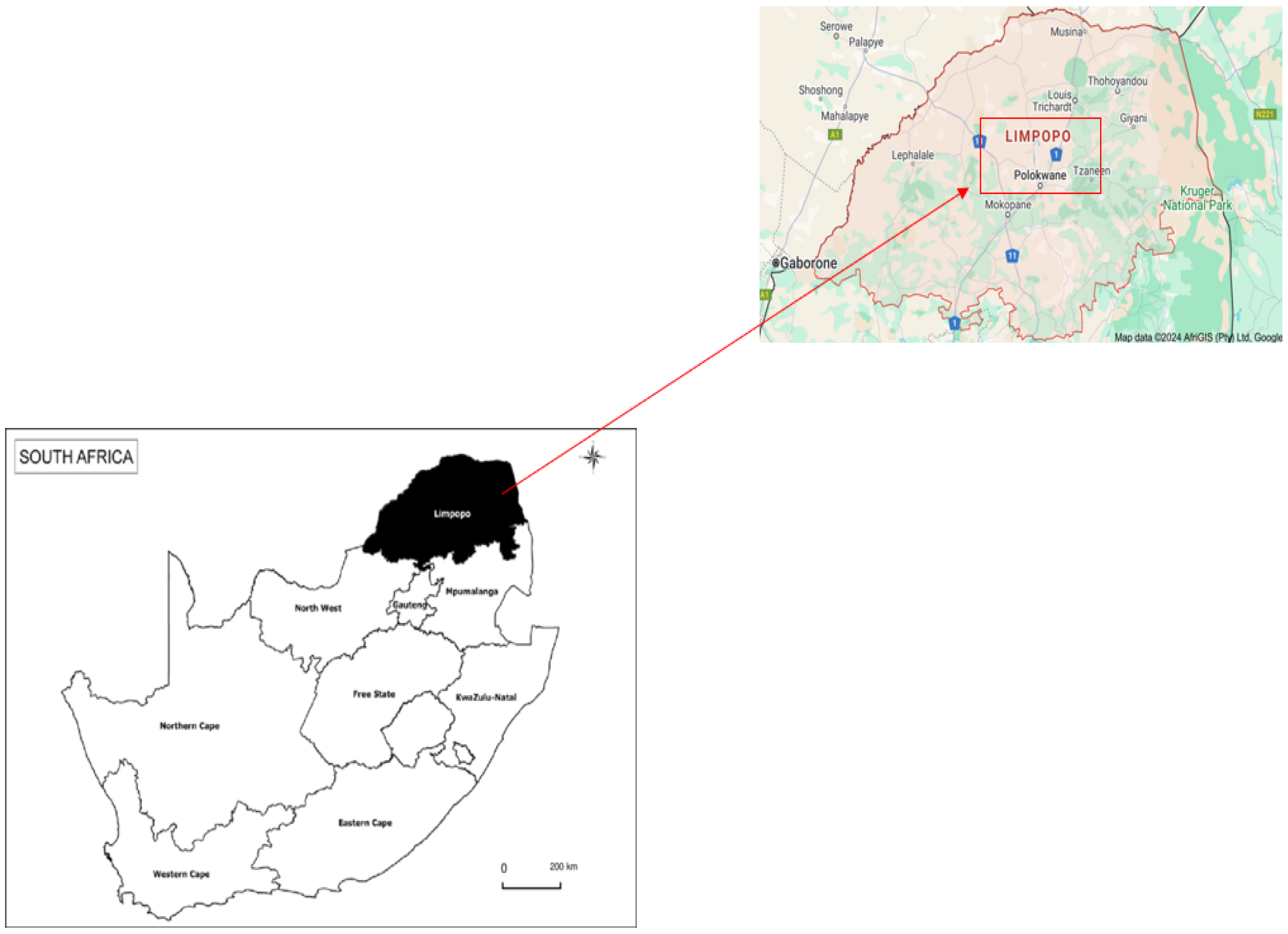
This study uses secondary data sourced from the National Aeronautics and Space Administration (NASA), accessible at https://power.larc.nasa.gov/data-access-viewer/ (accessed on 20 February 2024). The research focuses on Polokwane, also known as Pietersburg, which serves as the capital city of Limpopo Province. Polokwane is geographically positioned at a latitude of 23°54′16.16″ S and a longitude of 29°28′7.86″ E. The dataset encompasses a range of meteorological variables, including surface pressure, wind direction, humidity, and surface temperature. This comprehensive dataset spans from 1 January 2016 to 31 December 2023, with all variables systematically recorded daily at midnight. Figure 1 shows the location of Limpopo Province, extracting Polokwane, the study area. This focus on Polokwane is critical for understanding localised meteorological patterns, which are essential for enhancing the accuracy of wind speed predictions and their applications in renewable energy and environmental planning.

Figure 1.
Geographic location of Polokwane within Limpopo province. Source: https://w.wiki/B2us, accessed on 5 May 2024.
5.2. Analytical Techniques
5.2.1. Vanilla Long Short-Term Memory (Vanilla LSTM)
The Vanilla LSTM network is a recurrent neural network proposed by Hochreiter and Schmidhuber [45]. The Vanilla LSTM network differs from a traditional RNN by retaining past information, which is often lost in traditional RNNs, making learning long-distance dependent information difficult. The Vanilla LSTM is an upgraded recurrent neural network that tries to address RNNs’ limitations in processing long-term memory.
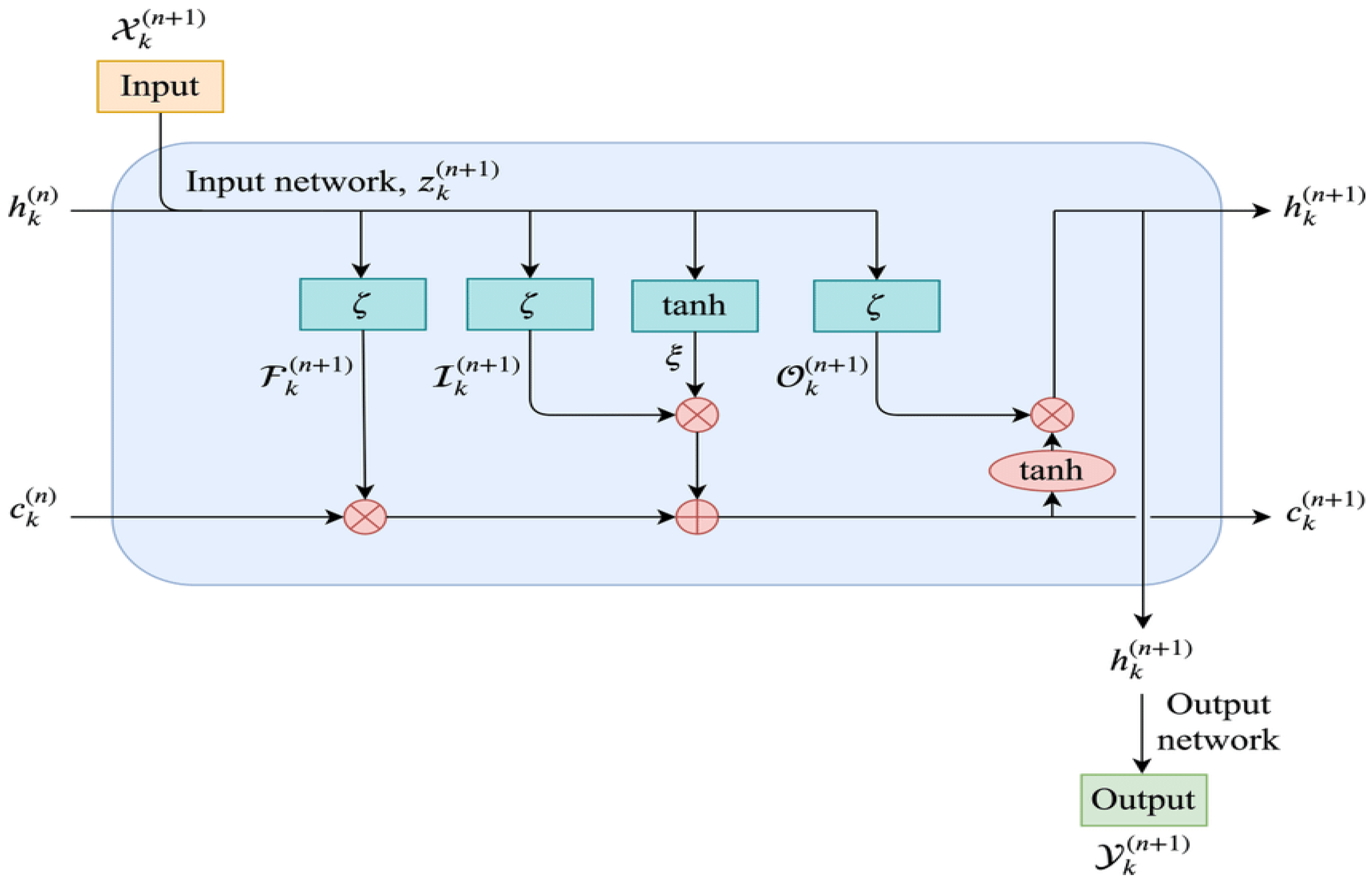
In practical terms, Vanilla LSTM excels in retaining information over extended periods. In time series forecasting, the Vanilla LSTM approach incorporates various gates, significantly enhancing its memory capabilities [45,46]. Let be input values and output values of the existing historical data to be forecasting, then the Vanilla LSTM network can be represented by the following basic system equations,
Figure 2 shows the basic structure of the Vanilla LSTM network as defined by Equations (1)–(5). This visual representation effectively demonstrates the core architecture and operational mechanisms of the Vanilla LSTM model within the context of this study. Figure 2 also highlights the flow of information through the Vanilla LSTM memory cells and gates, showcasing how the network captures and utilises temporal dependencies present in wind speed data.
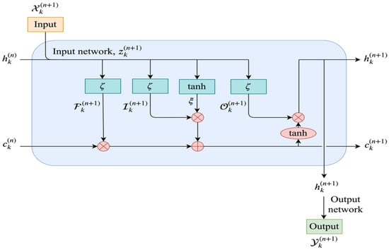
Figure 2.
Basic architecture of the Vanilla LSTM network. Source: https://www.researchgate.net/figure/The-structure-of-LSTM-memory-cell_fig5_342998863, accessed on 30 June 2024.
5.2.2. Convolutional Neural Networks (CNNs)
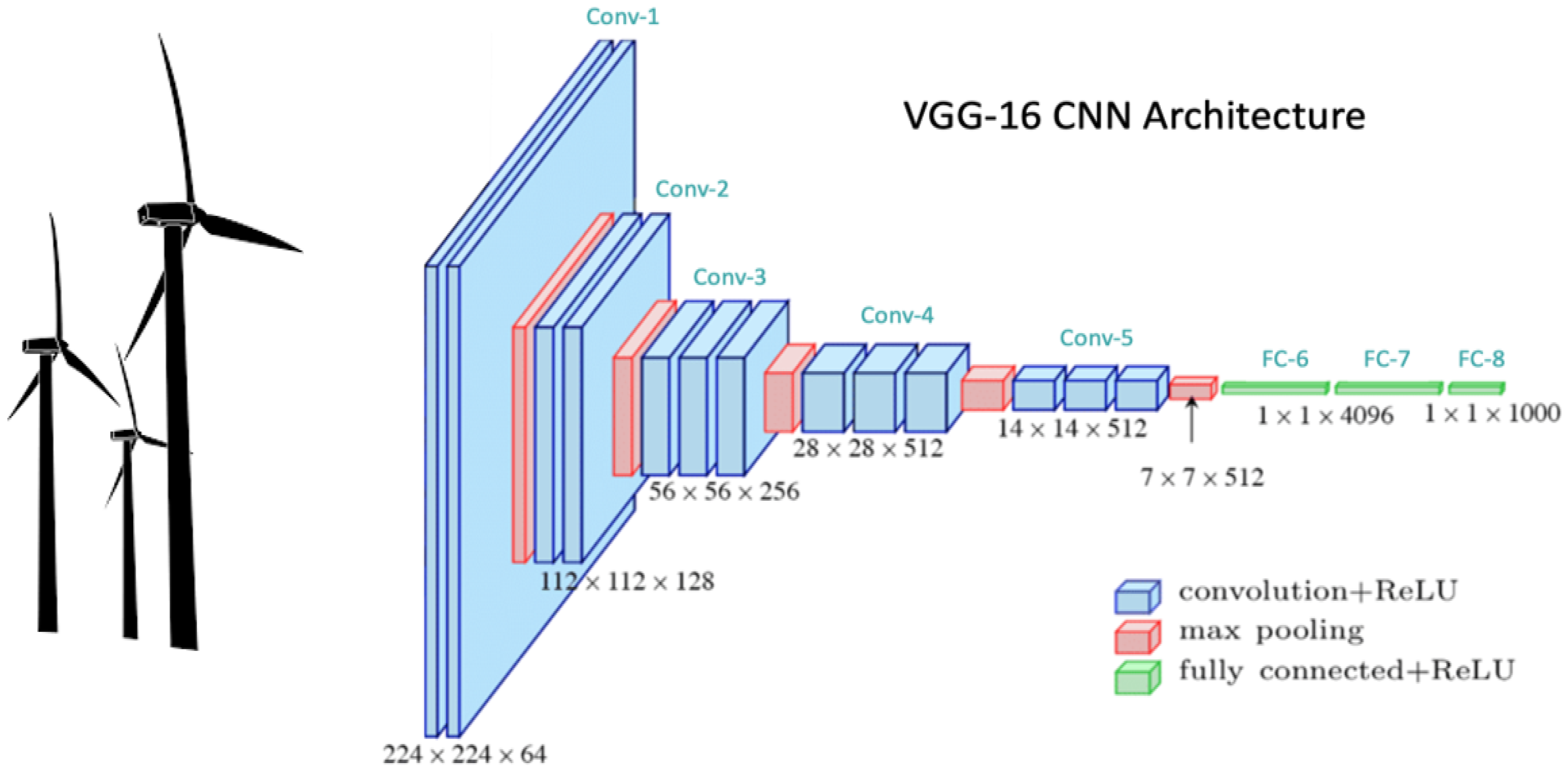
In recent years, deep learning techniques, particularly CNNs, have become a cornerstone for analysing and forecasting complex data patterns, including time series data [47]. CNNs are widely known for their efficacy in spatial data processing, such as image recognition, but their application has been successfully extended to time series forecasting due to their ability to extract critical features from sequential data [48]. This study deploys a CNN to forecast short-term wind speed by leveraging CNNs’ capability to identify intricate patterns in meteorological variables. Through feature extraction and pattern recognition, CNN models offer significant improvements in prediction accuracy compared to traditional forecasting methods. A typical CNN architecture comprises an input, a convolutional, a max pooling, and a fully connected layer, as demonstrated in Figure 3.
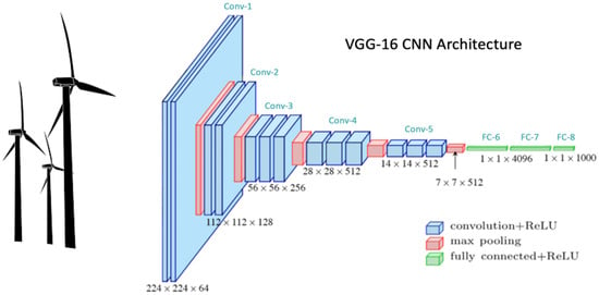
Figure 3.
Basic architecture of a CNN. Source: https://learnopencv.com/wp-content/uploads/2023/01/tensorflow-keras-cnn-vgg-architecture.png, accessed on 18 September 2024.
- Convolution Layer + ReLU Activation
The convolutional layer applies a series of filters (or kernels) to the input data, which, in this case, is the wind speed time series data. These filters slide over the data, performing a dot product with the overlapping portion of the input. After the convolution operation, the output passes through the Rectified Linear Unit (ReLU) activation function. The ReLU function is defined as:
- Max Pooling
This layer reduces the spatial dimensions of the feature maps generated by the convolutional layer, effectively downsampling the data. Max pooling works by selecting the maximum value from a defined window, typically 2 × 2, in the feature map. This operation helps reduce the computational complexity of the model, as well as the risk of overfitting, by concentrating the most important information while discarding irrelevant details.
- Fully Connected Layer + ReLU Activation
Once the data passes through several convolutional and pooling layers, it is flattened into a one-dimensional vector and fed into a fully connected (dense) layer. The fully connected layer aggregates the learned features from the previous layers to make the final predictions. In this layer, each neuron is connected to every neuron in the previous layer, enabling the model to combine features across different parts of the input.
5.2.3. Modelling the r-Largest Order Generalised Extreme Value Distribution ()
The model serves as a method for examining extreme value patterns in statistical analysis. It specifically concentrates on the behaviour of , where it denotes the maximum value within a sequence of independent random variables sharing a common distribution . This model is essential for understanding the statistical behaviour of extreme values, and it can be used to make informed decisions and predict rare future events [8].
The distribution of can be calculated precisely for all the values of m:
The behaviour of as m approaches infinity is examined. However, this analysis is insufficient, as the distribution of will degenerate to a point mass on the upper limit of for each value of z less than . To resolve this issue, a linear re-normalisation of the variable is introduced:
The Gumbel, Fréchet, and Weibull distributions are three popular distributions in EVT. All three distributions have location and scale parameters, and Fréchet and Weibull have an additional shape parameter [49]. Combining these three distributions creates a family of distribution functions with a specific form:
based on the set , with the parameters , , and [8]. This distribution family is referred to as the GEVD and is integral to the methodology of this study. The is an extension of the GEVD, applicable when the data is blocked by different order statistics [13]. When r = 1, the reduces to the standard GEVD, making it a flexible tool for modelling extremes in a variety of contexts.
5.2.4. Parameter Estimation for the
There are various techniques for estimating parameters, such as Bayesian estimation, MLE, and the probability weighted moments (PWM) estimation. In this study, we concentrate on estimating the parameters using MLE. When , the likelihood function is:
and for :
In the context of this study, the optimisation of log-likelihoods yields parameter estimates. These estimated parameters align with those characterising the GEVD for block maxima, but encompass a broader range of extreme observations.
5.2.5. Return Levels
In Equation (9), the allows for the estimation of return levels, denoted as , which correspond to a specific return period for each set of p observations [50]. These return levels provide a critical measure in extreme value analysis, indicating the magnitude of an extreme event expected to be equalled or exceeded once in a given period. The return levels are calculated using the following formula:
5.2.6. Theil–Sen Estimator
In numerous studies on time series analysis, the authors frequently employ the Mann–Kendall test to examine trends and ascertain whether there exists a consistent upward or downward trend over time. Nonetheless, in this study, an alternative methodology known as the Theil–Sen estimator is employed. This approach, pioneered by Sen and Theil [51,52], respectively, entails a median-based slope estimation technique. It presents various advantages over the conventional Mann–Kendall method, being non-parametric and more resilient. The Theil–Sen slope is determined by the following formula:
where a positive value, indicates the existence of a rising trend, while a negative value signifies a declining trend. This method is chosen as the slope estimator for this study due to its robustness, non-parametric nature, and dependable performance in trend estimation.
5.3. Model Evaluation and Validation
5.3.1. Vanilla LSTM Evaluation Metrics
In evaluating the precision of the Vanilla LSTM network, this study uses several metrics, including the mean absolute error (MAE), root mean squared error (RMSE), and mean absolute percentage error (MAPE), to assess the accuracy of predictions. These metrics provide quantitative measures of the model’s performance and enable a comprehensive evaluation of its effectiveness. The mathematical expressions for these metrics are defined as follows:
where signifies the actual values at time t, represents the predicted model values, and n is the sample size of the total observations. These metrics offer comprehensive insights into the accuracy and reliability of our predictive models [53,54]. They enable us to assess how well the models capture the underlying patterns in the data and predict future values, which is crucial for applications in renewable energy and other fields that depend on accurate wind speed forecasting.
5.3.2. Evaluation Metrics for the
In the realm of model evaluation, we turn to the Akaike information criteria (AIC) and Bayesian information criteria (BIC), metrics developed by Akaike and Gideon [55] to gauge the suitability of a model for a specific dataset. The AIC, which has gained prominence in fields such as EVT, machine learning, and econometrics, serves as a guardian against over-fitting proving its effectiveness.
The mathematical expressions defining the AIC and BIC are as follows:
where represents the likelihood of the model, K denotes the total count of model parameters, and N the sample size. The BIC exhibits a preference for simpler models when compared to the AIC. In this narrative of metrics, the AIC and BIC play pivotal roles, guiding researchers towards models that strike a balance between complexity and fit. A better fit is indicated by lower AIC and BIC values.
6. Empirical Findings and Analysis
Table 1 outlines the descriptive statistics for wind speed data collected in Polokwane, South Africa, using an anemometer over the sampling period spanning from 1 January 2016 to 1 December 2023, providing essential insights into the variability and characteristics of wind patterns in the region. Table 1 provides crucial insights into the variability and characteristics of wind patterns in the region. The table includes key statistical measures such as the minimum, median, mean, maximum, skewness, kurtosis, and standard deviation of the wind speeds. Figure 4 presents the seasonal wind speed trend analysis for 2023.

Table 1.
Descriptive statistics of the wind speed data used in this study.
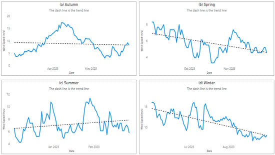
Figure 4.
Seasonal wind speed trend analysis for 2023.
A positive skewness value of 0.68 indicates that the distribution is skewed to the right, meaning there are fewer lower wind speeds and more higher wind speeds. The distribution of the sampled data is leptokurtic, meaning it has heavier tails and a more peaked shape compared to a normal distribution, with a kurtosis value of 4.01. The standard deviation of wind speeds, representing the amount of variation or dispersion of wind speeds around the mean, was 2.86 m/s. This indicates how much individual wind speed measurements deviate from the average wind speed.
In terms of wind turbine performance for electricity generation across the seasons, Table 2 reveals distinctive patterns in each season. Summer exhibits moderate wind conditions, with a median wind speed of 7.34 m/s, indicating a reasonably efficient period for wind power generation. Winter stands out as the most wind efficient season with a higher median wind speed of 7.96 m/s, although it also presents the potential for extreme wind events, as indicated by a positively skewed distribution and higher kurtosis. Autumn showcased a favourable median wind speed of 8.90 m/s, offering another promising season for wind power generation, while its distribution remains relatively stable. These findings underscore the seasonal dynamics of wind energy potential, highlighting the need for tailored strategies to optimise electricity generation throughout the year.

Table 2.
Descriptive statistics per season.
6.1. Seasonal Wind Speed Trends for 2023
Figure 4 provides the seasonal wind speed trend analysis for the four seasons of 2023, namely autumn, spring, summer and winter. In autumn, the wind speed trend is slightly downward while there is a clear downward wind speed trend in spring and winter. On the contrary, summer has an upward wind speed trend.
6.2. Test for Stationarity
- Augmented Dickey–Fuller (ADF)
Before presenting the ADF test results, it is pertinent to introduce its application in assessing the stationarity of wind speed data in our focus area. The ADF test serves as an important test in determining whether the observed wind speed series exhibits a stationary behaviour, a crucial consideration for a range of analytical applications.
The hypotheses for the ADF test are as follows:
:
The time series data has a unit root (i.e., it is non-stationary).
:
The time series data does not have a unit root (i.e., it is stationary).
The results of the ADF test revealed that the wind speed in Polokwane is stationary (), indicating the data is suitable for time series modelling and further analysis.
6.3. Theil–Sen Non-Parametric Trend Plot
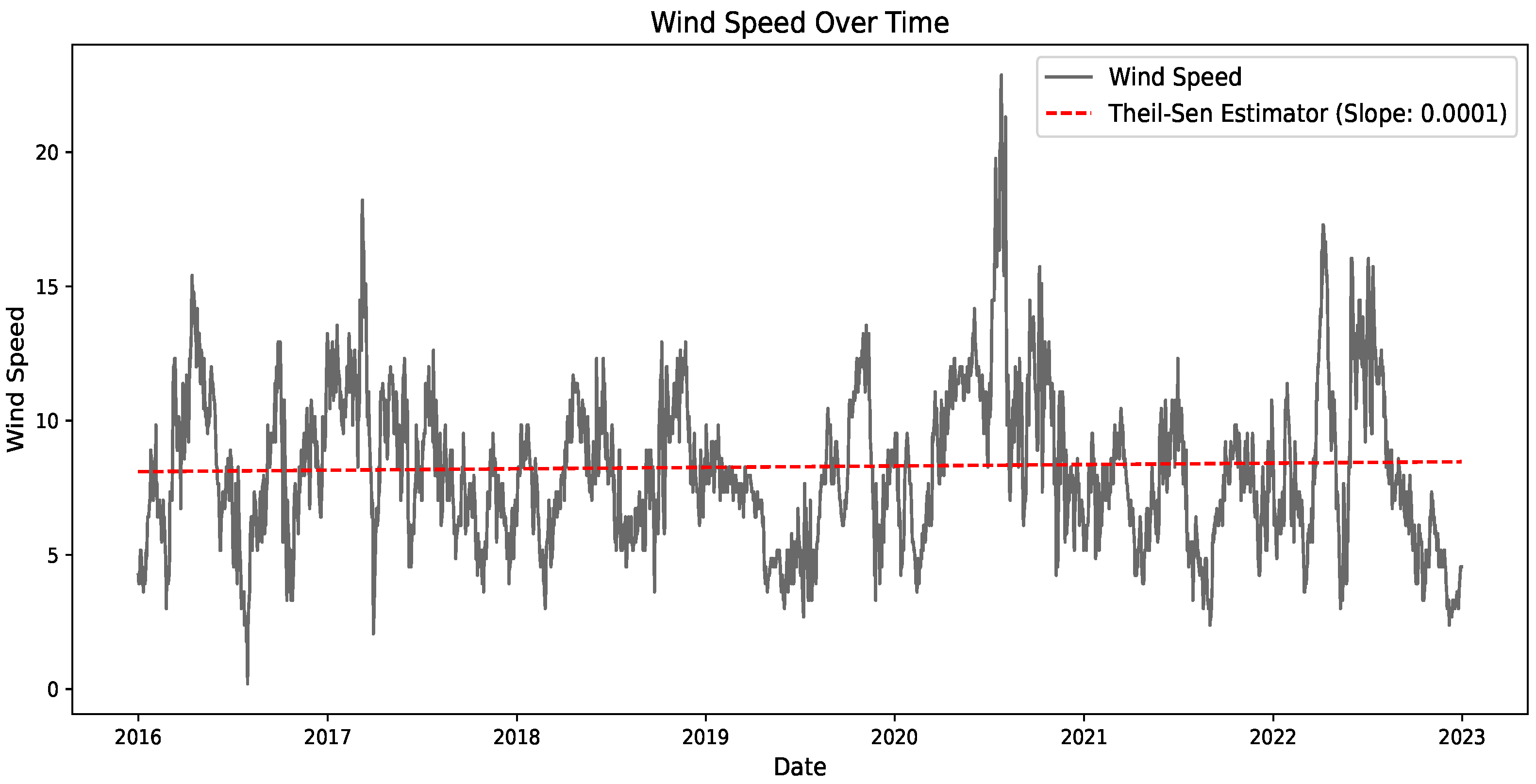
Figure 5 presents the outcomes of the Theil–Sen estimator within the framework of our focused geographical area. The Theil–Sen estimator value of −0.0002 indicates the potential linear relationship between the two variables, wind speed and date/time. The negative test statistic of −3.4644 suggests that the estimated slope differs from zero, indicating a potential negative association between the two variables. With a degree of freedom 2555, this statistical analysis captures the variability in the data. In the context of wind power generation, this slightly negative slope could imply a slight reduction in wind power output or efficiency as wind speed increases, though the magnitude of this effect is minimal (−0.0002).
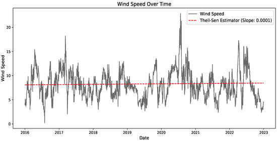
Figure 5.
Trend slope plot.
6.4. Machine Learning
6.4.1. Vanilla LSTM and CNN Results
This section presents the findings obtained through utilising the Vanilla LSTM and CNN models. The model forecasting accuracy was assessed using the traditional metrics such as MAE, RMSE, and MAPE. Furthermore, predictions for the next five years (2024–2028) along with 95% confidence intervals are included. The following are the prediction results for both the training and testing sets after fitting to the Vanilla LSTM and CNN models.
Figure 6 illustrates the performance of the Vanilla LSTM and CNN models in predicting wind speed. The blue line represents the actual wind speed, while the green and orange lines denote the Vanilla LSTM and CNN predictions, respectively. Both models were trained on historical wind speed data and tested on previously unseen data to evaluate their performance. The close alignment between the actual values and the model predictions indicates that both models perform well, with minimal prediction error. This strong correlation highlights the ability of the models to accurately capture the underlying patterns in wind speed data, proving their reliability for forecasting purposes. The high accuracy and low error rates suggest that these models can be valuable tools for various applications, such as renewable energy management, where accurate wind speed forecasting is crucial.
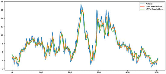
Figure 6.
Training and testing predictions of Vanilla LSTM and CNN models.
Figure 7 and Table 3 provide a comprehensive evaluation of the performance of both the Vanilla LSTM and CNN models on the testing set using various metrics such as MAE, RMSE, MAPE, and model accuracy. The metrics illustrate a strong alignment between predicted and actual wind speed values, demonstrating the robustness and precision of both models in forecasting. Specifically, the CNN model performed slightly better, achieving a monthly MAE of 0.53, compared to the 0.70 of the Vanilla LSTM model, with a corresponding RMSE of 0.75 for CNN versus 0.94 for Vanilla LSTM, indicating lower overall error in the CNN model. Similarly, the CNN’s MAPE values of 0.09 further highlight its minimal deviation from actual values, as opposed to 0.27 for the Vanilla LSTM. Accuracy-wise, CNN outperformed LSTM, with 88.66% for the monthly-time-step model, compared to Vanilla LSTM’s 85.56%.

Figure 7.
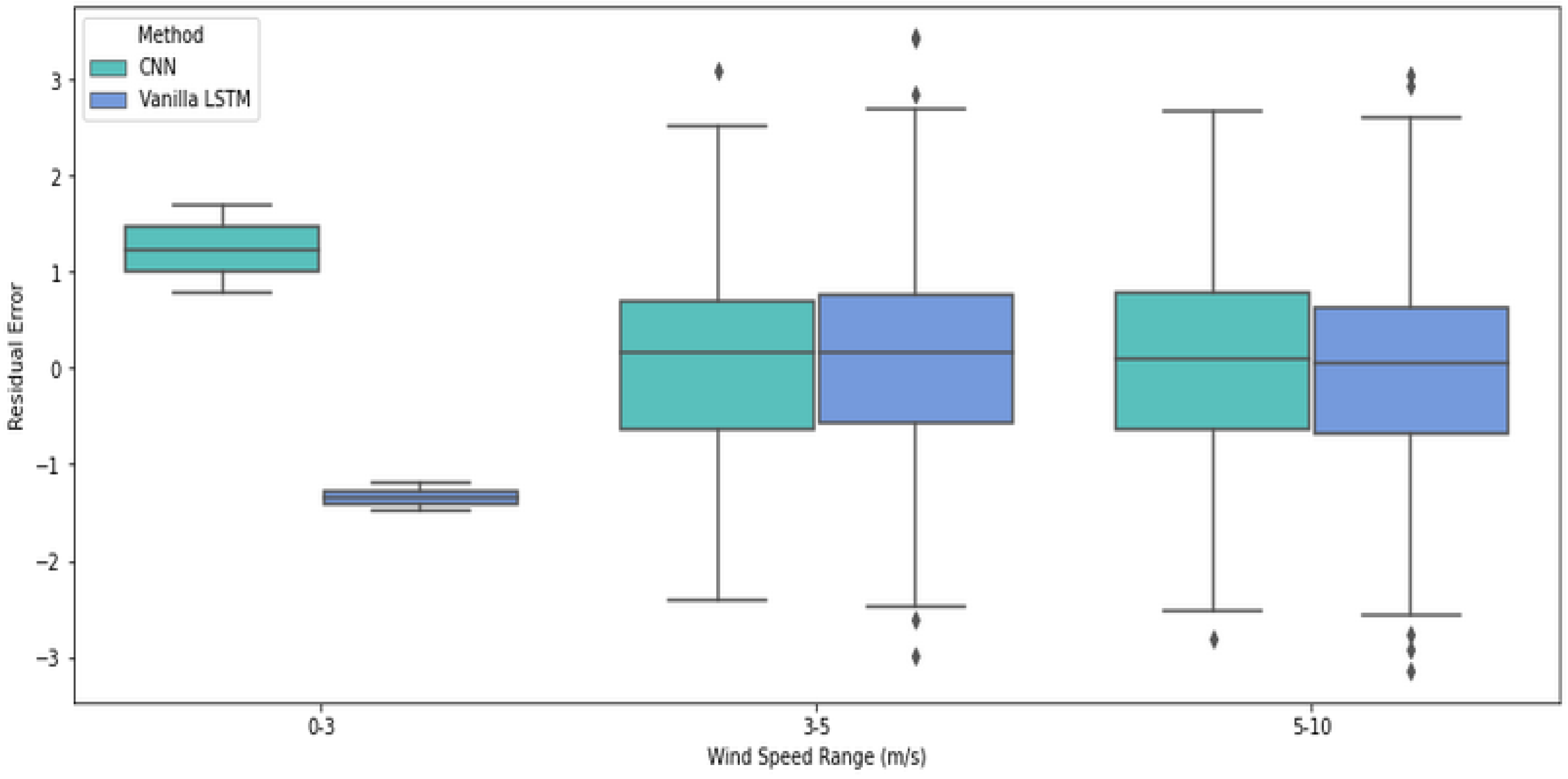
Boxplot of the residual errors of each method with different ranges of the wind speed.

Table 3.
Performance summary for all models executed according to time steps.
The boxplots of residual errors (Figure 7) further demonstrate the comparative performance across different wind speed ranges. In the low wind speed range (0–3 m/s), both models exhibit minimal residual errors, with CNN having a slight advantage. In higher ranges (3–5 m/s and 5–10 m/s), the CNN model again shows more consistency, with smaller variations in residual error, underscoring its superior performance in handling higher wind speeds.
These findings affirm the applicability of both models in real-world wind speed forecasting scenarios, with CNN offering a marginally better overall performance. The results suggest that these models can be effectively used for future predictions, potentially leading to more accurate and reliable wind speed forecasts, particularly for renewable energy management. This not only establishes a solid foundation for the use of both Vanilla LSTM and CNN models in forecasting endeavours but also paves the way for further advancements in predictive analytics and time series forecasting.
6.4.2. Training and Validation Loss between Vanilla LSTM and CNN Models
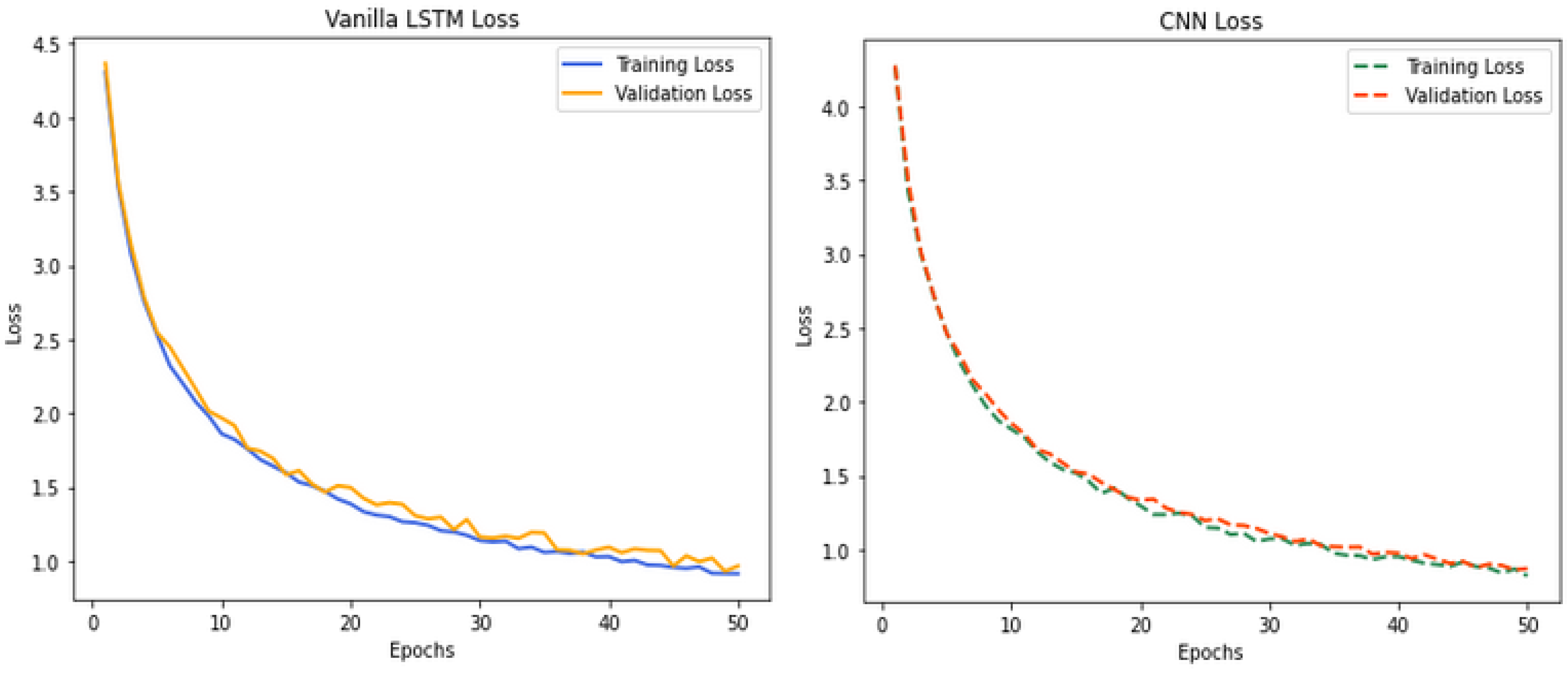
Figure 8 presents a comparison of the training and validation loss for the Vanilla LSTM and CNN models across 50 epochs. The left subplot depicts the Vanilla LSTM model, where both training and validation loss exhibit a steady decline throughout the epochs. The gap between the training and validation loss is minimal, suggesting that the model generalises well without significant overfitting. However, a slight plateau is observed towards the latter epochs, indicating diminishing improvements in the loss reduction.
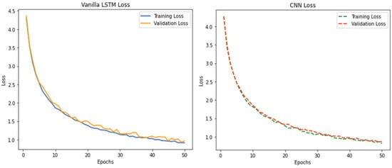
Figure 8.
Training and validation loss of Vanilla LSTM and CNN models.
The right subplot illustrates the CNN model performance, which similarly shows a consistent reduction in both training and validation loss. However, the CNN model demonstrates slightly superior performance in terms of both lower training and validation losses compared to the Vanilla LSTM. The losses are closely aligned, indicating robust generalisation and effective training.
Overall, both models show effective learning over time, though the CNN appears to converge slightly faster and achieves marginally better loss metrics. This suggests that the CNN model may provide more accurate predictions within 50 epochs, making it a more efficient model for forecasting wind speed in Polokwane, South Africa.
6.5. Model Performance Comparison: Vanilla LSTM and CNN Wind Speed Forecasts
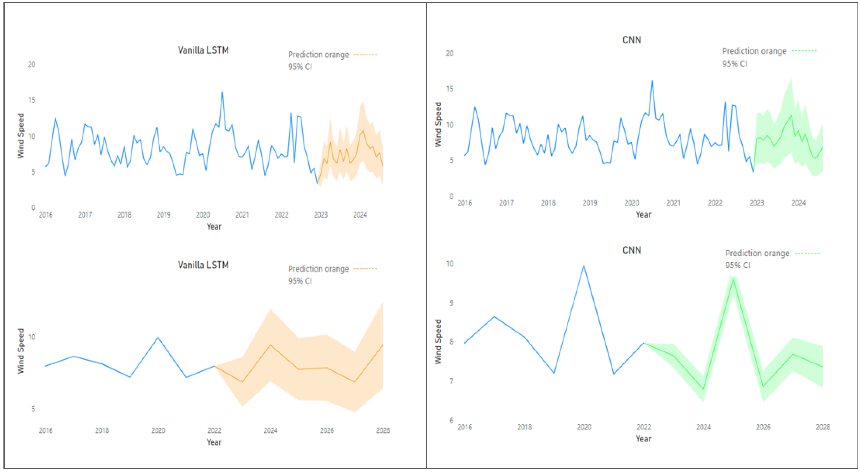
Figure 9 presents a comparison between the forecasting performance of Vanilla LSTM and CNN models for predicting wind speed. The findings suggest that the CNN model outperforms Vanilla LSTM in terms of stability and reliability. The Vanilla LSTM predictions align well with historical wind speed trends, indicating a moderate ability to generalise daily and yearly patterns; however, its wider confidence interval (CI), particularly from 2024 onwards, reflects higher uncertainty in long-term forecasts. This broader CI suggests that the Vanilla LSTM model may be overfitting certain patterns or anomalies in the data, resulting in more pronounced fluctuations in its predictions for 2025–2028. By comparison, the CNN model demonstrates a narrower, green-shaded CI, implying a lower degree of uncertainty in its forecasts. The CNN yearly average predictions remain consistent and stable, with limited fluctuations, as evidenced by the narrow confidence bounds extending from 2023 to 2028. This suggests the CNN model is more reliable for long-term forecasting, as it maintains smoother predictions and exhibits greater confidence in future wind speed trends. The gradual increase in predicted wind speeds, coupled with the narrower CI, highlights the model’s capacity for stable and confident forecasting over an extended period.
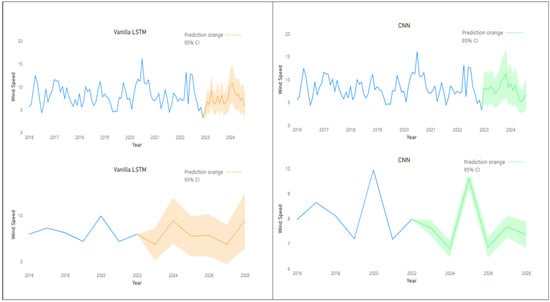
Figure 9.
(Top left panel): Vanilla LSTM daily wind speed predictions; (Top right panel): CNN daily wind speed predictions; (Bottom left panel): Vanilla LSTM yearly wind speed predictions; (Bottom right panel): CNN yearly wind speed predictions.
Overall, while Vanilla LSTM proves effective in capturing variability and following historical data, its higher uncertainty makes it less dependable for long-term forecasting. Meanwhile, the CNN model provides a more robust and confident forecast, making it a more suitable choice for reliable, long-term wind speed predictions. The comparison underscores the value of the CNN model in offering tighter confidence bounds and more consistent performance, particularly when precision in extended forecasts is essential. Therefore, this study recommend that the government incorporate these forecasts into long-term energy and infrastructure planning, using the CNN model for reliable projections. Investing in renewable energy, particularly wind farms, based on these forecasts, could not only boost energy independence but also contribute to South Africa climate action goals.
6.6. Short-Term Vanilla LSTM and CNN Predictions
Table 4 presents the predicted average wind speeds for the years 2024 to 2028 using the Vanilla LSTM and CNN models. The forecasts indicate a fluctuating trend in wind speeds over the five-year period, with a notable decline in 2027 and a recovery in 2028. These findings suggest that Polokwane will experience moderate wind speed events, with some variability across the forecasted years. A 95% confidence interval (CI) is included to account for uncertainty, providing both lower and upper bounds for each prediction. The upper bound for 2028 is particularly high, suggesting the possibility of extreme wind speed events in that year. When comparing the two models based on the confidence intervals, the CNN model exhibits narrower intervals in most years, particularly in 2025 and 2026, where the range of possible outcomes is smaller. This suggests that the CNN model provides more precise predictions and may be considered more reliable for forecasting wind speeds during this period. Conversely, the Vanilla LSTM model tends to have wider intervals, indicating greater uncertainty in its predictions.

Table 4.
Predicted average wind speed for the next five years.
These predictions demonstrate the value of both models in forecasting wind speed trends. The CNN model, with its tighter confidence intervals, may offer better precision, while the Vanilla LSTM captures broader potential variations. The ability of these models to accommodate uncertainty and predict trends allows for better preparation and planning, particularly for extreme weather events. The inclusion of confidence intervals further strengthens the robustness of the predictions, supporting more informed decision-making in managing wind-related risks.
6.7. Extreme Value Theory (EVT)
Fitting the r-Largest Order Statistics
This section presents the findings obtained from applying the r-largest order to the dataset. The r-largest order statistics ranged from 1 to 5. Each order was subsequently fitted to the to estimate the location, scale, and shape parameters. The analysis aimed to determine the optimal r-order statistic. The parameters were estimated using the MLE method. The standard deviation for each parameter was computed, and the results are presented in Table 5.

Table 5.
optimal order assessment.
Table 4 summarises the optimal order results with r-order sizes ranging from 1 to 5, denoted by r. These insights shed light on the statistical traits of extreme events, crucial for their comprehension and modelling. The estimated location parameter () gradually decreased after r = 2 increased, indicating a shift towards lower central tendencies in extreme event data. Standard errors decreased with increasing r, enhancing confidence in location parameter estimates for larger order.
The scale parameter () also gradually decreased after the second order. For instance, ranged from 2.526 to 2.496 across the r-order sizes. Conversely, the shape parameter () became less negative after the second order, indicating a shift towards heavier-tailed distributions for larger r values. These findings are vital for understanding extreme events and tail behaviour, assisting in the selection of optimal r-order size for prediction and risk assessment.
6.8. Goodness of Fit
Table 6 shows that increasing the order statistics from second order leads to higher negative log-likelihood, AIC, and BIC values as r increases from size two to five, indicating poorer fits to the data. Striking a good balance between model goodness of fit and complexity is crucial for selecting the optimal r. In this context, emerges as the preferred fit, offering significantly lower AIC and BIC values compared to other models, while maintaining a lower negative log-likelihood. Thus, choosing r = 2 effectively balances data explanation and complexity, making it the most favourable choice among the options.

Table 6.
Goodness of fit evaluation metrics for optimal order selection.
6.9. Diagnostic Plots for
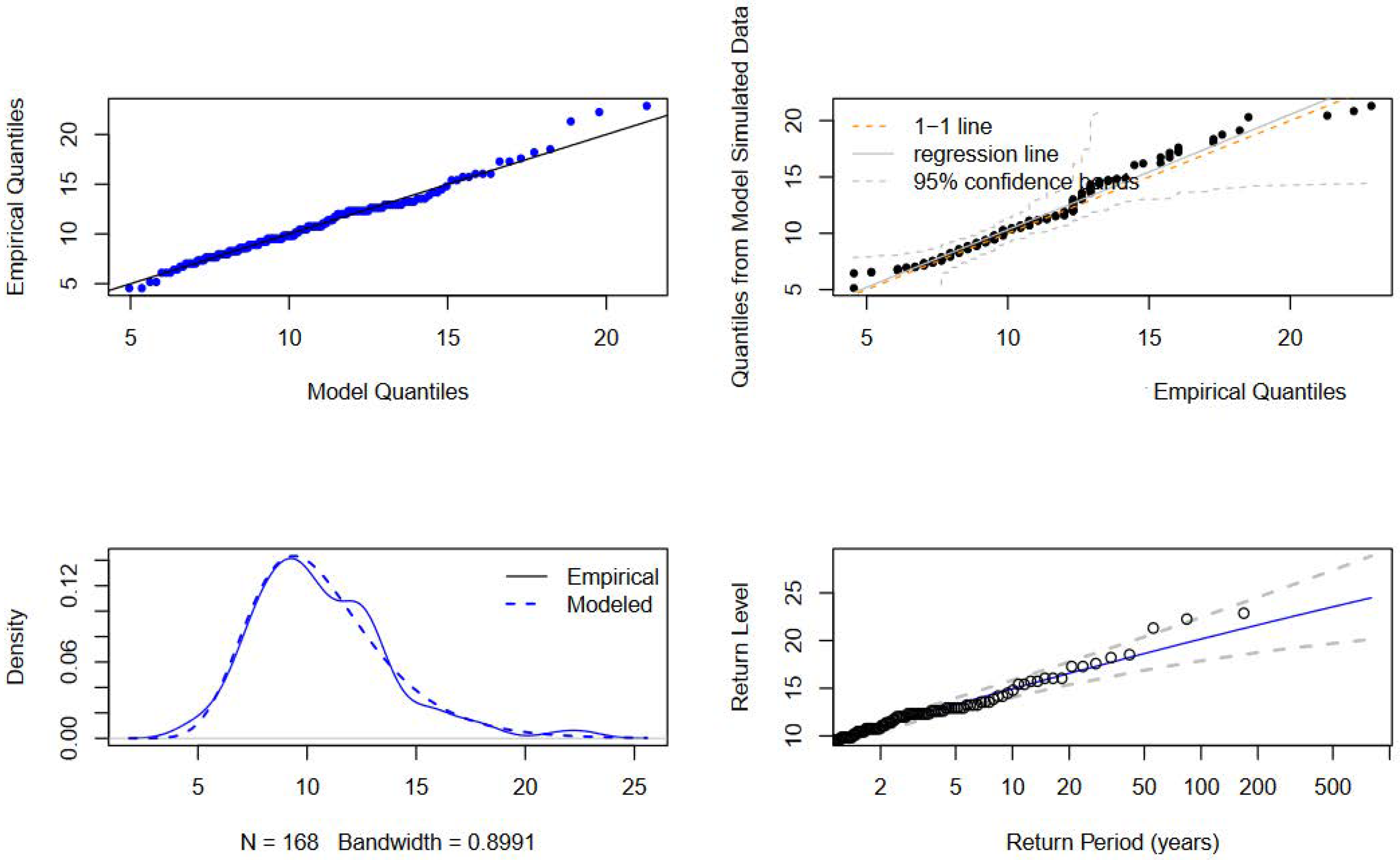
Another method for determining the optimal order size involves a comprehensive approach that combines visual inspection of the data using graphical diagnostic plots with insights derived from the results presented in Table 6. This approach particularly emphasises selecting the model with the smallest AIC and BIC values. Figure 10 presents the diagnostic plots for . These plots provide a visual assessment of the model fit, showcasing empirical quantiles against model quantiles, quantiles from model-simulated data against empirical quantiles, the density of empirical versus modelled data, and return levels for various return periods. These visual tools are crucial for evaluating the model performance and ensuring the robustness of the parameter estimates. By leveraging both statistical and graphical diagnostics, we aim to refine our model selection process, enhancing the accuracy and reliability of our extreme value predictions.
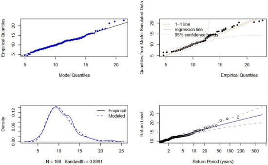
Figure 10.
diagnostic plots.
Figure 10 provides compelling evidence supporting the suitability of the model for describing wind speed behaviour. This is clearly demonstrated by the strong alignment observed in both the P–P and Q–Q plots, indicating a close fit between the model’s predicted values and the empirical data. Additionally, the return level plot shows a clear increasing trend, further confirming the model’s effectiveness in capturing the behaviour of extreme wind events. Moreover, the density plot illustrates a close match between the fitted density curve and the empirical density distribution, highlighting the robust agreement between the model and the actual data. This consistency underscores the reliability of the model in accurately representing wind speed characteristics.
The findings in Table 6 and Figure 10 suggest that the model has the potential to significantly enhance our understanding and prediction of extreme wind events, which is crucial for effective wind power generation strategies. This is particularly crucial for the development of resilient and efficient wind energy systems, as it provides a reliable framework for analysing and forecasting extreme weather conditions.
6.10. Return Levels for
Table 7 provides valuable insights into return levels across different return periods, ranging from 5 to 300 years. These levels act as significant indicators in the distribution, offering predictions regarding the severity of extreme events over specific time frames. For instance, the 5-year return level is recorded at 13.03 m/s, suggesting an event of this magnitude is anticipated approximately every 5 years. This indicates a relatively low probability of , suggesting a 20% chance of extreme wind speed event occurring in the next 5 years compared to the maximum rare event observed during 2016 to 2023. The 100-year return level estimate is 20.14 m/s, which is lower than the maximum observed wind speed of 22.86 m/s for the period 2016 to 2023.

Table 7.
Return levels.
The 250-year return level, standing at 22.10 m/s, represents an exceedingly rare event expected approximately once every 250 years. This event is closely comparable to the maximum event observed in the past decade. Furthermore, the 300-year return level, indicating an event occurring once every three centuries, underscores an exceptionally rare event with a very low probability of a 0.3% chance of the rare extreme wind event occurring. Compared to the highest recorded wind speed of 22.86 m/s in Table 1, the 300-year return level denotes a higher magnitude event. Therefore, the 300-year return level becomes a crucial measure for assessing the potential risks associated with encountering extremely severe wind events in the Polokwane region. It is worth noting that such rare events have a high probability of occurrence during the winter and autumn seasons, as highlighted in Table 2, with high maximum wind speed magnitudes present in the seasonal summary statistics.
Combining the results from Table 4 and Table 7, it is evident that both the Vanilla LSTM and CNN models provide comparable predictions for the average wind speed in Polokwane over the next five years. Specifically, in 2028, the average wind speed is projected to be 9.43 m/s with confidence bounds of 6.82 and 13.44 according to the Vanilla LSTM model. Similarly, the CNN model predicts a slightly higher average wind speed of 9.59 m/s, with confidence bounds of 7.63 and 12.11. This overlap in their respective confidence intervals indicates that both models are effective in capturing wind speed variability, thereby supporting the robustness of these deep learning approaches in forecasting wind dynamics. Moreover, the model, which focuses on predicting extreme wind events, forecasts a return level of 13.03 m/s for a 5-year return period, and 22.89 m/s for a 300-year return period. This extreme value prediction of 13.03 m/s for the 5-year period aligns well within the confidence bounds provided by the Vanilla LSTM and CNN models for the year 2028, thereby reinforcing the consistency and reliability of the three models under different forecasting conditions. The consistency observed between these models suggests that a hybrid modelling approach may be beneficial. Specifically, incorporating the Vanilla LSTM and CNN models for short-term average wind speed forecasting, alongside the GEVD model for extreme event prediction, would provide a more comprehensive view of the wind climate in Polokwane. This combination would allow for enhanced decision-making in the design and implementation of wind energy systems, ensuring that both typical and extreme wind conditions.
7. Conclusions and Recommendation
This study conducted an in-depth analysis of wind speed forecasting in Polokwane, shedding light on statistical properties, seasonal variations, and future predictions. The primary aim was to forecast short-term wind speed events using Vanilla LSTM and CNN and long-term wind speed events using the . Historical data from Polokwane suggests a low likelihood of extreme wind events. Seasonal analysis revealed that winter and autumn are the most efficient seasons for wind power generation and also indicate the potential for extreme wind events. The ADF test confirmed that the time series data is stationary, suggesting a constant mean and variance over time, which is essential for accurate modelling and forecasting.
The CNN network model demonstrated accurate wind speed forecasts with low error rates and high predictive accuracy, supported by low evaluation metrics such as MAE, RMSE, and MAPE. Given the robustness of both Vanilla LSTM and CNN in forecasting average wind speeds and the ability of the GEVD model to capture extreme wind events, it is recommended to adopt a hybrid forecasting strategy that leverages the strengths of all three models. This approach would enable practitioners to more effectively plan for both regular and extreme wind scenarios, thereby improving the resilience and efficiency of wind energy systems. Furthermore, the minor overestimation of wind speeds by the Vanilla LSTM and CNN models warrants a continuous model refinement strategy and an evaluation against real-world data to enhance predictive accuracy. Overall, by integrating the predictive strengths of deep learning with the extreme event analysis of the GEVD model, it is possible to develop a more resilient wind energy strategy tailored to the local wind climate.
In conclusion, this study lays a robust foundation for wind power generation, offering valuable insights for stakeholders in renewable energy and environmental planning. These findings contribute to more sustainable and informed decision-making in Limpopo province. This study offers a set of recommendations in the domain of energy management and sustainability. The following recommendations are proposed for future research direction:
- Employ advanced machine learning techniques, such as Kolmogorov–Arnold networks (KANs) and temporal convolutional networks (TCNs). These methods can capture complex relationships within meteorological variables and geographical features, thereby enhancing the accuracy and efficiency of wind forecasting.
- Investigate the use of modern EVT techniques, such as blended GEVD (bGEVD) and generalised autoregressive conditional heteroskedasticity-GEVD (GARCH-GEVD), to present a refined approach to analysing extreme events in wind speed data. By incorporating bGEVD and GARCH-GEVD, future research can gain a deeper understanding of the tail behaviour of wind speed distributions, thereby improving the assessment of potential risks associated with extreme wind events.
- Expand the geographical scope to encompass all nine provinces of South Africa for a clear understanding of regional wind patterns. A broader geographical scope will enable the research to capture diverse wind patterns, ensuring a more robust and representative analysis.
- Encourage collaboration and knowledge sharing among research institutions, government entities, and industry stakeholders. By encouraging collaboration among research institutions, government entities, and industry stakeholders, research outcomes and data can be leveraged collectively. The exchange of knowledge and data can facilitate a more comprehensive understanding of the challenges and opportunities in wind power generation.
8. Limitations
Wind is a magnificent, boundless, and cost-free clean source of renewable energy for electricity generation. At the same time, it is essential to recognise specific constraints within wind power generation. This study focused on Polokwane, the capital city of Limpopo province, limiting the geographical scope to a semi-developed urban area with specific meteorological conditions. This geographical focus presents a limitation, as addressing the issue of load-shedding requires a broader perspective encompassing all cities across South Africa. Additionally, there is not much existing research globally, especially in South Africa, that combines machine learning and EVT to forecast wind speed. This lack of literature makes it difficult to compare and contextualise the findings of this study.
Another limitation is the availability and quality of wind speed data in South Africa. This presents a constraint on the generalisability of the findings, as a more comprehensive dataset spanning several decades would provide a stronger foundation for EVT-based models to accurately capture extreme occurrences and establish more robust patterns. Without such extensive data, the ability to draw conclusive insights on wind behaviour and its long-term trends is limited, which could affect the reliability of the predictions. Despite these limitations, the study provides a foundational approach to combining machine learning and EVT for wind speed forecasting in a South African context, highlighting the potential for enhancing wind power generation and addressing the energy challenges faced by the region.
Author Contributions
Conceptualisation, K.M. and D.M.; methodology, D.M.; software, K.M.; validation, K.M. and D.M.; formal analysis, K.M. and D.M.; investigation, K.M. and D.M.; resources, K.M. and D.M.; data curation, K.M.; writing—original draft preparation, K.M. and D.M.; writing—review and editing, K.M. and D.M.; visualisation, K.M. and D.M.; supervision, D.M.; project administration, K.M. and D.M.; funding acquisition, D.M. All authors have read and agreed to the published version of the manuscript.
Funding
There authors received no funding for carrying out this research.
Informed Consent Statement
Not applicable since the study does not involve humans.
Data Availability Statement
The dataset was obtained from NASA, focus area Polokwane in Limpopo province. Data are from 1 January 2016 to 31 December 2023, and all features are recorded daily at Midnight (00:00). The data can be accessed at https://power.larc.nasa.gov/data-access-viewer/, accessed on 5 May 2024.
Acknowledgments
The authors would like to thank the National e-Science Postgraduate Teaching and Training Platform (NEPTTP) and the University of Limpopo for funding the article processing charges and to the numerous reviewers for their valuable comments.
Conflicts of Interest
The authors declare no conflicts of interest. The funders had no role in the design of the study, in the writing of the manuscript, or in the decision to publish the results.
References
- Zhang, J.; Lu, J.; Pan, J.; Tan, Y.; Cheng, X.; Li, Y. Implications of the development and evolution of global wind power industry for china—An empirical analysis is based on public policy. Energy Rep. 2022, 8, 205–219. [Google Scholar] [CrossRef]
- Golshani, A.; Sun, W.; Sun, K. Real-time optimized load recovery considering frequency constraints. IEEE Trans. Power Syst. 2019, 34, 204–4215. [Google Scholar] [CrossRef]
- Ahmed, K.M.; Khan, M.A.; Siddiqui, I.; Khan, S.; Shoaib, M.; Zia, I. Wind speed prediction from site meteorological data using artificial neural network. In Proceedings of the 2022 Global Conference on Wireless and Optical Technologies (GCWOT), Malaga, Spain, 14–17 February 2022; pp. 1–8. [Google Scholar]
- Antonini, E.G.; Caldeira, K. Atmospheric pressure gradients and Coriolis forces provide geophysical limits to power density of large wind farms. Appl. Energy 2022, 14, 116048. [Google Scholar] [CrossRef]
- Fischereit, J.; Brown, R.; Larsén, X.G.; Badger, J.; Hawkes, G. Review of mesoscale wind-farm parametrizations and their applications. Bound.-Layer Meteorol. 2022, 182, 175–224. [Google Scholar] [CrossRef]
- Jensen, J.P.; Skelton, K. Wind turbine blade recycling: Experiences, challenges and possibilities in a circular economy. Renew. Sustain. Energy Rev. 2018, 97, 165–176. [Google Scholar] [CrossRef]
- Wang, Z.; Hong, T.; Piette, M.A. Building thermal load prediction through shallow machine learning and deep learning. Appl. Energy 2020, 263, 11–46. [Google Scholar] [CrossRef]
- Coles, S.; Bawa, J.; Trenner, L.; Dorazio, P. An Introduction to Statistical Modelling of Extreme Values; Springer: London, UK, 2020; Volume 208, p. 208. [Google Scholar]
- Singirankabo, E.; Iyamuremye, E.; Habineza, A.; Nelson, Y. Statistical modelling of maximum temperature in Rwanda using extreme value analysis. Open J. Math. Sci. 2023, 7, 180–195. [Google Scholar] [CrossRef]
- Salehin, I.; Talha, I.M.; Hasan, M.M.; Dip, S.T.; Saifuzzaman, M.; Moon, N.N. An artificial intelligence based rainfall prediction using LSTM and neural network. In Proceedings of the 2020 IEEE International Women in Engineering (WIE) Conference on Electrical and Computer Engineering (WIECON-ECE), Bhubaneswar, India, 26–27 December 2020; pp. 5–8. [Google Scholar]
- Melina, S.; Napitupulu, H.; Mohamed, N. A conceptual model of investment-risk prediction in the stock market using extreme value theory with machine learning: A semisystematic literature review. Risks 2023, 11, 60. [Google Scholar] [CrossRef]
- Simas, M.; Pacca, S. Socio-economic benefits of wind power in Brazil. J. Sustain. Dev. Energy Water Environ. Syst. 2020, 263, 27–40. [Google Scholar] [CrossRef][Green Version]
- Metwane, M.K.; Maposa, D. Extreme Value Theory Modelling of the Behaviour of Johannesburg Stock Exchange Financial Market Data. Int. J. Financ. Stud. 2023, 11, 130. [Google Scholar] [CrossRef]
- Elsaraiti, M.; Merabet, A. A comparative analysis of the arima and lstm predictive models and their effectiveness for predicting wind speed. Energies 2021, 14, 6782. [Google Scholar] [CrossRef]
- Murugesan, R.; Mishra, E.; Krishnan, A.H. Deep learning based models: Basic LSTM, Bi LSTM, Stacked LSTM, CNN LSTM and Conv LSTM to forecast Agricultural commodities prices. Res. Sq. 2021. [Google Scholar] [CrossRef]
- Mutavhatsindi, T.; Sigauke, C.; Mbuvha, R. Forecasting hourly global horizontal solar irradiance in South Africa using machine learning models. IEEE Access 2020, 8, 198872–198885. [Google Scholar] [CrossRef]
- Wang, Y.; Zou, R.; Liu, F.; Zhang, L.; Liu, Q. A review of wind speed and wind power forecasting with deep neural networks. Appl. Energy 2021, 304, 117766. [Google Scholar] [CrossRef]
- Raju, H.; Das, S. CNN-based deep learning model for solar wind forecasting. Sol. Phys. 2021, 296, 134. [Google Scholar] [CrossRef]
- Chen, Y.; Wang, Y.; Dong, Z.; Su, J.; Han, Z.; Zhou, D.; Zhao, Y.; Bao, Y. 2-D regional short-term wind speed forecast based on CNN-LSTM deep learning model. Energy Convers. Manag. 2021, 244, 114451. [Google Scholar] [CrossRef]
- Sikhwari, T.; Nethengwe, N.; Sigauke, C.; Chikoore, H. Modelling of extremely high rainfall in Limpopo Province of South Africa. Climate 2022, 10, 33. [Google Scholar] [CrossRef]
- Sigauke, C.; Bere, A. Modelling non-stationary time series using a peaks over threshold distribution with time varying covariates and threshold: An application to peak electricity demand. Energy 2017, 119, 152–166. [Google Scholar] [CrossRef]
- Diriba, T.A.; Debusho, L.K.; Botai, J. Modeling extreme daily temperature using generalized Pareto distribution at Port Elizabeth, South Africa. S. Afr. Stat. Assoc. (SASA) 2015, 1, 41–48. [Google Scholar]
- Hossain, I.; Khastagir, A.; Aktar, M.N.; Imteaz, M.A.; Huda, D.; Rasel, H.M. Comparison of estimation techniques for generalised extreme value (GEV) distribution parameters: A case study with Tasmanian rainfall. Int. J. Environ. Sci. Technol. 2021, 19, 7737–7750. [Google Scholar] [CrossRef]
- Mora, E.; Cifuentes, J.; Marulanda, G. Short-term forecasting of wind energy: A comparison of deep learning frameworks. Energies 2021, 14, 7943. [Google Scholar] [CrossRef]
- Wang, H.K.; Song, K.; Cheng, Y. A hybrid forecasting model based on CNN and informer for short-term wind power. Front. Energy Res. 2022, 9, 788320. [Google Scholar] [CrossRef]
- Jalali, S.M.J.; Ahmadian, S.; Khodayar, M.; Khosravi, A.; Shafie-khah, M.; Nahavandi, S.; Catalao, J.P. An advanced short-term wind power forecasting framework based on the optimized deep neural network models. Int. J. Electr. Power Energy Syst. 2022, 141, 108143. [Google Scholar] [CrossRef]
- Meka, R.; Alaeddini, A.; Bhaganagar, K. A robust deep learning framework for short-term wind power forecast of a full-scale wind farm using atmospheric variables. Energy 2021, 221, 119759. [Google Scholar] [CrossRef]
- Nadarajah, S.; Bell, W. Spatial Modeling of Wind Directions in South Africa. Earth Syst. Environ. 2024, 1–25. [Google Scholar] [CrossRef]
- Xie, A.; Yang, H.; Chen, J.; Sheng, L.; Zhang, Q. A short-term wind speed forecasting model based on a multi-variable long short-term memory network. Atmosphere 2021, 12, 651. [Google Scholar] [CrossRef]
- Wang, D.; Fan, J.; Fu, H.; Zhang, B. Research on Optimization of Big Data Construction Engineering Quality Management Based on RNN-LSTM. Complexity 2018, 218, 9691868. [Google Scholar] [CrossRef]
- Moghar, A.; Hamiche, M. Stock market prediction using LSTM recurrent neural network. Procedia Comput. Sci. 2020, 170, 1168–1173. [Google Scholar] [CrossRef]
- Mugware, F.W.; Sigauke, C.; Ravele, T. Evaluating Wind Speed Forecasting Models: A Comparative Study of CNN, DAN2, Random Forest and XGBOOST in Diverse South African Weather Conditions. Forecasting 2024, 6, 672–699. [Google Scholar] [CrossRef]
- Alzubaidi, L.; Zhang, J.; Humaidi, A.J.; Al-Dujaili, A.; Duan, Y.; Al-Shamma, O.; Santamaría, J.; Fadhel, M.A.; Al-Amidie, M.; Farhan, L. Review of deep learning: Concepts, CNN architectures, challenges, applications, future directions. J. Big Data 2021, 8, 53. [Google Scholar] [CrossRef]
- Zhu, S.; Chen, X.; Luo, X.; Luo, K.; Wei, J.; Li, J.; Xiong, Y. Enhanced probabilistic spatiotemporal wind speed forecasting based on deep learning, quantile regression, and error correction. J. Energy Eng. 2022, 148, 04022004. [Google Scholar] [CrossRef]
- Kamel, A.R.; Alqarni, A.A.; Ahmed, M.A. On the Performance Robustness of Artificial Neural Network Approaches and Gumbel Extreme Value Distribution for Prediction of Wind Speed. Int. J. Sci. Res. Math. Stat. Sci. 2022, 9, 5–22. [Google Scholar]
- Kang, X.; Min, R.; Dai, J.; Gu, X. The role of teleconnection in the occurrence probability of extreme precipitation over China based on extreme value theory. Front. Environ. Sci. 2020, 10, 1013636. [Google Scholar] [CrossRef]
- Stark, C.; Pless, J.; Logan, J.; Zhou, E.; Arent, D.J. Renewable Electricity: Insights for the Coming Decade (No. NREL/TP-6A50-63604); National Renewable Energy Lab.: Golden, CO, USA, 2015. [Google Scholar]
- Sen, S.; Ganguly, S. Opportunities, barriers and issues with renewable energy development—A discussion. Renew. Sustain. Energy Rev. 2017, 69, 1170–1181. [Google Scholar] [CrossRef]
- Gielen, D.; Boshell, F.; Saygin, D.; Bazilian, M.D.; Wagner, N.; Gorini, R. The role of renewable energy in the global energy transformation. Energy Strategy Rev. 2019, 27, 38–50. [Google Scholar] [CrossRef]
- Florini, A. The International Energy Agency in global energy governance. Glob. Policy 2020, 2, 40–50. [Google Scholar] [CrossRef]
- Panwar, N.L.; Kaushik, S.C.; Kothari, S. Role of renewable energy sources in environmental protection: A review. Renew. Sustain. Energy Rev. 2011, 15, 1513–1524. [Google Scholar] [CrossRef]
- Arent, D.J.; Wise, A.; Gelman, R. The status and prospects of renewable energy for combating global warming. Energy Econ. 2011, 33, 584–593. [Google Scholar] [CrossRef]
- Carley, S.; Engle, C.; Konisky, D.M. An analysis of energy justice programs across the United States. Energy Policy 2021, 152, 112219. [Google Scholar] [CrossRef]
- American Wind Energy Association (AWEA). AWEA US Wind Industry Annual Market Report Year Ending 2016; American Wind Energy Association: Washington DC, USA, 2016; Available online: https://www.compositesworld.com/cdn/cms/2q2016%20awea%20market%20report%20public%20version.pdf (accessed on 20 June 2024).
- Hochreiter, S.; Schmidhuber, J. Long short-term memory. Neural Comput. 1997, 9, 1735–1780. [Google Scholar] [CrossRef]
- Huang, R.; Wei, C.; Wang, B.; Yang, J.; Xu, X.; Wu, S.; Huang, S. Well performance prediction based on Long Short-Term Memory (LSTM) neural network. J. Pet. Sci. Eng. 2022, 208, 109686. [Google Scholar] [CrossRef]
- LeCun, Y.; Bottou, L.; Bengio, Y.; Haffner, P. Gradient-based learning applied to document recognition. Proc. IEEE 1998, 86, 2278–2324. [Google Scholar] [CrossRef]
- Torres, J.F.; Hadjout, D.; Sebaa, A.; Martínez-Álvarez, F.; Troncoso, A. Deep learning for time series forecasting: A survey. Big Data 2021, 9, 3–21. [Google Scholar] [CrossRef] [PubMed]
- Weibull, W. A statistical distribution function of wide application. J. Appl. Mech. 1951, 18, 287–293. [Google Scholar]
- Beirlant, J.; Goegebeur, Y.; Segers, J.; Teugels, J.L. Statistics of Extremes: Theory and Applications; John Wiley & Sons: Hoboken, NJ, USA, 2006. [Google Scholar]
- Sen, P.K. Estimates of the regression coefficient based on Kendall’s tau. J. Am. Stat. Assoc. 1968, 63, 1379–1389. [Google Scholar] [CrossRef]
- Theil, H. A rank-invariant method of linear and polynomial regression analysis. Indag. Math. 1950, 12, 173. [Google Scholar]
- Naser, M.Z.; Alavi, A. Insights into performance fitness and error metrics for machine learning. arXiv 2020, arXiv:2006.00887. [Google Scholar]
- Herrera, M.; Torgo, L.; Izquierdo, J.; Pérez-García, R. Predictive models for forecasting hourly urban water demand. J. Hydrol. 2010, 387, 141–150. [Google Scholar] [CrossRef]
- Akaike, H. Information Theory and an Extension of the Maximum Likelihood Principle; Springer New York: New York, NY, USA, 2010; pp. 199–213. [Google Scholar]
Disclaimer/Publisher’s Note: The statements, opinions and data contained in all publications are solely those of the individual author(s) and contributor(s) and not of MDPI and/or the editor(s). MDPI and/or the editor(s) disclaim responsibility for any injury to people or property resulting from any ideas, methods, instructions or products referred to in the content. |
© 2024 by the authors. Licensee MDPI, Basel, Switzerland. This article is an open access article distributed under the terms and conditions of the Creative Commons Attribution (CC BY) license (https://creativecommons.org/licenses/by/4.0/).

