Bootstrapping Long-Run Covariance of Stationary Functional Time Series

Abstract

A key summary statistic in a stationary functional time series is the long-run covariance function that measures serial dependence. It can be consistently estimated via a kernel sandwich estimator, which is the core of dynamic functional principal component regression for forecasting functional time series. To measure the uncertainty of the long-run covariance estimation, we consider sieve and functional autoregressive (FAR) bootstrap methods to generate pseudo-functional time series and study variability associated with the long-run covariance. The sieve bootstrap method is nonparametric (i.e., model-free), while the FAR bootstrap method is semi-parametric. The sieve bootstrap method relies on functional principal component analysis to decompose a functional time series into a set of estimated functional principal components and their associated scores. The scores can be bootstrapped via a vector autoregressive representation. The bootstrapped functional time series are obtained by multiplying the bootstrapped scores by the estimated functional principal components. The FAR bootstrap method relies on the FAR of order 1 to model the conditional mean of a functional time series, while residual functions can be bootstrapped via independent and identically distributed resampling. Through a series of Monte Carlo simulations, we evaluate and compare the finite-sample accuracy between the sieve and FAR bootstrap methods for quantifying the estimation uncertainty of the long-run covariance of a stationary functional time series.

1. Introduction

Functional data often arise from the measurements obtained by separating an almost continuous time record into natural consecutive intervals, for example, days, weeks, or years; see [1]. The functions thus obtained form a time series $\{{\mathcal{X}}_t,t\in \mathbb{Z}\}$ where each ${\mathcal{X}}_t$ is a random function ${\mathcal{X}}_t\left(u\right)$ for u lies within a function support range $\mathcal{I}\in R$. Examples include an intraday cumulative return of a financial asset in [2] and the intraday volatility of a financial asset in [3]. When continuum is not a time variable, it presents a general class of functional time series, examples of which include yearly age-specific mortality rates and near-infrared spectroscopy curves. For an overview of a functional time series analysis, consult the monographs of [4,5,6,7].

Analyzing time-series data presents a crucial challenge related to incorporating the temporal dependence inherent in functional observations denoted by $\mathcal{X}={({\mathcal{X}}_1,\cdots ,{\mathcal{X}}_n)}^{\top }$ and ${\hspace{0.17em}}^{\top }$ represents matrix transpose. The presence of this temporal dependence renders even basic statistics inaccurate. This issue is illustrated by estimating the unknown mean function $\mu =\mathrm{E}\left(\mathcal{X}\right)$ of a functional time series. The standard sample mean, ${\overline{\mathcal{X}}}_n=\frac{1}{n}{\sum }_{t=1}^n{\mathcal{X}}_t$, proves inefficient in the presence of strong serial correlation. As demonstrated in [8], it is possible to decompose a scalar-valued time series as $X_t=\mu +{ϵ}_t$. Where ${ϵ}_t$ is independent and identically distributed (i.i.d.), ${\overline{X}}_n$ is the ordinary least squares estimator of $\mu$. However, when a correlation exists among the errors $({ϵ}_1,\cdots ,{ϵ}_n)$, the optimal linear unbiased estimator of $\mu$ becomes the generalized least squares estimator. Let ${\mathit{I}}_n={(1,\cdots ,1)}^{\top }$ and ${\Delta }_n$ represent the sample covariance function of a time series of functions $\mathit{X}$ with the $t,s$ element given by $\mathrm{Cov}(X_t,X_s)$. The generalized least squares estimator is then expressed as $\widehat{\mu }={\left({\mathit{I}}_n^{\top }{\Delta }_n^{-1}{\mathit{I}}_n\right)}^{-1}{\mathit{I}}_n^{\top }{\Delta }_n^{-1}\mathit{X}$, where ${\hspace{0.17em}}^{\top }$ symbol denotes matrix transpose. $\widehat{\mu }$ represents a weighted average of $\mathit{X}$ where the weights depend on the sample covariance function.

Apart from the mean, the sample covariance is also inefficient in the time-series setting (see [9] for a remedy). Given that various statistics rely on accurately computing the sample mean function, the serial correlation in functional time series complicates the calculation of other summary statistics, including the long-run covariance function of stationary functional time series discussed in Section 2.

In functional time series analysis, a key objective is to draw statistical inferences about the sampling distribution of ${\widehat{\vartheta }}_n$, a statistic that estimates the parameter of interest, $\vartheta$. The focus extends beyond obtaining a consistent estimator; there is also a keen interest in gauging the variability associated with $\vartheta$ and constructing confidence intervals (CIs) or performing hypothesis tests. When confronted with such challenges, resampling methodologies, particularly bootstrapping, emerge as the most practical solution, involving the generation of samples from the available data to model the sampling process from the entire population.

In the functional time series literature, Refs. [10,11] introduced a residual-based bootstrap for functional autoregressions. Their work demonstrated that the empirical distribution of the centered sample innovations converges to the distribution of the innovations concerning the Mallows metric (also known as Wasserstein distance). Ref. [12] provided theoretical results for the moving block and tapered block bootstrap, Ref. [13] introduced a maximum entropy bootstrap procedure, and [14] examined functional autoregressions, deriving bootstrap consistency as both the sample size and the order of functional autoregression tend to infinity. Taking a nonparametric perspective, Ref. [15] employed a residual-based bootstrap procedure to construct confidence intervals for the regression function; Ref. [16] proposed a kernel estimation of the first-order nonparametric functional autoregression model and its bootstrap approximation; Ref. [17] explored a sieve bootstrap procedure for constructing pointwise or simultaneous prediction intervals.

The presence of serial dependence in functional time series complicates matters. The bootstrap method needs to be customized to ensure that the resampled functional time series maintains an asymptotically similar dependence structure to the original functional time series. We consider a sieve bootstrap method of [14] and a FAR bootstrap method of [13] to quantify the estimation uncertainty of the long-run covariance of a stationary functional time series in Section 3.

The reminder of the article is organized as follows. Via a series of simulation studies in Section 4, we compute the Hilbert–Schmidt norm of the difference between the bootstrapped and sample long-run covariance functions. Similarly, we compute the Hilbert-Schmidt norm of the difference between the sample and population long-run covariance functions. From the two norms, we evaluate the empirical coverage probabilities obtained from the sieve and FAR bootstrap methods and compare them with a set of nominal coverage probabilities. In Section 5, we apply the sieve bootstrap method to construct 80% confidence intervals of the long-run covariance function of the monthly sea surface temperature from January 1950 to December 2020. Section 6 concludes with some ideas on how the bootstrap methods presented here can be further extended.

2. Estimation of Long-Run Covariance Function

2.1. Notation

It is commonly assumed that random functions are sampled from a second-order stochastic process $\mathcal{X}$ in ${\mathcal{L}}^2$, where ${\mathcal{L}}^2$ is the square-integrable functions residing in Hilbert space $\mathcal{H}$. Each realization ${\mathcal{X}}_t$ satisfies the condition $\parallel {\mathcal{X}}_t{\parallel }^2={\int }_{\mathcal{I}}{\mathcal{X}}_t^2\left(u\right)du<\infty$ with a function support range $\mathcal{I}$, inner product $\langle f,g\rangle ={\int }_{\mathcal{I}}f\left(u\right)g\left(u\right)du$ for any two functions, f and $g\in L^2\left(\mathcal{I}\right)$, and induced squared norm $\parallel ·\parallel =\langle ·,·\rangle$. All random functions are defined on a common probability space $(\mathrm{\Omega },A,P)$. The notation $\mathcal{X}\in {\mathcal{L}}_{\mathcal{H}}^{\mathsf{p}}(\mathrm{\Omega },A,P)$ is used to indicate that, for some $\mathsf{p}>0$, the condition $\mathrm{E}(\parallel \mathcal{X}{\parallel }^{\mathsf{p}})<\infty$. When $\mathsf{p}=1$, $\mathcal{X}$ has the mean curve $\mu =\mathrm{E}\left(\mathcal{X}\right)$; when $\mathsf{p}=2$, $\mathcal{X}$ has the covariance function $C(u,v)=\mathrm{Cov}\left[\mathcal{X}\right(u),\mathcal{X}(v\left)\right]=\mathrm{E}\left\{\right[\mathcal{X}\left(u\right)-\mu \left(u\right)\left]\right[\mathcal{X}\left(v\right)-\mu \left(v\right)\left]\right\}$, where $u,vs.\in \mathcal{I}$.

2.2. Estimation of Long-Run Covariance Function

To provide a formal definition of the long-run covariance function, suppose that ${\{{\mathcal{X}}_t\left(u\right),u\in \mathcal{I}\}}_{t\in \mathbb{Z}}$ is a set of stationary and ergodic functional time series. By stationary, the moments of a stochastic process, such as mean, variance, and autocorrelation, do not change over time. It is a key property for the sieve bootstrap of [14] to go backwards in time. In terms of ergodicity, it implies that the long-term statistical behavior of the process can be deduced from a sufficiently long realization of that process.

At the population level, the long-run covariance function is defined as

$$\begin{array}{cc}\hfill \mathcal{C}(u,v)& =\sum _{\ell =-\infty }^{\infty }{\gamma }_{\ell }(u,v),\hfill \\ \hfill {\gamma }_{\ell }(u,v)& =\mathrm{cov}[{\mathcal{X}}_0\left(u\right),{\mathcal{X}}_{\ell }\left(v\right)]\hfill \end{array}$$

is a well-defined element of ${\mathcal{L}}^2\left({\mathcal{I}}^2\right)$ under mild weak dependence and moment conditions (see [18]). From the autocovariance function, one can define the fourth-order cumulant function as

$${\mathrm{\Psi }}_{\ell ,r,\theta }(u,v)=E\left[{\mathcal{X}}_0\left(u\right){\mathcal{X}}_{\ell }\left(v\right){\mathcal{X}}_r\left(u\right){\mathcal{X}}_{\theta }\left(v\right)\right]-{\gamma }_{\ell }(u,v){\gamma }_{\theta -r}(u,v)-{\gamma }_r(u,u){\gamma }_{\theta -\ell }(v,v)-{\gamma }_{\theta }(u,v){\gamma }_{r-\ell }(u,v)$$

A key condition is the existence of the finite fourth-order moment, i.e.,

$$\sum _{\ell ,r,\theta =-\infty }^{\infty }\left|\int \int {\mathrm{\Psi }}_{\ell ,r,\theta }(u,v)dudv\right|<\infty .$$

Since the bootstrap methods are designed to study the variability associated with the long-run covariance function, it is a crucial condition that a finite fourth-order moment exists. For example, such a condition can be met for Gaussian processes, where sample autocovariance functions have simpler variance expressions due to zero-value fourth-order cumulants.

Via right integration, c denotes the Hilbert–Schmidt integral operator on ${\mathcal{L}}^2$ given by

$$c\left(f\right)\left(u\right)={\int }_{\mathcal{I}}\mathcal{C}(u,v)f\left(v\right)dv,$$

(1)

whose eigenvalues and eigenfunctions are related to the dynamic functional principal components, and (1) provides asymptotically optimal finite-dimensional representations of the sample mean of dependent functional data. Therefore, it is important to study the inference of the long-run covariance function and its associated covariance operator.

A sandwich estimator can estimate the long-run covariance function at the sample level using the observations ${\mathcal{X}}_1\left(u\right),\cdots ,{\mathcal{X}}_n\left(u\right)$. The sandwich estimator is defined as:

$${\widehat{\mathcal{C}}}_{h,q}(u,v)=\sum _{\ell =-n}^n{W}_q\left(\frac{\ell }{h}\right){\widehat{\gamma }}_{\ell }(u,v),$$

where h is called the bandwidth parameter,

$$\begin{array}{c}\hfill {\widehat{\gamma }}_{\ell }(u,v)=\left\{\begin{array}{cc}{\displaystyle \frac{1}{n}\sum _{t=1}^{n-\ell }\left[{\mathcal{X}}_t\left(u\right)-\overline{\mathcal{X}}\left(u\right)\right]\left[{\mathcal{X}}_{t+\ell }\left(v\right)-\overline{\mathcal{X}}\left(v\right)\right],}\hfill & \hfill \ell \ge 0\\ {\displaystyle \frac{1}{n}\sum _{t=1-\ell }^n\left[{\mathcal{X}}_t\left(u\right)-\overline{\mathcal{X}}\left(u\right)\right]\left[{\mathcal{X}}_{t+\ell }\left(v\right)-\overline{\mathcal{X}}\left(v\right)\right],}\hfill & \hfill \ell <0,\end{array}\right.\end{array}$$

is an estimator of ${\gamma }_{\ell }(u,v)$ with $\overline{\mathcal{X}}\left(u\right)=\frac{1}{n}{\sum }_{t=1}^n{\mathcal{X}}_t\left(u\right)$. $W_q$ is a symmetric weight function with bounded support of order q, which satisfies the following properties:

$$W_q\left(0\right)=1,W_q\left(u\right)\le 1,W_q\left(u\right)=W_q(-u),W_q\left(u\right)=0,\mathrm{if}\left|u\right|>\iota \mathrm{for}\mathrm{some}\iota >0,$$

and $W_q$ is continuous on $[-\iota ,\iota ]$, and $0\le {lim}_{x\to 0}{\left|x\right|}^{-q}(1-W_q\left(x\right))<\infty$. Depending on the choice of the kernel function, the commonly used Bartlett, Parzen, Tukey–Hanning, and Quadratic spectral kernel functions have their corresponding orders $q=1,2,2$, and 2.

The estimation accuracy of the kernel sandwich estimator depends on the selection of the bandwidth parameter. Typically, one has to under-smooth in bandwidth selection to avoid bias problems (cf. [19]). The bandwidth parameter can be selected via a plug-in algorithm of [18]. To minimize asymptotic mean-squared normed error, Ref. [18] recommends that a flat-top kernel function of [20] is used with a fixed bandwidth $h=n^{\frac{1}{5}}$ in the pilot estimation stage, coupled with a final Bartlett kernel function. The Bartlett kernel function is defined as:

$$W_1\left(\eta \right)=\left\{\begin{array}{cc}1-\left|\eta \right|\hfill & \mathrm{for} \left|\eta \right|\le 1;\hfill \\ 0\hfill & \mathrm{otherwise}.\hfill \end{array}\right.$$

The plug-in bandwidth selection method minimizes the asymptotic mean-squared error between the estimated and population long-run covariance functions. The asymptotic mean-squared error can be defined as

$$E\parallel {\widehat{\mathcal{C}}}_{h,q}{-\mathcal{C}\parallel }^2=\frac{h}{n}\left({\parallel \mathcal{C}\parallel }^2+{\left(\int \mathcal{C}(u,u)du\right)}^2\right){\int }_{-\infty }^{\infty }{W}_q^2\left(x\right)dx+h^{-2q}{\parallel {\mathcal{C}}^{\left(q\right)}\parallel }^2+o\left(\frac{h}{n}+h^{-2q}\right).$$

3. Bootstrap Methods

In Section 3.1, the sieve bootstrap can be viewed as a nonparametric bootstrap procedure. The FAR(1) bootstrap described in Section 3.2 is an alternative semi-parametric bootstrap procedure, which shows a superior accuracy in [13].

3.1. Sieve Bootstrap

The basic idea of the sieve bootstrap method of [14] is to generate a functional time series of pseudo-random elements ${\mathcal{X}}_1^{*},{\mathcal{X}}_2^{*},\cdots ,{\mathcal{X}}_n^{*}$, which appropriately imitate the dependence structure of the functional time series at hand. The sieve bootstrap begins with centering the observed functional time series by computing ${\mathcal{X}}_t^c={\mathcal{X}}_t-{\overline{\mathcal{X}}}_n$ for $t=1,2,\cdots ,n$. Via Karhunen–Loève representation, the random element ${\mathcal{X}}_t$ can be decomposed in two parts:

$$\begin{array}{cc}\hfill {\mathcal{X}}_t& =\sum _{i=1}^{\infty }{\xi }_{i,t}{v}_i\hfill \\ \hfill & =\sum _{i=1}^m{\xi }_{i,t}{v}_i+\sum _{i=m+1}^{\infty }{\xi }_{i,t}{v}_i,\hfill \end{array}$$

(2)

where m denotes the number of retained functional principal components. While the first term on the right-hand side of (2) is considered the main driving part of ${\mathcal{X}}_t$, the second term is treated as a white noise component.

In the original work of [14], m was chosen by a generalized variance ratio criterion. The criterion relies on a threshold parameter, which can be arbitrary. Following the early work by [21], the value of m is determined as the integer minimizing ratios of two adjacent empirical eigenvalues given by

$$m=\underset{1\le m\le m_{max}}{arg\; min}\left\{\frac{{\widehat{\lambda }}_{m+1}}{{\widehat{\lambda }}_m}\times \mathbb{1}\left(\frac{{\widehat{\lambda }}_m}{{\widehat{\lambda }}_1}\ge \tau \right)+\mathbb{1}\left(\frac{{\widehat{\lambda }}_m}{{\widehat{\lambda }}_1}<\tau \right)\right\},$$

where $m_{max}$ is a pre-specified positive integer, $\tau$ is a pre-specified small positive number, and $\mathbb{1}(·)$ is the binary indicator function. With prior knowledge about a possible maximum of m, it is unproblematic to choose a relatively large $m_{max}$, e.g., $m_{max}=\#\left\{m\right|{\widehat{\lambda }}_m\ge \frac{1}{n}{\sum }_{m=1}^n{\widehat{\lambda }}_m\}$[22]. Since small empirical eigenvalues ${\widehat{\lambda }}_m$ are close to zero, we adopt the threshold constant $\tau =\frac{1}{ln[max({\widehat{\lambda }}_1,n)]}$ to ensure consistency of m.

We compute the sample variance operator $\frac{1}{n}{\sum }_{t=1}^n{\mathcal{X}}_t^c\otimes {\mathcal{X}}_t^c$, and extract the first m set of estimated orthonormal eigenfunctions $({\widehat{v}}_i,i=1,2,\cdots ,m)$ corresponding to the m largest estimated eigenvalues. By projecting functions onto these orthonormal eigenfunctions, we obtain a m-dimensional multivariate time series of estimated scores; that is,

$$\begin{array}{cc}\hfill {\widehat{\xi }}_{i,t}& ={\left(\langle {\mathcal{X}}_t^c,{\widehat{v}}_i\rangle \right)}^{\top },i=1,2,\cdots ,m,t=1,2,\cdots ,n\hfill \\ \hfill {\widehat{\mathit{\xi }}}_t& =({\widehat{\xi }}_{1,t},\cdots ,{\widehat{\xi }}_{m,t})\hfill \end{array}$$

We fit a vector autoregressive (VAR) process of order p to the time series of estimated scores;

$${\widehat{\mathit{\xi }}}_t=\sum _{j=1}^p{\widehat{\mathit{A}}}_{j,p}{\widehat{\mathit{\xi }}}_{t-j}+{\widehat{\mathit{e}}}_t,t=p+1,p+2,\cdots ,n,$$

where $({\widehat{\mathit{A}}}_{1,p},\cdots ,{\widehat{\mathit{A}}}_{p,p})$ is a set of regression coefficients at various lags from 1 to p, and ${\widehat{\mathit{e}}}_t$ denotes the residuals after fitting the VAR(p) model to the m-dimensional, vector time series of estimated scores ${\widehat{\mathit{\xi }}}_1,{\widehat{\mathit{\xi }}}_2,\cdots ,{\widehat{\mathit{\xi }}}_n$. The order p of the fitted VAR model is chosen using a corrected Akaike information criterion (AIC) [23], that is, by minimizing

$$\mathrm{AIC}\left(p\right)=nlog\left|{\widehat{\mathrm{\Sigma }}}_{e,p}\right|+\frac{n(nm+p{m}^2)}{n-m(p+1)-1},$$

over a range of values of p, and ${\widehat{\mathrm{\Sigma }}}_e=\frac{1}{n}{\sum }_{t=p+1}^n{\widehat{\mathit{e}}}_t{\widehat{\mathit{e}}}_t^{\top }$ is the variance of the residuals.

Given the VAR is an autoregressive process, it requires a burn-in period to eliminate the effects of starting values. With a burn-in sample of 50, we generate the vector time series of scores

$${\mathit{\xi }}_t^{*}=\sum _{j=1}^p{\widehat{\mathit{A}}}_{j,p}{\mathit{\xi }}_{t-j}^{*}+{\mathit{e}}_t^{*},t=1,2,\cdots ,(50+n),$$

where we use the starting value ${\mathit{\xi }}_t^{*}={\widehat{\mathit{\xi }}}_t$ for $t=1,2,\cdots ,p$. The bootstrap residuals ${\mathit{e}}_t^{*}$ are i.i.d. resampled from the set of centered residuals $\{{\widehat{\mathit{e}}}_t-{\overline{\mathit{e}}}_n,t=p+1,p+2,\cdots ,n\}$, and ${\overline{\mathit{e}}}_n=\frac{1}{n-p}{\sum }_{t=p+1}^n{\widehat{\mathit{e}}}_t$.

Through the Karhunen–Loève expansion in (2), we obtain bootstrap samples

$${\mathcal{X}}_t^{*}={\overline{\mathcal{X}}}_n+\sum _{i=1}^m{\mathit{\xi }}_t^{*}{\widehat{v}}_i+U_{t,m}^{*},$$

(3)

where $U_{t,m}^{*}$ are i.i.d. resampled from the set $\{{\widehat{U}}_{t,m}-{\overline{U}}_n,t=1,2,\cdots ,n\}$, ${\overline{U}}_n=\frac{1}{n}{\sum }_{t=1}^n{\widehat{U}}_{t,m}$ and ${\widehat{U}}_{t,m}={\mathcal{X}}_t^c-{\sum }_{i=1}^m{\widehat{\xi }}_{i,t}{\widehat{v}}_i$. We discard the first 50 generated ${\mathcal{X}}_t^{*}$ observations and keep (${\mathcal{X}}_{50+1}^{*},{\mathcal{X}}_{50+2}^{*},\cdots$, ${\mathcal{X}}_{50+n}^{*}$) as the bootstrap generated pseudo time series.

3.2. Functional Autoregressive Bootstrap

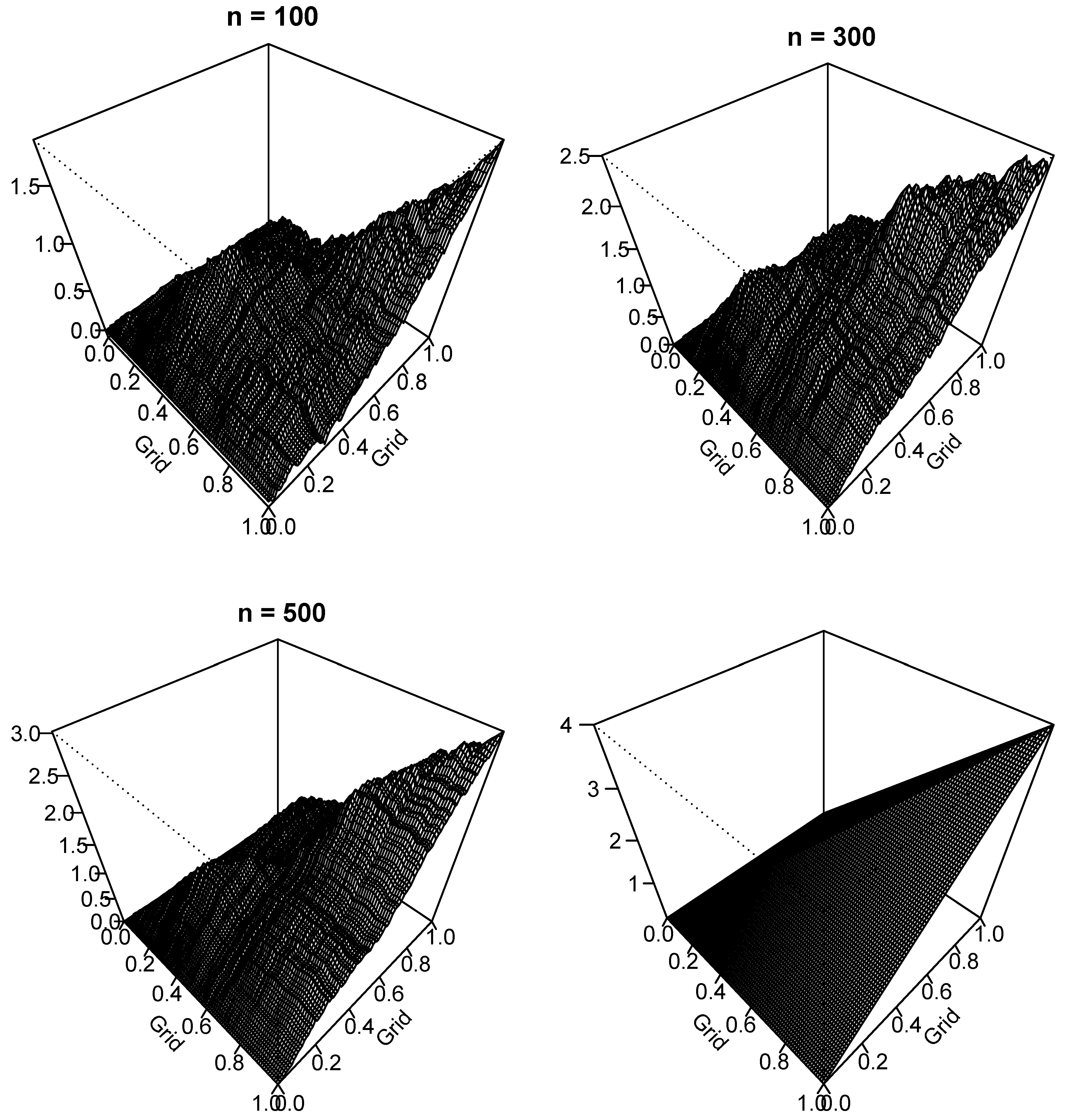
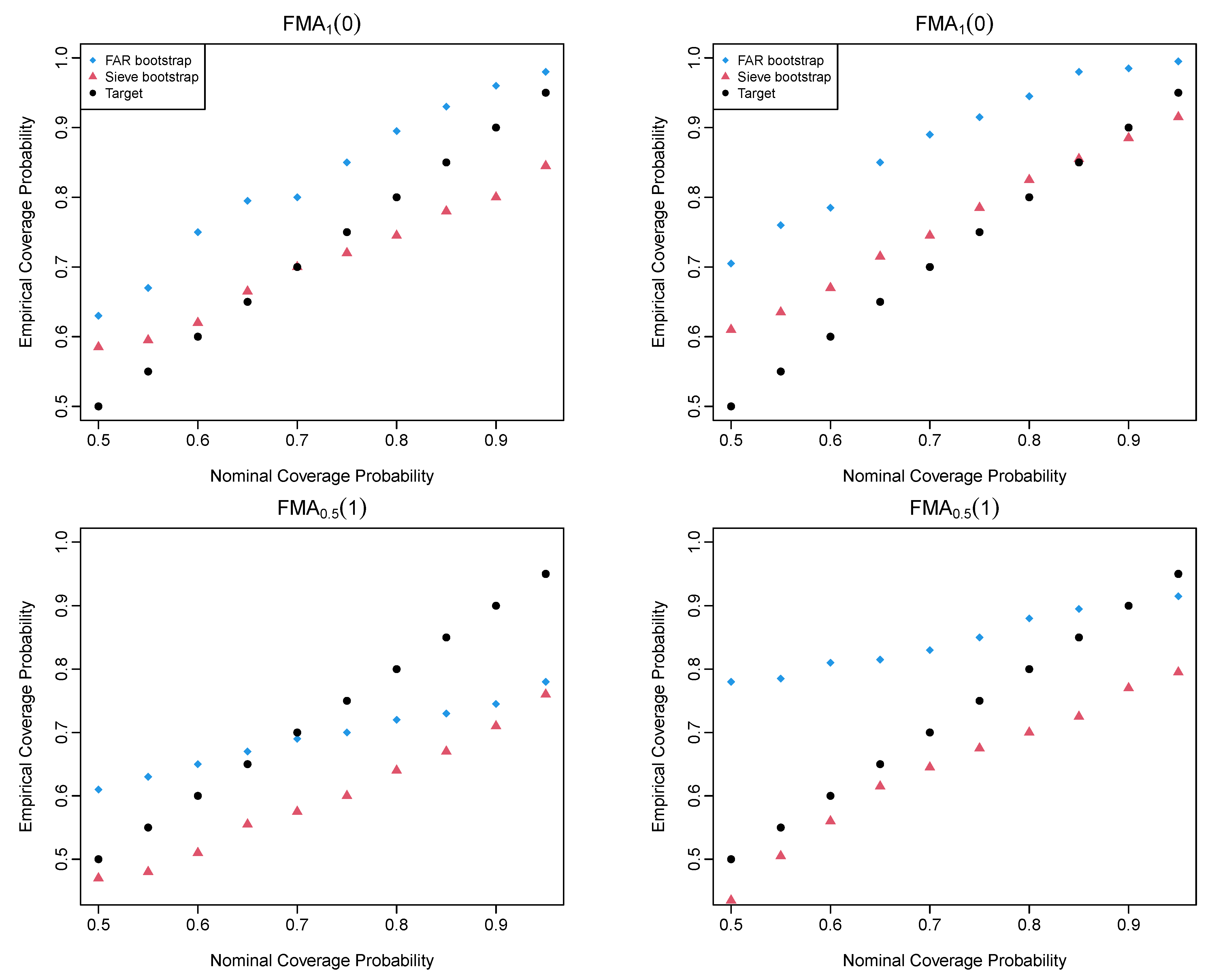
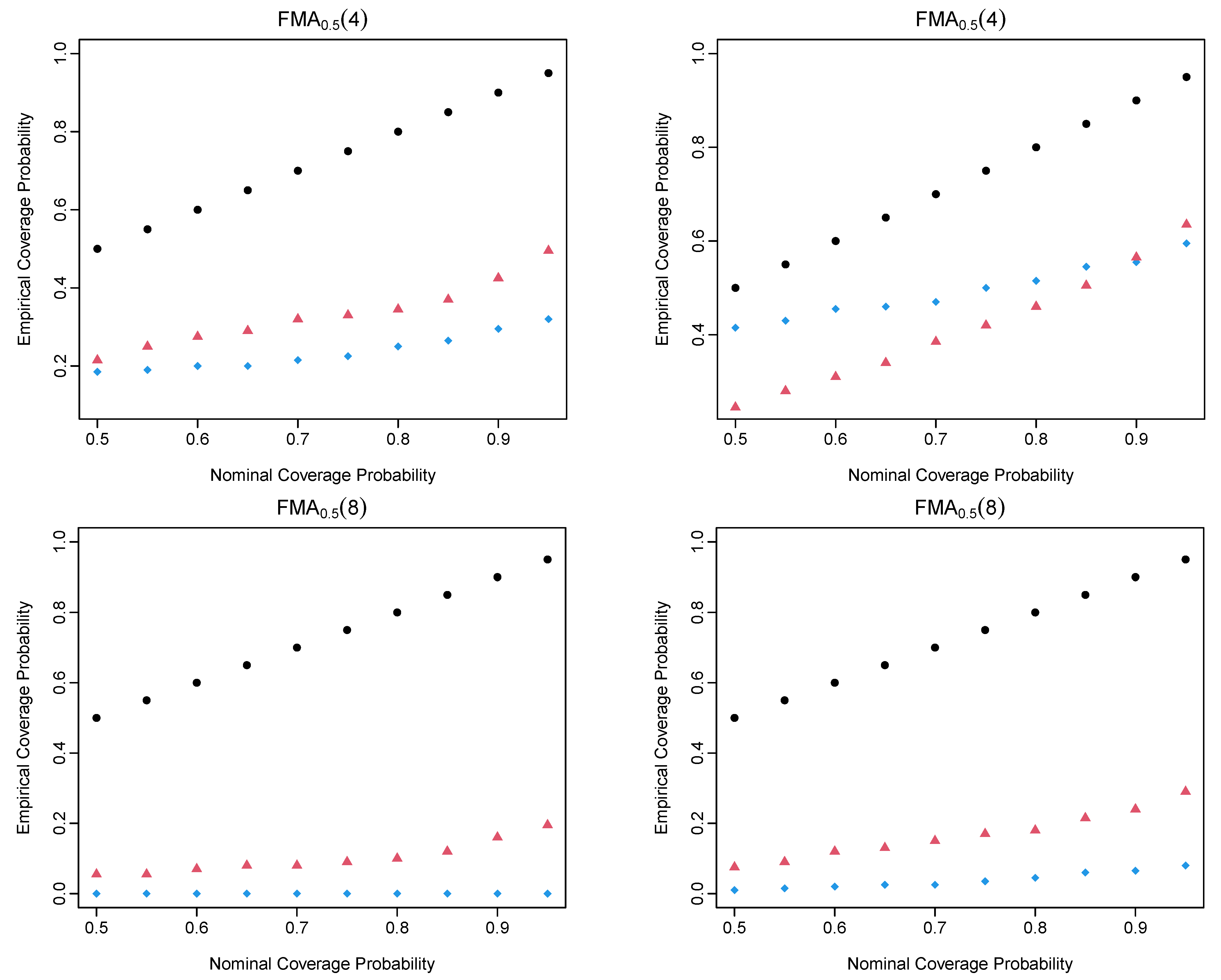
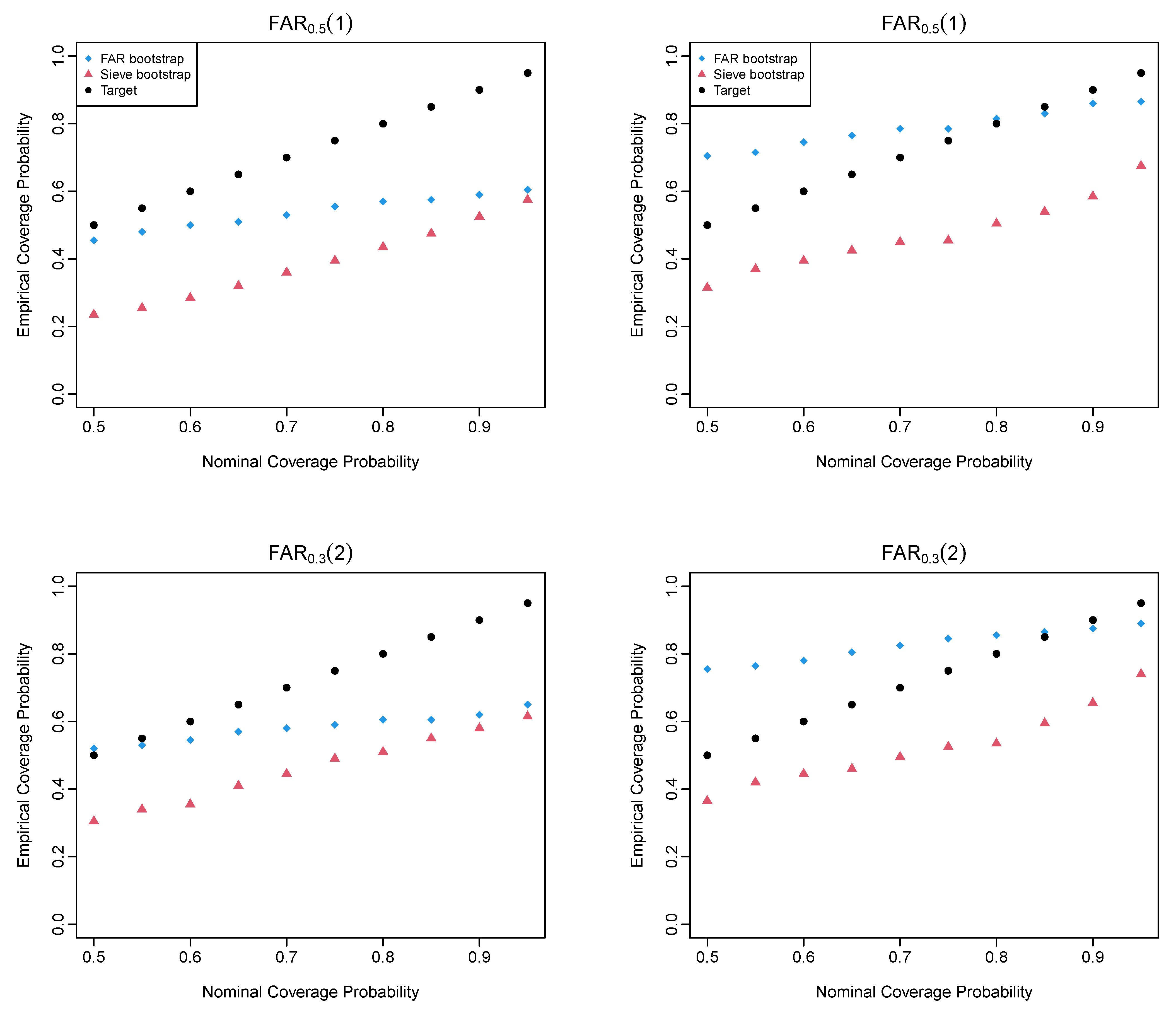
When the weakly stationarity condition satisfies for a functional time series $\{{\mathcal{X}}_1,\cdots ,{\mathcal{X}}_n\}$, a parametric estimator of the conditional mean can capture most of the correlation among functional time series. Among all parametric estimators, the FAR of order 1 is widely used; see [24], who derived one-step-ahead forecasts based on a regularized form of the Yule–Walker equations. We consider the FAR(1) model to estimate the conditional mean, and the model can be written as

$${\mathcal{X}}_t=\mu +\rho ({\mathcal{X}}_{t-1}-\mu )+{ϵ}_t,t=2,\cdots ,n,$$

where ${ϵ}_t$ denotes an error term with a mean of zero and $\rho =\mathrm{\Gamma }\left(1\right)/\mathrm{\Gamma }\left(0\right)$ represents the first-order autocorrelation operator. From a set of functional time series, the variance and first-order autocovariance functions $\mathrm{\Gamma }\left(0\right)$ and $\mathrm{\Gamma }\left(1\right)$ are estimated by the sample variance and autocovariance

$$\widehat{\mathrm{\Gamma }}\left(0\right)=\frac{1}{n}\sum _{t=1}^n{\mathcal{X}}_t^c\otimes {\mathcal{X}}_t^c,\widehat{\mathrm{\Gamma }}\left(1\right)=\frac{1}{n}\sum _{t=1}^{n-1}{\mathcal{X}}_t^c\otimes {\mathcal{X}}_{t+1}^c,$$

where ${\mathcal{X}}_t^c={\mathcal{X}}_t-\frac{1}{n}{\sum }_{t=1}^n{\mathcal{X}}_t$ and ⊗ denotes a tensor product which is a means of combining vectors from different Hilbert spaces to form a new vector in a larger Hilbert space.

When the FAR(1) model is the correct parametric model for modeling the underlying data-generating process, the best linear predictor of ${\mathcal{X}}_t^c$ given the past values ${\mathcal{X}}_{t-1}^c$ is given by

$${\widehat{\mathcal{X}}}_t^c=\widehat{\rho }{\mathcal{X}}_{t-1}^c,$$

where $\widehat{\rho }=\widehat{\mathrm{\Gamma }}\left(1\right)/\widehat{\mathrm{\Gamma }}\left(0\right)$. Since $\widehat{\mathrm{\Gamma }}\left(0\right)$ may be unbounded, a regularization technique, such as ridge estimator, can be adopted (see, e.g., [24]). The ridge estimator adds a random noise to the $\widehat{\mathrm{\Gamma }}\left(0\right)$ to make it invertible. The one-step-ahead residual function is then given by

$${\widehat{ϵ}}_t={\mathcal{X}}_t^c-{\widehat{\mathcal{X}}}_t^c,t=2,\cdots ,n.$$

Let ${\widehat{ϵ}}_t^c={\widehat{ϵ}}_t-\frac{1}{n-1}{\sum }_{t=2}^n{\widehat{ϵ}}_t$ be centered realizations of a stochastic process. The centering is important to ensure that the resulting bootstrap approximation is free of a random bias that does not vanish in the limit (see also [25]). The residual functions can be resampled with a replacement from the centered residual functions (see [13], Section 3.2 for more details).

4. Simulation Study

We introduce our simulation setup in Section 4.1, while the evaluation metrics are presented in Section 4.2. Simulation results for the FMA processes are shown in Section 4.3, while simulation results for the FAR processes are presented in Section 4.4.

4.1. Simulation Data Generating Processes (DGPs)

Let $\{B_t\left(u\right),-\infty <t<\infty ,u\in [0,1]\}$ denote i.i.d. standard Brownian motions. Following [18], we generate a set of stationary functional time series from the following DGPs

$$\begin{array}{cc}\hfill {\mathrm{FAR}}_{\varphi }\left(\omega \right):{\mathcal{X}}_t\left(u\right)& =\sum _{k=1}^{\omega }{\varphi }_k{\mathcal{X}}_{t-k}\left(u\right)+B_t\left(u\right)\hfill \\ \hfill {\mathrm{FMA}}_{\psi }\left(q\right):{\mathcal{X}}_t\left(u\right)& =B_t\left(u\right)+\psi \sum _{k=1}^q{B}_{t-k}\left(u\right),\hfill \end{array}$$

where ${\mathrm{FAR}}_{\varphi }\left(\omega \right)$ is the functional analog of an autoregressive process of order $\omega$, and ${\mathrm{FMA}}_{\psi }\left(q\right)$ is the functional analog of a moving average process of order q. The coefficients ${\varphi }_k$ and $\psi$ are scalar chosen to mimic various dependence structures. We consider a total of six DGPs: ${\mathrm{FAR}}_{0.5}\left(1\right)$, ${\mathrm{FAR}}_{(-0.6,0.09)}\left(2\right)$, ${\mathrm{FMA}}_1\left(0\right)$, ${\mathrm{FMA}}_{0.5}\left(1\right)$, ${\mathrm{FMA}}_{0.5}\left(4\right)$, ${\mathrm{FMA}}_{0.5}\left(8\right)$.

In Figure 1, we show perspective plots of the long-run covariance function estimates from a set of samples following the ${\mathrm{FAR}}_{0.5}\left(1\right)$ process. Using the kernel sandwich estimator in Section 2, we display the estimated long-run covariance function for $n=100, 300, 500$ and the theoretical long-run covariance.

We compute the Hilbert–Schmidt norm of the difference between the estimated and actual long-run covariance functions. For this simulated example, the values of the Hilbert–Schmidt norm are 114, 58, and 47 when n = 100, 300, and 500, respectively. As the sample size increases, the Hilbert–Schmidt norm decreases for this data-generating process. This phenomenon practically justifies the kernel sandwich estimator can consistently estimate the population long-run covariance function.

To assess the strength of temporal dependence, we compute a functional analog of the autocorrelation function (ACF), defined as

$$\frac{\parallel {\widehat{\gamma }}_{\ell }\parallel }{\int {\widehat{\gamma }}_0(t,t)dt},$$

where $\parallel ·\parallel$ denotes the $L_2$ norm. Unlike the univariate ACF, functional ACF only measures the strength of the temporal dependency since $\parallel {\widehat{\gamma }}_{\ell }\parallel \ge 0$. Proposed by [26], the functional ACF is a graphical indicator for the order selection of functional moving average (FMA) processes.

Table 1. Estimated functional ACF averaged over 200 replications for various DGPs.

DGP	${\mathrm{lag}}_1$	${\mathrm{lag}}_2$	${\mathrm{lag}}_3$	${\mathrm{lag}}_4$	${\mathrm{lag}}_5$
${\mathrm{FAR}}_{0.5}\left(1\right)$	0.3979	0.1967	0.1298	0.1172	0.1112
${\mathrm{FAR}}_{(-0.6,0.09)}\left(2\right)$	0.4396	0.1914	0.1242	0.1178	0.1140
${\mathrm{FMA}}_1\left(0\right)$	0.0923	0.0930	0.0912	0.0922	0.0959
${\mathrm{FMA}}_{0.5}\left(1\right)$	0.3961	0.1123	0.1113	0.1107	0.1153
${\mathrm{FMA}}_{0.5}\left(4\right)$	0.6365	0.4647	0.3055	0.1849	0.1653
${\mathrm{FMA}}_{0.5}\left(8\right)$	0.7068	0.5986	0.4974	0.4024	0.3134

presents the estimated functional ACF averaged over 200 replications for 6 DGPs. The DGPs exhibit different levels of dependence structures. When the process follows an ${\mathrm{FMA}}_1\left(0\right)$, the autocorrelations at all lags are similar. When the process follows an ${\mathrm{FMA}}_{0.5}\left(8\right)$, there is still a strong dependence even at lag 5, highlighting a strong persistence in the functional time series.

4.2. Simulation Evaluation Metrics

Let $\mathcal{C}=\psi \left({\mathcal{F}}_0\right)$ be the population long-run covariance whose distribution is unknown, where $\psi$ is the function that defines $\mathcal{C}$. Although the distribution of a statistic is unknown, we can approximate it by an empirical distribution of ${\mathcal{F}}_1$. Let ${\mathcal{X}}^{*}=({\mathcal{X}}_1^{*},{\mathcal{X}}_2^{*},\cdots ,{\mathcal{X}}_n^{*})$ be a set of bootstrap sample of size n drawn from the empirical distribution ${\mathcal{F}}_1$. Let ${\mathcal{F}}_1^{*}$ be the estimate of ${\mathcal{F}}_0$ re-computed from the bootstrap sample ${\mathcal{X}}^{*}$.

Let $D({\widehat{\mathcal{C}}}_n,\mathcal{C})$ be the distance of the long-run covariance functions between the population and sample levels. Let $D({\widehat{\mathcal{C}}}_n^{*},{\widehat{\mathcal{C}}}_n)$ be the distance of the long-run covariance functions between the original and bootstrap samples.

To evaluate the finite-sample performance of the bootstrap procedures, we compute the bootstrap CIs of the long-run covariance. As a performance measure, ${\mathcal{L}}^2$ distance metrics are used for constructing CIs. The Hilbert–Schmidt norm is defined as

$$\begin{array}{cc}\hfill T_n& \equiv {∥\mathcal{C}(u,v)-{\widehat{\mathcal{C}}}_n(u,v)∥}_{\mathrm{HS}}\hfill \\ \hfill & ={\left\{{\int }_{u\in \mathcal{I}}{\int }_{v\in \mathcal{I}}{\left[\mathcal{C}(u,v)-\widehat{\mathcal{C}}(u,v)\right]}^{2}dudv\right\}}^{\frac{1}{2}}.\hfill \end{array}$$

(4)

Given a set of original functions $\{{\mathcal{X}}_1,{\mathcal{X}}_2,\cdots ,{\mathcal{X}}_n\}$, we draw $B=400$ bootstrap samples for each of the $R=200$ replications. The same pseudo-random seed was used for all the procedures to ensure the same simulation randomness. We compute the Hilbert–Schmidt norm of the difference between the bootstrap and sample long-run covariance functions for each replication. By sorting the norm values, we find a threshold value, denoted by $T_n^{*,\mathrm{threshold}}$, that $100(1-\alpha )\%$ of the norm values are included.

Based on 200 replications, we compute the empirical coverage probability as $\frac{1}{200}{\sum }_{r=1}^{200}{I}_r$, where $I_r=\mathbb{1}(T_n^{*,\mathrm{threshold}}\le T_n)$ and $\mathbb{1}\{·\}$ denotes a binary indicator function. Our evaluation procedure presents a partial view by only showing only the distributional approximation of $\parallel C(u,v)-{\widehat{C}}_n{(u,v)\parallel }_{\mathrm{HS}}$ by $\parallel {\widehat{C}}_n^{*}(u,v)-{\widehat{C}}_n{(u,v)\parallel }_{\mathrm{HS}}$ instead of the distributional approximation of ${\widehat{C}}_n(u,v)-C(u,v)$ by ${\widehat{C}}_n^{*}(u,v)-{\widehat{C}}_n(u,v)$. Due to the infinite dimensionality of functional data, some estimators of an infinite-dimensional parameter may not have an asymptotic result [27].

4.3. Simulation Results of the FMA Processes

Based on the Hilbert–Schmidt norm introduced in (4), we could determine the empirical coverage probability, calculated as the ratio of the number of observations that fall into the constructed confidence intervals to the total number of observations. For a range of nominal coverage probabilities from 0.5 to 0.95 in a step of 0.05, we display the nominal and empirical coverage probabilities in Figure 2 for the four chosen FMA processes. As the order of FMA processes increases from lag 0 to 8, it becomes more difficult to estimate the long-run covariance function with the same sample size.

The sieve bootstrap is the method that follows comparably close to the nominal coverage probabilities. We calculate the coverage probability difference (CPD), the absolute difference between the empirical and nominal coverage probabilities. In

Table 2. When the data-generating processes are the FMA processes, we compute the averaged CPD over a set of nominal coverage probabilities from 0.5 to 0.95 in a step of 0.05 between the FAR and sieve bootstrap methods.

	$\mathit{n}=100$		$\mathit{n}=300$
	FAR Bootstrap	Sieve Bootstrap	FAR Bootstrap	Sieve Bootstrap
${\mathrm{FMA}}_1\left(0\right)$	0.1010	0.0525	0.1560	0.0490
${\mathrm{FMA}}_{0.5}\left(1\right)$	0.0845	0.1280	0.1280	0.0825
${\mathrm{FMA}}_{0.5}\left(4\right)$	0.4905	0.3935	0.2310	0.3105
${\mathrm{FMA}}_{0.5}\left(8\right)$	0.7250	0.6245	0.6870	0.5590

, we present the average CPD values over a set of nominal coverage probabilities ranging from 0.5 to 0.95 in a step of 0.05. For the four FMA processes, the sieve bootstrap is generally recommended. The bootstrap methods produce relatively large CPD values as the temporal dependence increases. As the sample size n increases, the performance of the sieve bootstrap improves, but it is not necessary for the FAR bootstrap. A possible reason is the model misspecification issue between the chosen model and the data-generating process.

4.4. Simulation Results of the FAR Processes

In Figure 3, we display the nominal and empirical coverage probabilities for estimating the long-run covariance of stationary functional time series among the bootstrap methods. We consider two FAR processes in which the serial dependence changes from FAR$\left(1\right)$ to FAR$\left(2\right)$. The FAR bootstrap method is recommended between the two bootstrap methods.

From Figure 3 and

Table 3. When the data-generating processes are the FAR processes, we compute the averaged CPD over a set of nominal coverage probabilities from 0.5 to 0.95 in a step of 0.05 among the FAR and sieve bootstrap methods.

	$\mathit{n}=100$		$\mathit{n}=300$
	FAR Bootstrap	Sieve Bootstrap	FAR Bootstrap	Sieve Bootstrap
${\mathrm{FAR}}_{0.5}\left(1\right)$	0.1880	0.3390	0.0910	0.2535
${\mathrm{FAR}}_{-0.6,0.09}\left(2\right)$	0.1475	0.2650	0.1180	0.2015

, the FAR bootstrap is the method that follows comparably close to the nominal coverage probabilities. When FAR(1) is the true data-generating process, the FAR bootstrap is expected to perform the best. When the model is misspecified, the FAR bootstrap still outperforms the sieve bootstrap, reflecting some degree of model robustness. From the averaged CPD values, the FAR bootstrap is recommended with the smallest values for the two FAR processes. As the sample size increases from $n=100$ to 300, the CPD values decrease for the bootstrap methods.

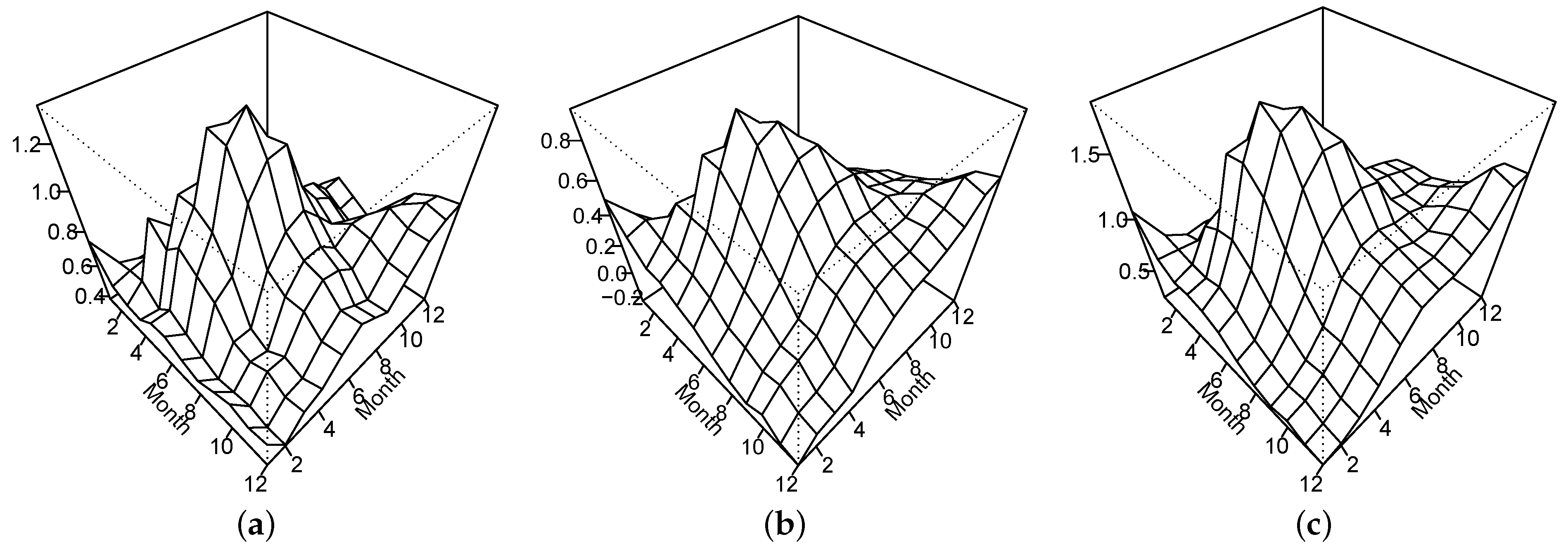
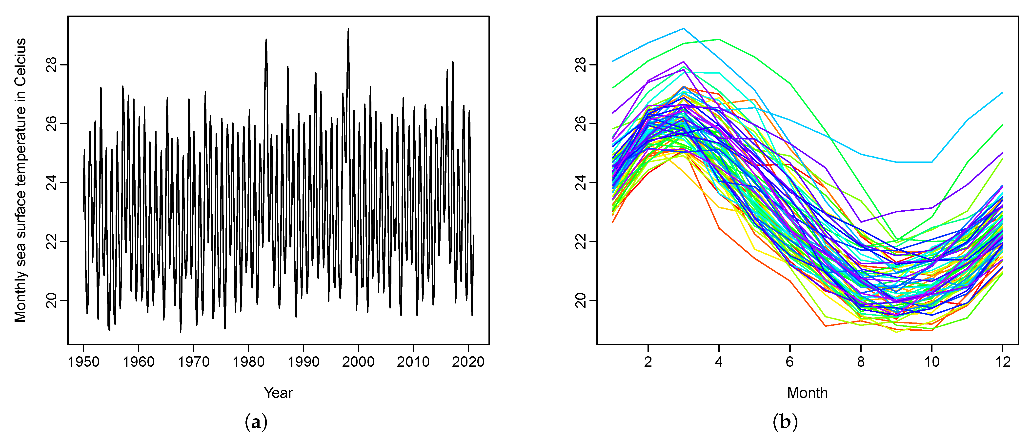
5. Monthly Sea Surface Temperature

We consider a time series of average monthly sea surface temperatures in degrees Celsius from January 1950 to December 2020, available online at https://www.cpc.ncep.noaa.gov/data/indices/ersst5.nino.mth.91-20.ascii (accessed on 31 January 2024). These sea surface temperatures are measured by moored buoys in the “Niño region” defined by the coordinates 0–${10}^{\circ }$ South and ${90}^{\circ }$–${80}^{\circ }$, West. In this case, each curve represents one year of observed sea surface temperatures. There are $N=852$ discrete univariate time series data points, which are converted into $n=71$ monthly curves. The discretized functional time series, which consists of $\delta =\lfloor N/n\rfloor$ discrete data points, is given by

$${\mathcal{X}}_t\left(u_i\right)=\{x_w,w\in (\delta (t-1),\delta t]\},t=1,2,\cdots ,n,$$

where $i=1,2,\cdots ,12$ denotes 12 discrete data points within a year. A univariate time series display of the monthly sea surface temperature is given in Figure 4a, with the same data shown in Figure 4b as a time series of functions.

We examine the stationarity assumption of this dataset by applying a test procedure of [28]. Under the null hypothesis that the functional time series is stationary, based on the p-value of 0.684, we cannot reject the null hypothesis at the customarily 5% level of significance.

We apply the sieve bootstrap method to construct 80% confidence intervals of the long-run covariance function of the dataset. The sample estimated long-run covariance is shown in Figure 5a, and the lower and upper bounds of the 80% CIs are shown in Figure 5b and Figure 5c, respectively.

6. Conclusions

We apply two bootstrap methods, namely the sieve and FAR bootstrap methods, to generate bootstrap samples of stationary functional time series. Via a series of simulation studies, we study several data-generating processes for stationary functional time series. The data-generating processes can be split into the FMA and FAR processes. We compute the distance between the sample and population long-run covariance functions for each data-generating process. For each bootstrap sample, we estimate its long-run covariance function and compute its distance from the sample’s long-run covariance. With the two distances from 200 replications, we compute empirical coverage probability for a set of nominal coverage probabilities ranging from 0.5 to 0.95 in a step of 0.05. The sieve bootstrap is generally recommended when the data-generating process is generated from the FMA processes. The FAR bootstrap is advocated when the data-generating process stems from the FAR processes. To determine whether a functional time series is generated from a FAR process, one can apply a hypothesis test of [29].

Our finding highlights the importance of model specification for stationary functional time series and further confirms the estimation difficulty associated with strongly dependent functional time series. The bootstrap validity hinges on the existence of the fourth-order moment and works for Gaussian processes. If the underlying process is non-Gaussian, the bootstrap is known to fail (cf. [30,31]). This is because the variance of the limiting distributions depends on the fourth-order cumulants; the bootstrap may not approximate these fourth-order cumulants. The hypothesis tests of [32] are useful for testing the normality of functional time series. In future research, one may develop hypothesis tests to examine whether or not a stochastic process is generated from a heavy-tailed distribution with an infinite second or fourth moment.

References

1. Hörmann, S.; Kokoszka, P. Functional time series. In Handbook of Statistics; Rao, T.S., Rao, S.S., Eds.; Elsevier: Amsterdam, The Netherlands, 2012; Volume 30, pp. 157–186. [Google Scholar]
2. Kokoszka, P.; Rice, G.; Shang, H.L. Inference for the autocovariance of a functional time series under conditional heteroscedasticity. J. Multivar. Anal. 2017, 162, 32–50. [Google Scholar] [CrossRef]
3. Andersen, T.G.; Su, T.; Todorov, V.; Zhang, Z. Intraday periodic volatility curves. J. Am. Stat. Assoc. Theory Methods 2023, in press. [Google Scholar] [CrossRef]
4. Ferraty, F.; Vieu, P. Nonparametric Functional Data Analysis: Theory and Practice; Springer: Berlin/Heidelberg, Germany, 2006. [Google Scholar]
5. Ramsay, J.O.; Silverman, B.W. Functional Data Analysis; Springer: New York, NY, USA, 2005. [Google Scholar]
6. Kokoszka, P.; Reimherr, M. Introduction to Functional Data Analysis; CRC Press: Boca Raton, FL, USA, 2017. [Google Scholar]
7. Peña, D.; Tsay, R.S. Statistical Learning for Big Dependent Data; Wiley: Hoboken, NJ, USA, 2021. [Google Scholar]
8. Politis, D.N. The impact of bootstrap methods on time series analysis. Stat. Sci. 2003, 18, 219–230. [Google Scholar] [CrossRef]
9. Hörmann, S.; Kidzinski, L.; Hallin, M. Dynamic functional principal components. J. R. Stat. Soc. Ser. B 2015, 77, 319–348. [Google Scholar] [CrossRef]
10. Franke, J.; Nyarige, E.G. A residual-based bootstrap for functional autoregressions. Working paper, Technische Universität Kaiserslautern. arXiv 2019, arXiv:abs/1905.07635. [Google Scholar]
11. Nyarige, E.G. The Bootstrap for the Functional Autoregressive Model FAR(1). Ph.D. Thesis, Technische Universität Kaiserslautern, Kaiserslautern, Germany, 2016. Available online: https://kluedo.ub.uni-kl.de/frontdoor/index/index/year/2016/docId/4410 (accessed on 31 January 2023).
12. Pilavakis, D.; Paparoditis, E.; Sapatinas, T. Moving block and tapered block bootstrap for functional time series with an application to the K-sample mean problem. Bernoulli 2019, 25, 3496–3526. [Google Scholar] [CrossRef]
13. Shang, H.L. Bootstrap methods for stationary functional time series. Stat. Comput. 2018, 28, 1–10. [Google Scholar] [CrossRef]
14. Paparoditis, E. Sieve bootstrap for functional time series. Ann. Stat. 2018, 46, 3510–3538. [Google Scholar] [CrossRef]
15. Ferraty, F.; Vieu, P. Kernel regression estimation for functional data. In The Oxford Handbook of Functional Data Analysis; Ferraty, F., Ed.; Oxford University Press: Oxford, UK, 2011; pp. 72–129. [Google Scholar]
16. Zhu, T.; Politis, D.N. Kernel estimates of nonparametric functional autoregression models and their bootstrap approximation. Electron. J. Stat. 2017, 11, 2876–2906. [Google Scholar] [CrossRef]
17. Paparoditis, E.; Shang, H.L. Bootstrap prediction bands for functional time series. J. Am. Stat. Assoc. Theory Methods 2023, 118, 972–986. [Google Scholar] [CrossRef]
18. Rice, G.; Shang, H.L. A plug-in bandwidth selection procedure for long run covariance estimation with stationary functional time series. J. Time Ser. Anal. 2017, 38, 591–609. [Google Scholar] [CrossRef]
19. Franke, J.; Hardle, W. On bootstrapping kernel spectral estimate. Ann. Stat. 1992, 20, 121–145. [Google Scholar] [CrossRef]
20. Politis, D.N.; Romano, J.P. On flat-top spectral density estimators for homogeneous random fields. J. Stat. Plan. Inference 1996, 51, 41–53. [Google Scholar] [CrossRef]
21. Li, D.; Robinson, P.M.; Shang, H.L. Long-range dependent curve time series. J. Am. Stat. Assoc. Theory Methods 2020, 115, 957–971. [Google Scholar] [CrossRef]
22. Ahn, S.C.; Horenstein, A.R. Eigenvalue ratio test for the number of factors. Econometrica 2013, 81, 1203–1227. [Google Scholar]
23. Hurvich, C.M.; Tsai, C.-L. A corrected Akaike information criterion for vector autoregressive model selection. J. Time Ser. Anal. 1993, 14, 271–279. [Google Scholar] [CrossRef]
24. Bosq, D. Linear Processes in Function Spaces; Lecture notes in Statistics; Springer: New York, NY, USA, 2000. [Google Scholar]
25. Lahiri, S.N. Resampling Methods for Dependent Data; Springer: New York, NY, USA, 2003. [Google Scholar]
26. Mestre, G.; Portela, J.; Rice, G.; Roque, A.M.S.; Alonso, E. Functional time series model identification and diagnosis by means of auto- and partial autocorrelation analysis. Comput. Stat. Data Anal. 2021, 155, 107108. [Google Scholar] [CrossRef]
27. Cardot, H.; Mas, A.; Sarda, P. CLT in functional linear regression models. Probab. Theory Relat. Fields 2007, 138, 325–361. [Google Scholar] [CrossRef]
28. Horváth, L.; Kokoszka, P.; Rice, G. Testing stationarity of functional time series. J. Econom. 2014, 179, 66–82. [Google Scholar] [CrossRef]
29. Kokoszka, P.; Reimherr, M. Determining the order of the functional autoregressive model. J. Time Ser. Anal. 2013, 34, 116–129. [Google Scholar] [CrossRef]
30. Kreiss, J.-P.; Paparoditis, E.; Politis, D.N. On the range of validity of the autoregressive sieve bootstrap. Ann. Stat. 2011, 39, 2103–2130. [Google Scholar]
31. Paparoditis, E.; Meyer, M.; Kreiss, J.-P. Extending the validity of frequency domain bootstrap methods to general stationary processes. Annals of Statistics 2020, 48, 2404–2427. [Google Scholar]
32. Górecki, T.; Hörmann, S.; Horváth, L.; Kokoszka, P. Testing normality of functional time series. J. Time Ser. Anal. 2018, 39, 471–487. [Google Scholar] [CrossRef]
Figure 1. Three-dimensional perspective plots of the long-run covariance function estimators with simulated data from the FAR 0.5 ( 1 ) model using the sandwich estimator with a plug-in bandwidth selection method of [18] for sample sizes of n = 100, 300, and 500 along with the theoretical long-run covariance (lower right).
Forecasting 06 00008 g001
Figure 2. Empirical vs. nominal coverage probabilities of the four FMA processes when n = 100 (left column) and n = 300 (right column).
Forecasting 06 00008 g002aForecasting 06 00008 g002b
Figure 3. Empirical vs. nominal coverage probability of the FAR processes when n = 100 (left column) and n = 300 (right column).
Forecasting 06 00008 g003
Figure 4. Graphical displays of monthly measurements of the sea surface temperatures from January 1950 to December 2020: (a) a univariate time series display; (b) a functional time series display via rainbow plot. The curves in the distant past are shown in red, while the most recent curves are shown in purple.
Forecasting 06 00008 g004
Figure 5. Sample long-run covariance function estimated by the kernel sandwich estimator, and the estimated 80% lower and upper bounds of the estimated long-run covariance function: (a) sample; (b) lower bound; and (c) upper bound.
Forecasting 06 00008 g005