Model-Free Time-Aggregated Predictions for Econometric Datasets

Abstract

Forecasting volatility from econometric datasets is a crucial task in finance. To acquire meaningful volatility predictions, various methods were built upon GARCH-type models, but these classical techniques suffer from instability of short and volatile data. Recently, a novel existing normalizing and variance-stabilizing (NoVaS) method for predicting squared log-returns of financial data was proposed. This model-free method has been shown to possess more accurate and stable prediction performance than GARCH-type methods. However, whether this method can sustain this high performance for long-term prediction is still in doubt. In this article, we firstly explore the robustness of the existing NoVaS method for long-term time-aggregated predictions. Then, we develop a more parsimonious variant of the existing method. With systematic justification and extensive data analysis, our new method shows better performance than current NoVaS and standard GARCH(1,1) methods on both short- and long-term time-aggregated predictions. The success of our new method is remarkable since efficient predictions with short and volatile data always carry great importance. Additionally, this article opens potential avenues where one can design a model-free prediction structure to meet specific needs.

1. Introduction

Accurate and robust volatility forecasting is a central focus in financial econometrics. This type of forecasting is crucial for practitioners and traders to make decisions in risk management, asset allocation, pricing of derivative instruments and strategic decisions regarding fiscal policies, etc. Standard methods to perform volatility forecasting are typically built upon applying GARCH-type models to predict squared financial log-returns. With the model-free prediction principle, first proposed by Politis [1], a model-free volatility prediction method—NoVaS—has been proposed recently for efficient forecasting without the assumption of normality. Some previous studies have shown that the NoVaS method possesses better predictive performance than GARCH-type models when forecasting squared log-returns, e.g., Gulay and Emec [2] showed that the NoVaS method could overcome GARCH-type models (GARCH, EGARCH and GJR-GARCH) with generalized error distributions by comparing the pseudo-out-of-sample (POOS) forecasting performance on S&P500 and BIST 100 return series (here the pseudo-out-of-sample forecasting analysis means using data up to and including the current time to predict future values). Chen and Politis [3] showed that the “time-varying” NoVaS method is robust against possible non-stationarities in the data. Furthermore, Chen and Politis [4] extended this NoVaS approach to perform multi-step-ahead predictions of squared log-returns.

However, to the best of our knowledge, such methods have not been evaluated for time-aggregated prediction. Time-aggregated prediction here stands for the prediction of $Y_{n+1}+\cdots +Y_{n+h}$ after observing ${\left\{Y_t\right\}}_{t=1}^n$. Such predictions remain crucial for strategic decisions implemented by commodity or service providers, ([5,6]), trust funds, pension management, insurance companies, portfolio management of specific derivatives ([7]) and assets ([8]). Time-aggregated forecasting is also able to provide some degree of confidence in understanding the general trend in the near future, potentially for the entire following week or months ahead, which is definitely more meaningful than merely understanding what might happen for any single step ahead (predicting $Y_{n+h}$ for one value of h) in the time horizon. In fact, the quality of forecasts for econometric data has been evaluated through such time-aggregated metrics in [9,10]. In this article, we continue utilizing these time-aggregated metrics to challenge the ability of the NoVaS method for short- and long-term time-aggregated predictions on squared log-returns series. For exploring such capabilities of the existing NoVaS method, we set up comprehensive data analyses to substantiate the efficiency of the NoVaS method and also address the lack of data experiments in NoVaS studies. Apart from this, we also attempt to improve the existing one further by proposing a more parsimonious model. Based on extensive data analysis, our new method shows more stable performance than the state-of-the-art NoVaS method regardless of whether simulation or real-world data are used. We also find that the state-of-the-art NoVaS method is even surpassed by the standard GARCH(1,1) model sometimes. On the other hand, our new method returns consistently excellent forecasting. Notably, our method achieves a remarkable improvement when the dataset at hand is short and volatile.

The rest of this article is organized as follows. In Section 2, we firstly introduce the theoretical background and structure of the existing NoVaS method. Then, our new method is proposed and a simple comparison is made to show the stability of our new method. In Section 3, we substantiate our proposal by extensive simulations and data analysis. Moreover, we utilize the CW test to support our parsimonious model. Finally, a summary and discussion are given in Section 4 and Section 5, respectively.

2. Method

2.1. The Existing NoVaS Method

The NoVaS method is a model-free prediction principle. The main idea lies in applying an invertible transformation H, which can map the non-$i.i.d$. vector ${\left\{Y_i\right\}}_{i=1}^t$ to a vector ${\left\{{ϵ}_i\right\}}_{i=1}^t$ that has $i.i.d.$ components. This leads to the prediction of $Y_{t+1}$ by inversely transforming the prediction of ${ϵ}_{t+1}$ [11]. The starting point to build the transformation of the existing NoVaS method is the ARCH model [12]. Then, Politis [1] made some adjustments to determine the final form of H as:

$$W_t=\frac{Y_t}{\sqrt{\alpha s_{t-1}^2+{\tilde{a}}_0{Y}_t^2+{\sum }_{i=1}^p{a}_i{Y}_{t-i}^2}}\mathrm{for}t=p+1,\cdots ,n.$$

(1)

In Equation (1), ${\left\{Y_t\right\}}_{t=1}^n$ is the log-returns vector in this article; ${\left\{W_t\right\}}_{t=p+1}^n$ is the transformed vector, which we hope to transform to $i.i.d.$; $\alpha$ is a fixed-scale invariant constant; $s_{t-1}^2$ is calculated by ${(t-1)}^{-1}{\sum }_{i=1}^{t-1}{(Y_i-\mu )}^2$, with $\mu$ being the mean of ${\left\{Y_i\right\}}_{i=1}^{t-1}$; ${\tilde{a}}_0$ is the coefficient corresponding with the currently observed value $Y_t^2$. For reaching a qualified transformation function, Equation (2) is required to stabilize the variance.

$$\alpha \in (0,1),{\tilde{a}}_0\ge 0,a_i\ge 0\mathrm{for}\mathrm{all}i\ge 1,\alpha +{\tilde{a}}_0+\sum _{i=1}^p{a}_i=1$$

(2)

Then, $\alpha$ and ${\tilde{a}}_0,a_1,\cdots ,a_p$ are finally determined by minimizing $\left|Kurtosis\right(W_t)-3|$. In practice, the transformed $\left\{W_t\right\}$ is usually uncorrelated; see [11] for additional processes for correlated $\left\{W_t\right\}$. This method is model-free in the sense that we do not assume any particular distribution for the innovation $\left\{W_t\right\}$ except for matching its kurtosis to 3. Once H is found, $H^{-1}$ can be obtained immediately. For example, $H^{-1}$ corresponding with Equation (1) is:

$$Y_t=\sqrt{\frac{W_t^2}{1-{\tilde{a}}_0{W}_t^2}(\alpha s_{t-1}^2+\sum _{i=1}^p{a}_i{Y}_{t-i}^2)}\mathrm{for}t=p+1,\cdots ,n.$$

(3)

To obtain the prediction of $Y_{n+1}^2$, Politis [11] defined two types of optimal predictors under $L_1$ (Mean Absolute Deviation) and $L_2$ (Mean Squared Error) criteria after observing historical information set ${\mathcal{F}}_n=\{Y_t,1\le t\le n\}$:

$$\begin{array}{cc}\hfill L_1-\mathrm{optimal}\mathrm{predictor}\mathrm{of}& Y_{n+1}^2:\hfill \\ & \mathrm{Median}\left\{Y_{n+1,m}^2:m=1,\cdots ,M|{\mathcal{F}}_n\right\}\hfill \\ \hfill & =\mathrm{Median}\left\{\frac{W_{n+1,m}^2}{1-{\tilde{a}}_0{W}_{n+1,m}^2}(\alpha s_n^2+\sum _{i=1}^p{a}_i{Y}_{n+1-i}^2):m=1,\cdots ,M|{\mathcal{F}}_n\right\}\hfill \\ \hfill & =(\alpha s_n^2+\sum _{i=1}^p{a}_i{Y}_{n+1-i}^2)\mathrm{Median}\left\{\frac{W_{n+1,m}^2}{1-{\tilde{a}}_0{W}_{n+1,m}^2}:m=1,\cdots ,M\right\}\hfill \\ \hfill L_2-\mathrm{optimal}\mathrm{predictor}\mathrm{of}& Y_{n+1}^2:\hfill \\ \hfill & \mathrm{Mean}\left\{Y_{n+1,m}^2:m=1,\cdots ,M|{\mathcal{F}}_n\right\}\hfill \\ \hfill & =\mathrm{Mean}\left\{\frac{W_{n+1,m}^2}{1-{\tilde{a}}_0{W}_{n+1,m}^2}(\alpha s_n^2+\sum _{i=1}^p{a}_i{Y}_{n+1-i}^2):m=1,\cdots ,M|{\mathcal{F}}_n\right\}\hfill \\ \hfill & =(\alpha s_n^2+\sum _{i=1}^p{a}_i{Y}_{n+1-i}^2)\mathrm{Mean}\left\{\frac{W_{n+1,m}^2}{1-{\tilde{a}}_0{W}_{n+1,m}^2}:m=1,\cdots ,M\right\}\hfill \end{array}$$

(4)

where ${\left\{W_{n+1,m}\right\}}_{m=1}^M$ are generated M times from its empirical distribution or a normal distribution. Here, the normal distribution is an asymptotic limit of the empirical distribution of $\left\{W_{n+1}\right\}$. More details about this procedure and multi-step prediction are presented in Section 2.2. ${\left\{Y_{n+1,m}^2\right\}}_{m=1}^M$ are given by plugging ${\left\{W_{n+1,m}\right\}}_{m=1}^M$ into Equation (3) and setting t as $n+1$. During the optimization process, different forms of unknown parameters in Equation (2) are applied so that various NoVaS methods are established. Chen [13] pointed out that the Generalized Exponential NoVaS (GE-NoVaS) method with exponentially decayed unknown parameters presented in Equation (5) is superior to other NoVaS-type methods.

$$\alpha \ne 0,{\tilde{a}}_0=c^{\prime },a_i=c^{\prime }{e}^{-ci}\mathrm{for}\mathrm{all}1\le i\le p,c^{\prime }=\frac{1-\alpha }{{\sum }_{i=0}^p{e}^{-ci}}$$

(5)

2.2. A New Method with Less Parameters

However, during our investigation, we found that the GE-NoVaS method returns extremely large predictions under the $L_2$ criterion sometimes. The reason for this phenomenon is that the denominator of Equation (3) will be quite small when the generated $\left\{W^{*}\right\}$ (from empirical or normal distribution) is very close to $1/{\tilde{a}}_0$. In this situation, the prediction error will be amplified. Moreover, when the long-term ahead prediction is desired, this amplification will be accumulated and the final prediction will be dampened. Therefore, a removing-${\tilde{a}}_0$ idea is proposed to avoid such issues in this article. H and $H^{-1}$ of the GE-NoVaS-without-${\tilde{a}}_0$ method can be rewritten as below:

$$W_t=\frac{Y_t}{\sqrt{\alpha s_{t-1}^2+{\sum }_{i=1}^p{a}_i{Y}_{t-i}^2}};Y_t=\sqrt{W_t^2(\alpha s_{t-1}^2+\sum _{i=1}^p{a}_i{Y}_{t-i}^2)};\mathrm{for}t=p+1,\cdots ,n.$$

(6)

We should notice that even without the ${\tilde{a}}_0$ term, the causal prediction rule is still satisfied. It is easy to obtain the analytical form of the first-step-ahead $Y_{n+1}$, which can be expressed as below:

$$Y_{n+1}=\sqrt{W_{n+1}^2(\alpha s_n^2+\sum _{i=1}^p{a}_i{Y}_{n+1-i}^2)}$$

(7)

More specifically, when the first-step GE-NoVaS-without-${\tilde{a}}_0$ prediction is performed, $\left\{W_{n+1}^{*}\right\}$ are generated M (i.e., 5000 in this article) times from a standard normal distribution by the Monte Carlo method or bootstrapped from its empirical distribution ${\widehat{F}}_w$ which is calculated from Equation (1). Then, plugging these ${\left\{W_{n+1,m}^{*}\right\}}_{m=1}^M$ into Equation (7), M pseudo-predictions ${\left\{{\widehat{Y}}_{n+1,m}^{*}\right\}}_{m=1}^M$ are obtained. According to the strategy implied by Equation (4), we choose $L_1$ and $L_2$ risk optimal predictors ${\widehat{Y}}_{n+1}^2$ as the sample median and mean of $\{{\widehat{Y}}_{n+1,1}^{*},\cdots ,{\widehat{Y}}_{n+1,M}^{*}\}$, respectively. We can even predict the general form of $Y_{n+h}$, such as $g\left(Y_{n+h}\right)$, by adopting the sample mean or median of $\{g\left({\widehat{Y}}_{n+1,1}^{*}\right),\cdots ,g\left({\widehat{Y}}_{n+1,M}^{*}\right)\}$. Similarly, the two-steps-ahead $Y_{n+2}$ can be expressed as:

$$Y_{n+2}=\sqrt{W_{n+2}^2(\alpha s_{n+1}^2+a_1{Y}_{n+1}^2+\sum _{i=2}^p{a}_i{Y}_{n+2-i}^2)}$$

(8)

When the prediction of $Y_{n+2}$ is required, M pairs of $\{W_{n+1}^{*},W_{n+2}^{*}\}$ are still generated by bootstrapping or Monte Carlo method from empirically or standard normal distributions, respectively. $Y_{n+1}^2$ is replaced by the predicted value ${\widehat{Y}}_{n+1}^2$ which is derived from running the first-step GE-NoVaS-without-${\tilde{a}}_0$ prediction with simulated ${\left\{W_{n+1,m}^{*}\right\}}_{m=1}^M$ under the $L_1$ or $L_2$ criterion. Subsequently, we choose $L_1$ and $L_2$ risk optimal predictors of $Y_{n+2}$ as the sample median and mean of $\{{\widehat{Y}}_{n+2,1}^{*},\cdots ,{\widehat{Y}}_{n+2,M}^{*}\}$.

Finally, iterating the process described above, we can accomplish multi-step-ahead NoVaS predictions. $Y_{n+h},h\ge 3$ can be expressed as:

$$Y_{n+h}=\sqrt{W_{n+h}^2(\alpha s_{n+h-1}^2+\sum _{i=1}^p{a}_i{Y}_{n+h-i}^2)}$$

(9)

To obtain the prediction of $Y_{n+h}$, we generate M number of $\{W_{n+1}^{*},\cdots ,W_{n+h}^{*}\}$ and plug ${\left\{Y_{n+k}\right\}}_{k=1}^{h-1}$ with NoVaS predicted values ${\left\{{\widehat{Y}}_{n+k}\right\}}_{k=1}^{h-1}$, which are computed iteratively. $L_1$ and $L_2$ risk optimal predictors of $Y_{n+h}$ are computed by the sample median and mean of $\{{\widehat{Y}}_{n+h,1}^{*},\cdots ,{\widehat{Y}}_{n+h,M}^{*}\}$. In short, we can summarize that $Y_{n+h}$ is determined by:

$$Y_{n+h}=f_{\mathrm{GE}-\mathrm{NoVaS}-\mathrm{without}-{\tilde{a}}_0}(W_{n+1},\cdots ,W_{n+h},{\mathcal{F}}_n)$$

(10)

Since ${\mathcal{F}}_n$ is the observed information set, we can simplify the expression of $Y_{n+h}$ as:

$$Y_{n+h}=f_{\mathrm{GE}-\mathrm{NoVaS}-\mathrm{without}-{\tilde{a}}_0}(W_{n+1},\cdots ,W_{n+h})$$

(11)

For applying the GE-NoVaS method, we can still build the relationship between $Y_{n+h}$ and $\{W_{n+1},\cdots ,W_{n+h}\}$ as:

$$Y_{n+h}=f_{\mathrm{GE}-\mathrm{NoVaS}}(W_{n+1},\cdots ,W_{n+h})$$

(12)

We should notice that simulated ${\{W_{n+1,m}^{*},\cdots ,W_{n+h,m}^{*}\}}_{m=1}^M$ for obtaining GE-NoVaS method prediction of $Y_{n+h}$ should be generated by the bootstrapping or Monte Carlo method from an empirically or trimmed standard normal distribution. The reason for using the trimmed distribution is $|W_t|\le 1/\sqrt{{\tilde{a}}_0}$ from Equation (1). Here, we summarize Algorithm 1 to perform h-step-ahead time-aggregated prediction using the GE-NoVaS-without-${\tilde{a}}_0$ method. The algorithm of GE-NoVaS can be written out similarly.

• Remark (The advantage of removing the ${\tilde{a}}_0$ term): First, after removing the ${\tilde{a}}_0$ term, the prediction of the NoVaS method under the $L_2$ criterion is more stable. More details will be shown in Section 2.3. Second, the suggestion of removing ${\tilde{a}}_0$ can also lead to less time complexity of our new method. The reason for this phenomenon is simple. If we consider the limiting distribution of $\left\{W_t\right\}$ series, $1/\sqrt{{\tilde{a}}_0}$ is required to be larger than or equal to 3 to ensure that $\left\{W_t\right\}$ has a sufficiently large range, i.e., ${\tilde{a}}_0$ is required to be less than or equal to 0.111 (recall that the mass of standard normal data is within $[-3,3]$). However, the optimal combination of NoVaS coefficients may not render a suitable ${\tilde{a}}_0$. For this situation, we need to increase the NoVaS transformation order p and repeat the normalizing and variance-stabilizing process till ${\tilde{a}}_0$ in the optimal combination of coefficients is suitable. This repeating process definitely increases the computation workload.

Algorithm 1: The h-step ahead prediction for the GE-NoVaS-without-${\tilde{a}}_0$ method.

Step 1 Define a grid of possible $\alpha$ values, $\{{\alpha }_k;k=1,\cdots ,K\}$. Fix $\alpha ={\alpha }_k$, then calculate the optimal combination of ${\alpha }_k,a_1,\cdots ,a_p$ of the GE-NoVaS-without-${\tilde{a}}_0$ method, which minimizes $\left|Kurtosis\right(W_t)-3|$.

Step 2 Derive the analytic form of Equation (11) using ${\alpha }_k,a_1,\cdots ,a_p$ from the first step.

Step 3 Generate $\{W_{n+1}^{*},\cdots ,W_{n+h}^{*}\}$ M times from a standard normal distribution or the empirical distribution ${\widehat{F}}_w$. Plug $\{W_{n+1}^{*},\cdots ,W_{n+h}^{*}\}$ into the analytic form of Equation (11) to obtain M pseudo-values $\{{\widehat{Y}}_{n+h,1}^{*},\cdots ,{\widehat{Y}}_{n+h,M}^{*}\}$.

Step 4 Calculate the optimal predictor of $g\left(Y_{n+h}\right)$ by taking the sample mean (under $L_2$ risk criterion) or sample median (under $L_1$ risk criterion) of the set $\{g\left({\widehat{Y}}_{n+h,1}^{*}\right),\cdots ,g\left({\widehat{Y}}_{n+h,M}^{*}\right)\}$.

Step 5 Repeat above steps with different $\alpha$ values from $\{{\alpha }_k;k=1,\cdots ,K\}$ to get K prediction results.

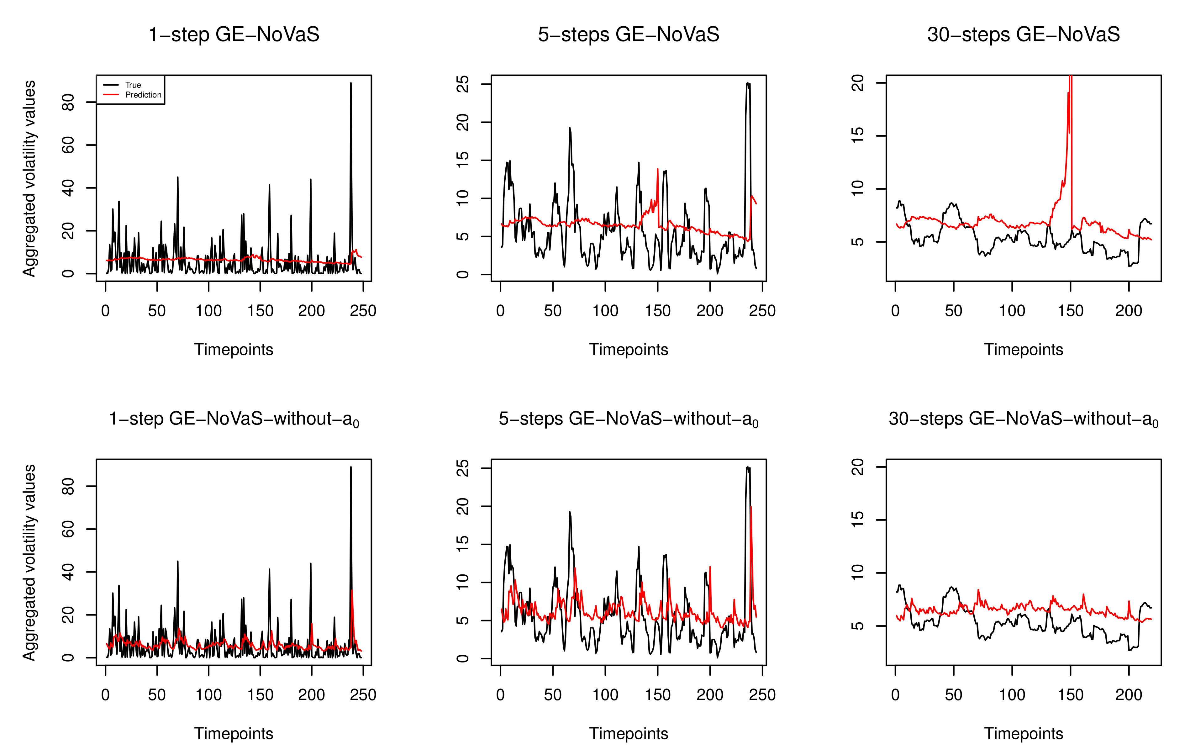
2.3. The Potential Instability of the GE-NoVaS Method

Next, we provide an illustration to compare the GE-NoVaS and GE-NoVaS-without-${\tilde{a}}_0$ methods in predicting the volatility of the Microsoft Corporation (MSFT) daily closing price from 8 January 1998 to 31 December 1999 and show an interesting finding that the long-term time-aggregated predictions of the GE-NoVaS method are unstable under the $L_2$ criterion. Based on the finding of Awartani and Corradi [14], squared log-returns can be used as a proxy for volatility to render a correct ranking of different GARCH models in terms of a quadratic loss function. Log-return series $\left\{Y_t\right\}$ can be computed by the equation shown below:

$$Y_t=100\times log(X_{t+1}/X_t)$$

(13)

where $\left\{X_t\right\}$ is the corresponding MSFT daily closing price series. For achieving a comprehensive comparison, we use 250 financial log-returns as a sliding window to perform POOS 1-step, 5-step and 30-step (long-term) ahead time-aggregated predictions under the $L_2$ criterion. Then, we roll this window through the whole dataset, i.e., we use $\{Y_1,\cdots ,Y_{250}\}$ to predict $Y_{251}^2,\{Y_{251}^2,\cdots ,Y_{255}^2\}$ and $\{Y_{251}^2,\cdots ,Y_{280}^2\}$; then, we use $\{Y_2,\cdots ,Y_{251}\}$ to predict $Y_{252}^2,\{Y_{252}^2,\cdots ,Y_{256}^2\}$ and $\{Y_{252}^2,\cdots ,Y_{281}^2\}$, for 1-step, 5-step and 30-step aggregated predictions, respectively, and so on. We can define all 1-step, 5-step and 30-step-ahead time-aggregated predictions as $\left\{{\widehat{Y}}_{k,1}^2\right\}$, $\left\{{\widehat{Y}}_{i,5}^2\right\}$ and $\left\{{\widehat{Y}}_{j,30}^2\right\}$, which are presented as below:

$$\begin{array}{cc}\hfill & \mathrm{Assume}\mathrm{that}\mathrm{there}\mathrm{are}\mathrm{a}\mathrm{total}\mathrm{of}N\log -\mathrm{return}\mathrm{data}\mathrm{points}:\hfill \\ \hfill & {\widehat{Y}}_{k,1}^2={\widehat{Y}}_{k+1}^2,k=250,251,\cdots ,N-1\hfill \\ \hfill & {\widehat{Y}}_{i,5}^2=\sum _{m=1}^5{\widehat{Y}}_{i+m}^2,i=250,251,\cdots ,N-5\hfill \\ \hfill & {\widehat{Y}}_{j,30}^2=\sum _{m=1}^{30}{\widehat{Y}}_{j+m}^2,j=250,251,\cdots ,N-30\hfill \end{array}$$

(14)

In Equation (14), ${\widehat{Y}}_{k+1}^2,{\widehat{Y}}_{i+m}^2,{\widehat{Y}}_{j+m}^2$ are single-step predictions of squared log-returns by the two NoVaS-type methods. To obtain the “Prediction Errors” for the two methods, we can calculate the “loss” by comparing the aggregated prediction results with the realized aggregated values based on Equation (15):

$$L_{p,h}=\sum _p{({\widehat{Y}}_{p,h}^2-\sum _{m=1}^h\left(Y_{p+m}^2\right))}^2,p\in \{k,i,j\};h\in \{1,5,30\}$$

(15)

where $\left\{Y_{p+m}^2\right\}$ are realized squared log-returns. To show the potential instability of the GE-NoVaS method under the $L_2$ criterion, we take $\alpha$ to be 0.5 to build a toy example. In the algorithm when performing the GE-NoVaS method, $\alpha$ could take an optimal value from a discrete set $\{0.1,\cdots ,0.8\}$ based on the prediction performance.

From Figure 1, we can clearly see that the GE-NoVaS-without-${\tilde{a}}_0$ method can better capture different steps’ true time-aggregated features. On the other hand, the GE-NoVaS method returns unstable results for 30-step-ahead time-aggregated predictions. Besides, we can see that the 1-step-ahead POOS prediction returned by the GE-NoVaS method is almost a flat curve, which is actually meaningless. Similarly, for the 5-step-ahead time-aggregated prediction case, the POOS prediction of the GE-NoVaS method fails to match the true time-aggregated values.

3. Data Analysis and Results

To perform extensive data analysis in a bid to validate our method, we deploy POOS predictions using two NoVaS and standard GARCH(1,1) methods with simulated and real-world data. All results are collated in

Table 1. Comparisons of different methods’ forecasting performance.

		GE-NoVaS	GE-NoVaS-without-${\tilde{\mathit{a}}}_0$	GARCH(1,1)	p-Value(CW Test)
Simulated-1-year-data	Model-1-1step	0.91369	0.88781	1.00000
	Model-1-5steps	0.61001	0.52872	1.00000
	Model-1-30steps	0.77250	0.73604	1.00000
	Model-2-1step	0.97796	0.94635	1.00000
	Model-2-5steps	0.98127	0.96361	1.00000
	Model-2-30steps	1.38353	0.98872	1.00000
	Model-3-1step	0.99183	0.92829	1.00000
	Model-3-5steps	0.77088	0.67482	1.00000
	Model-3-30steps	0.79672	0.71003	1.00000
	Model-4-1step	0.83631	0.78087	1.00000
	Model-4-5steps	0.38296	0.34396	1.00000
	Model-4-30steps	0.00199	0.00201	1.00000
2-years-data	2018∼2019-MCD-1step	0.99631	0.99614	1.00000	0.00053
	2018∼2019-MCD-5steps	0.95403	0.92120	1.00000	0.03386
	2018∼2019-MCD-30steps	0.75730	0.62618	1.00000	0.19691
	2018∼2019-BAC-1step	0.98393	0.97966	1.00000	0.09568
	2018∼2019-BAC-5steps	0.98885	0.95124	1.00000	0.07437
	2018∼2019-BAC-30steps	1.14111	0.87414	1.00000	0.03643
1-year-data	2019-AAPL-1step	0.84533	0.80948	1.00000	0.25096
	2019-AAPL-5steps	0.85401	0.68191	1.00000	0.06387
	2019-AAPL-30steps	0.99043	0.73823	1.00000	0.17726
	2019-Djones-1step	0.96752	0.96365	1.00000	0.34514
	2019-Djones-5steps	0.98725	0.89542	1.00000	0.24529
	2019-Djones-30steps	0.86333	0.80304	1.00000	0.23766
	2019-SP500-1step	0.96978	0.92183	1.00000	0.45693
	2019-SP500-5steps	0.96704	0.75579	1.00000	0.24402
	2019-SP500-30steps	0.34389	0.29796	1.00000	0.08148
Volatile-1-year-data	11.2019∼10.2020-IBM-1step	0.80222	0.80744	1.00000	0.16568
	11.2019∼10.2020-IBM-5steps	0.38933	0.40743	1.00000	0.03664
	11.2019∼10.2020-IBM-30steps	0.01143	0.00918	1.00000	0.15364
	11.2019∼10.2020-CADJPY-1step	0.46940	0.48712	1.00000	0.16230
	11.2019∼10.2020-CADJPY-5steps	0.11678	0.13549	1.00000	0.06828
	11.2019∼10.2020-CADJPY-30steps	0.00584	0.00394	1.00000	0.15174
	11.2019∼10.2020-SP500-1step	0.97294	0.92349	1.00000	0.05536
	11.2019∼10.2020-SP500-5steps	0.96590	0.75183	1.00000	0.17380
	11.2019∼10.2020-SP500-30steps	0.34357	0.29793	1.00000	0.16022
	11.2019∼10.2020-Djones-1step	0.56357	0.57550	1.00000	0.11099
	11.2019∼10.2020-Djones-5steps	0.09810	0.11554	1.00000	0.45057
	11.2019∼10.2020-Djones-30steps	4.32 × ${10}^{-5}$	1.24 × ${\mathbf{10}}^{-\mathbf{5}}$	1.00000	0.68487

Note: The values presented in the GE-NoVaS and GE-NoVaS-without-${\tilde{a}}_0$ columns reflect the relative performance compared with the ‘standard’ GARCH(1,1) method. The null hypothesis of the CW test is that parsimonious and larger models have equal mean squared prediction error (MSPE). The alternative is that the larger model has a smaller MSPE.

. The optimal results for each data cases are highlighted in bold. For controlling the dependence of the prediction performance on the length of the dataset, we build datasets with two fixed lengths—250 or 500—to mimic 1-year or 2-year data, respectively. At the same time, we choose the window size for our rollover forecasting analysis to be 100 or 250 for the 1-year or 2-year datasets.

3.1. Simulation Study

We use the same simulation Models 1–4 from [4], shown below, to mimic four 1-year datasets. Recall that one NoVaS method can generate the $L_1$ or $L_2$ predictor and $\left\{W^{*}\right\}$ can be chosen from a normal distribution or empirical distribution; thus, there are four variants of one specific NoVaS method. We take the best-performing result among four variants of a specific NoVaS method to be its final prediction. Finally, we continue applying the formula in Equation (15) to measure the performance of the different methods, as described in Section 2.3.

• Model 1: Time-varying GARCH(1,1) with Gaussian errors
  $X_t={\sigma }_t{ϵ}_t,{\sigma }_t^2=0.00001+{\beta }_{1,t}{\sigma }_{t-1}^2+{\alpha }_{1,t}{X}_{t-1}^2,\left\{{ϵ}_t\right\}\sim i.i.d.N(0,1)$
  ${\alpha }_{1,t}=0.1-0.05t/n$; ${\beta }_{1,t}=0.73+0.2t/n,n=250$
• Model 2: Standard GARCH(1,1) with Gaussian errors
  $X_t={\sigma }_t{ϵ}_t,{\sigma }_t^2=0.00001+0.73{\sigma }_{t-1}^2+0.1X_{t-1}^2,\left\{{ϵ}_t\right\}\sim i.i.d.N(0,1)$
• Model 3: (Another) Standard GARCH(1,1) with Gaussian errors
  $X_t={\sigma }_t{ϵ}_t,{\sigma }_t^2=0.00001+0.8895{\sigma }_{t-1}^2+0.1X_{t-1}^2,\left\{{ϵ}_t\right\}\sim i.i.d.N(0,1)$
• Model 4: Standard GARCH(1,1) with Student-t errors
  $X_t={\sigma }_t{ϵ}_t,$${\sigma }_t^2=0.00001+0.73{\sigma }_{t-1}^2+0.1X_{t-1}^2,$
  $\left\{{ϵ}_t\right\}\sim i.i.d.t$$\mathrm{distribution}\mathrm{with}\mathrm{five}\mathrm{degrees}\mathrm{of}\mathrm{freedom}$

Result analysis: From the first block of Table 1, we can read that both NoVaS methods are superior to the GARCH(1,1) model. Although these simulated datasets are generated from GARCH(1,1)-type models, the GE-NoVaS-without-${\tilde{a}}_0$ method can bring around 66% and 48% improvements compared to the GARCH(1,1) model for 5-step-ahead time-aggregated predictions of Model-4 and Model-1 data, respectively. Notably, GARCH(1,1) brings poor results for the 30-step-ahead time-aggregated predictions of Model-4 simulated data, which implies that such a classical method is impaired by error accumulation problems when long-term predictions are required. On the other hand, the model-free NoVaS method can avoid this issue. Taking a closer look at these results, we can observe that almost all optimal results come from applying the GE-NoVaS-without-${\tilde{a}}_0$ method. Moreover, the GE-NoVaS method is surpassed by GARCH(1,1) when forecasting 30-step-ahead time-aggregated Model-2 data. On the other hand, the GE-NoVaS-without-${\tilde{a}}_0$ method provides consistently stable results. These results imply that the GE-NoVaS-without-${\tilde{a}}_0$ method dominates the GE-NoVaS method when predicting long-term or short-term time-aggregated predictions. Besides, using the same generated models from the previous study of the NoVaS method [4] ensures fairness. Additionally, with simulation implementations, the ability against model misspecification of NoVaS methods is verified in Appendix A.

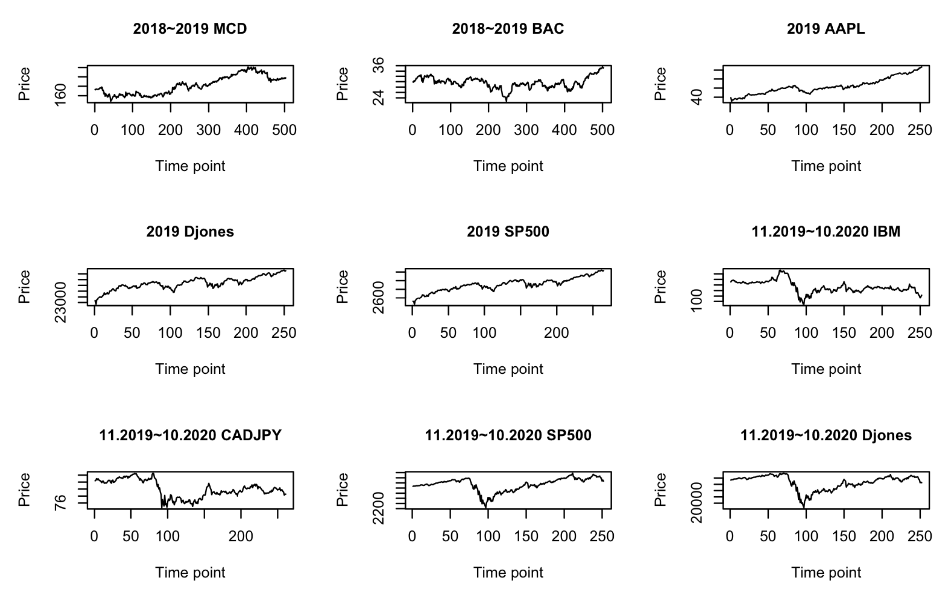
3.2. A Few Real Datasets

We also present a variety of real-world datasets of different size and intrinsic behavior:

• 2-year period data: 2018∼2019 stock price data.
• 1-year period data: 2019 stock price and index data.
• 1-year period volatile data due to pandemic: 11.2019∼10.2020 stock price, currency and index data.

Taking into account three types of real-world data is necessary to challenge our new method and explore the existing method in different regimes. We also tactically pay more attention to short and volatile data since this is a more challenging task to handle. Equation (13) is continually used to obtain the log-return series of different datasets.

Before comparing in depth the forecasting performance of the NoVaS-type and GARCH methods, we first investigate the properties of the used datasets. From Figure 2, we can see that there were huge variations in the four datasets during 11.2019∼10.2020, which implies the extreme fluctuations in global economics due to the COVID-19 pandemic. We wished to apply such datasets to test whether the NoVaS-type methods can achieve good forecasting performance for such volatile data.

Besides, it is natural to question whether these datasets are stationary. In a comprehensive manner, we choose three statistical tests—Augmented Dickey–Fuller (ADF) Test [15], Phillips–Perron (PP) Unit Root Test [16] and Kwiatkowski–Phillips–Schmidt–Shin (KPSS) Test [17]—to check the stationarity of the squared log-returns series of each selected dataset. One aspect that should be noticed is that the number of lags is crucial for the ADF test. If the included lag is too small, then the remaining serial correlation in the errors will bias the test. If this number is larger, the power of the test will suffer. Here, we consider taking the longest lag that is statistically significant. More specifically, we determine this longest lag by observing the last lag that crosses through the confidence interval lines of the autocorrelation plot. Besides, we apply a long version of the truncation lag parameter on both the PP and KPSS tests. The results of the three tests are tabulated in

Table A4. p-values of three stationarity tests.

	ADF	KPSS	PP
2018∼2019 MCD	0.01	0.10	0.01
2018∼2019 BAC	0.01	0.10	0.01
2019 AAPL	0.01	0.10	0.01
2019 Djones	0.10	0.10	0.01
2019 SP500	0.18	0.10	0.01
11.2019∼10.2020 IBM	0.31	0.05	0.01
11.2019∼10.2020 CADJPY	0.01	0.10	0.01
11.2019∼10.2020 SP500	0.23	0.08	0.01
11.2019∼10.2020 Djones	0.22	0.08	0.01

Note: The null hypothesis of the ADF and PP tests is that the tested series is non-stationary. Therefore, if the ADF and PP tests are rejected, it means that this tested series is stationary. On the other hand, the null hypothesis of KPSS is that the series is stationary.

. Combining these results, we can argue that most of the squared log-return series in the normal time period are stationary. However, during the volatile time period, the squared log-returns of IBM, SP500 and Dow Jones are thought to be non-stationary by the ADF test. The KPSS test also returns small p-values for these three datasets. These results are consistent with our conjecture that data tend to show non-stationarity during volatile periods. Again, it will be interesting to see if the NoVaS-type methods can offer good forecasting performance for non-stationary data. Recall that Chen and Politis [3] found that the NoVaS methodology generally outperforms the GARCH benchmark on the one-step-ahead point prediction of non-stationary data (involving local stationarity and/or structural breaks). However, they only considered two real-world time series. Here, we extend such empirical study to short- and long-term time-aggregated predictions with sufficient data examples.

• Remark (One ARCH-type model for non-stationary data): Since our stationarity tests suggest that some series may not be stationary, we can consider applying ARCH-without-intercept, which is a variant of the ARCH model. This variant is non-stationary but stable in the sense that the observed process has non-degenerated distribution. Moreover, it appears to be an alternative to common stationary but highly persistent GARCH models [18]. Inspired by this ARCH-type model, the NoVaS method may be further improved by removing the corresponding intercept term $\alpha s_{t-1}^2$ in Equations (1) and (6). More empirical experiments could be conducted along this direction.
• Result analysis: From the last three blocks of Table 1, there is no optimal result that comes from the GARCH(1,1) method. When the target data are short and volatile, GARCH(1,1) gives poor results for 30-step-ahead time-aggregated predictions, such as the volatile Djones, CADJPY and IBM cases. Among the two NoVaS methods, the GE-NoVaS-without-${\tilde{a}}_0$ method outperforms the GE-NoVaS method for the three types of real-world data. More specifically, around 70% and 30% improvements are created by our new method compared to the existing GE-NoVaS method when forecasting 30-step-ahead time-aggregated volatile Djones and CADJPY data, respectively. We should also notice that the GE-NoVaS method is again surpassed by the GARCH(1,1) model on 30-step-ahead aggregated predictions of 2018∼2019 BAC data. On the other hand, the GE-NoVaS-without-${\tilde{a}}_0$ method performs stably. These comprehensive prediction comparisons cover the shortage of empirical analyses of NoVaS methods, and imply that NoVaS-type methods are indeed valid and efficient for real-world short- or long-term predictions of three main types of econometric data. See Appendix A for more results.

3.3. Statistical Significance

However, one may suggest that the victory of our new methods is only specific to these samples. Therefore, we challenge this superiority by testing the statistical significance. Noting that the GE-NoVaS-without-${\tilde{a}}_0$ method is a nested method (taking ${\tilde{a}}_0=0$ in the larger model) compared with the GE-NoVaS method, we deploy the CW test [19] to ensure that the removing-${\tilde{a}}_0$ idea is also statistically reasonable; see the p-value column in Table 1 for the tests’ results. The reason for not performing CW tests on the simulation cases is that the prediction performance of each simulation is the average value of 5 replications. These CW test results imply that the null hypothesis should not be rejected for almost all cases under a 5% level of significance, which confirms the equivalence of the new method to the existing one.

4. Summary

In previous studies of NoVaS methods, only a few real-word data analyses were performed [2,3,4]. Here, we provide extensive data analyses to address the lack of real-world data experiments. Our results are consistent with previous findings and substantiate the effectiveness of the NoVaS method again, i.e., the NoVaS method is more efficient and stable than the classical GARCH method for short-term predictions. Further, we reveal the ability of NoVaS-type methods to perform long-term time-aggregated forecasting. Beyond this, we propose a new NoVaS method that outperforms the state-of-the-art GE-NoVaS method. Our findings in this article are summarized as follows:

• Existing GE-NoVaS and new GE-NoVaS-without-${\tilde{a}}_0$ methods provide substantial improvements for time-aggregated prediction, which hints towards the stability of NoVaS-type methods for providing long-horizon inferences.
• Our new method has superior performance to the GE-NoVaS method, especially for shorter sample sizes or more volatile data. This is significant given that GARCH-type models are difficult to estimate in shorter samples.
• We provide a statistical hypothesis test that shows that our model provides a more parsimonious fit, especially for long-term time-aggregated predictions.

5. Discussion

In this article, we explored the GE-NoVaS method toward short and long time-aggregated predictions and proposed a new variant that is based on a parsimonious model, has better empirical performance and yet is statistically reasonable. Although our new method is in a parsimonious form, it still obeys the autoregressive prediction rule and it is more stable for performing predictions under $L_2$ risk criterion than current the GE-NoVaS method. We should note that the unknown coefficients of both the GE-NoVaS (${\tilde{a}}_0,a_1,\cdots ,a_p$) and GE-NoVaS-without-${\tilde{a}}_0$ ($a_1,\cdots ,a_p$) methods are in exponential form, which implies that the correlations within series data are decreasing in exponential speed with the increasing time order. However, this specific form is not suitable for use for predicting all datasets. In other words, we anticipate performing NoVaS prediction without fixing the unknown coefficients in an invariant form to satisfy the variety of real-world econometric datasets. Therefore, building a NoVaS method with a more arbitrary coefficient form can be a future research direction. In addition, we should also note that there is a high demand to perform efficient forecasting for integer time series data. For example, a relevant topic regarding such integer-value prediction is forecasting COVID-19 cases. It will be beneficial to develop a variant of NoVaS for integer-value data. Moreover, in the financial market, the stock data move together. Thus, it would be exciting to see if one can perform model-free predictions in a multiple time series scenario. We hope that this article will open up avenues where one can explore other specific transformation structures to improve the existing forecasting frameworks and aid in specific tasks.

From a statistical inference point of view, one can also construct prediction intervals for these predictions using bootstrap. Such prediction intervals are well sought after in the econometrics literature and some results on the asymptotic validity of these can be provided. Additionally, we can also explore dividing the dataset into test and training in some optimal way and see if this can improve the performance of these methods.

In addition, there are some model-free methods based on machine learning to perform prediction tasks. These modern techniques enjoy high accuracy, but are time-consuming and lack of statistical inference. On the other hand, our new method and existing NoVaS methods are time-efficient and outperform classical GARCH-type methods significantly. More importantly, NoVaS-type methods can provide concrete statistical inference. Thus, it will be interesting to challenge NoVaS-type methods’ forecasting accuracy with machine-learning-based methods.

References

1. Politis, D.N. A Normalizing and Variance-Stabilizing Transformation for Financial Time Series; Elsevier Inc.: Amsterdam, The Netherlands, 2003. [Google Scholar]
2. Gulay, E.; Emec, H. Comparison of forecasting performances: Does normalization and variance stabilization method beat GARCH (1, 1)-type models? Empirical evidence from the stock markets. J. Forecast. 2018, 37, 133–150. [Google Scholar] [CrossRef]
3. Chen, J.; Politis, D.N. Time-varying NoVaS Versus GARCH: Point Prediction, Volatility Estimation and Prediction Intervals. J. Time Ser. Econom. 2020, 1. [Google Scholar] [CrossRef]
4. Chen, J.; Politis, D.N. Optimal multi-step-ahead prediction of ARCH/GARCH models and NoVaS transformation. Econometrics 2019, 7, 34. [Google Scholar] [CrossRef] [Green Version]
5. Chudỳ, M.; Karmakar, S.; Wu, W.B. Long-term prediction intervals of economic time series. Empir. Econ. 2020, 58, 191–222. [Google Scholar] [CrossRef] [Green Version]
6. Karmakar, S.; Chudy, M.; Wu, W.B. Long-term prediction intervals with many covariates. arXiv 2020, arXiv:2012.08223. [Google Scholar] [CrossRef]
7. Kitsul, Y.; Wright, J.H. The economics of options-implied inflation probability density functions. J. Financ. Econ. 2013, 110, 696–711. [Google Scholar] [CrossRef] [Green Version]
8. Bansal, R.; Kiku, D.; Yaron, A. Risks for the long run: Estimation with time aggregation. J. Monet. Econ. 2016, 82, 52–69. [Google Scholar] [CrossRef] [Green Version]
9. Starica, C. Is GARCH (1, 1) as Good a Model as the Accolades of the Nobel Prize Would Imply? University Library of Munich: Munich, Germany, 2003; SSRN 637322. [Google Scholar]
10. Fryzlewicz, P.; Sapatinas, T.; Rao, S.S. Normalized least-squares estimation in time-varying ARCH models. Ann. Stat. 2008, 36, 742–786. [Google Scholar] [CrossRef]
11. Politis, D.N. The Model-Free Prediction Principle. In Model-Free Prediction and Regression; Springer: Berlin/Heidelberg, Germany, 2015; pp. 13–30. [Google Scholar]
12. Engle, R.F. Autoregressive conditional heteroscedasticity with estimates of the variance of United Kingdom inflation. Econom. J. Econom. Soc. 1982, 50, 987–1007. [Google Scholar] [CrossRef]
13. Chen, J. Prediction in Time Series Models and Model-free Inference with a Specialization in Financial Return Data. Ph.D. Thesis, University of California, San Diego, CA, USA, 2018. [Google Scholar]
14. Awartani, B.M.; Corradi, V. Predicting the volatility of the S&P-500 stock index via GARCH models: The role of asymmetries. Int. J. Forecast. 2005, 21, 167–183. [Google Scholar]
15. Said, S.E.; Dickey, D.A. Testing for unit roots in autoregressive-moving average models of unknown order. Biometrika 1984, 71, 599–607. [Google Scholar] [CrossRef]
16. Perron, P. Trends and random walks in macroeconomic time series: Further evidence from a new approach. J. Econ. Dyn. Control 1988, 12, 297–332. [Google Scholar] [CrossRef]
17. Kwiatkowski, D.; Phillips, P.C.; Schmidt, P.; Shin, Y. Testing the null hypothesis of stationarity against the alternative of a unit root: How sure are we that economic time series have a unit root? J. Econom. 1992, 54, 159–178. [Google Scholar] [CrossRef]
18. Hafner, C.M.; Preminger, A. An ARCH model without intercept. Econ. Lett. 2015, 129, 13–17. [Google Scholar] [CrossRef]
19. Clark, T.E.; West, K.D. Approximately normal tests for equal predictive accuracy in nested models. J. Econom. 2007, 138, 291–311. [Google Scholar] [CrossRef] [Green Version]
Figure 1. Curves of the true and predicted time-aggregated squared log-returns from GE-NoVaS and GE-NoVaS-without- a ˜ 0 methods.
Forecasting 03 00055 g001
Figure 2. Price series of selected 9 datasets.
Forecasting 03 00055 g002