Bootstrapped Holt Method with Autoregressive Coefficients Based on Harmony Search Algorithm

Abstract

Exponential smoothing methods are one of the classical time series forecasting methods. It is well known that exponential smoothing methods are powerful forecasting methods. In these methods, exponential smoothing parameters are fixed on time, and they should be estimated with efficient optimization algorithms. According to the time series component, a suitable exponential smoothing method should be preferred. The Holt method can produce successful forecasting results for time series that have a trend. In this study, the Holt method is modified by using time-varying smoothing parameters instead of fixed on time. Smoothing parameters are obtained for each observation from first-order autoregressive models. The parameters of the autoregressive models are estimated by using a harmony search algorithm, and the forecasts are obtained with a subsampling bootstrap approach. The main contribution of the paper is to consider the time-varying smoothing parameters with autoregressive equations and use the bootstrap method in an exponential smoothing method. The real-world time series are used to show the forecasting performance of the proposed method.

1. Introduction

Exponential smoothing methods were published in the late 1950s [1,2,3], and they are known as some of the most successful forecasting methods in the literature. There are many exponential smoothing methods in the literature, such as the single exponential smoothing method, Holt method, Holt-Winters method, etc. Each exponential smoothing method is used in different situations. If data has no trend and no seasonality, a simple exponential smoothing method is used for forecasting. If data has a linear trend and no seasonality, the Holt method is used for forecasting. If data has both trend and seasonality, the Holt-Winters method is used for forecasting. In the coming years, the damped trend model was proposed by [4] if data has an over-trend. The reason why exponential smoothing methods are popular in the literature is that the forecasting success of exponential smoothing methods is superior to complicated approaches such as [5,6,7]. In addition to these methods, [8] proposed a simple modification of the exponential smoothing method named the ATA method, which is an effective and simple method to use compared with complex approaches in recent years.

Moreover, ref. [9,10] developed state-of-the-art guidelines for the application of the exponential smoothing methodology. Ref. [11] proposed a uniformly-sampled-autoregressive-moving-average model for a second-order linear stochastic system. Ref. [12] introduced the optimal procedure of the Boolean Kalman filter over a finite horizon. Ref. [13] presented a general benchmarking framework applicable to computational intelligence algorithms for solving forecasting problems. Ref. [14] proposed a new enhanced optimization model based on the bagged echo state network and improved by a differential evolution algorithm to estimate energy consumption. Ref. [15] introduced a two-stage Bayesian optimization framework for scalable and efficient inference in state-space models.

The method proposed by [2] is one of the effective exponential smoothing methods for forecasting data with trend. The Holt method has a forecasting equation and two smoothing equations, which are for the level of the series and slope of the trend as given in Equations (1)–(3).

$${\widehat{x}}_{n+1}={\widehat{l}}_n+{\widehat{b}}_n$$

(1)

$${\widehat{l}}_n={\lambda }_1{x}_n+\left(1-{\lambda }_1\right)x_n$$

(2)

$${\widehat{b}}_n={\lambda }_2\left({\widehat{l}}_n-{\widehat{l}}_{n-1}\right)+\left(1-{\lambda }_2\right){\widehat{b}}_{n-1}$$

(3)

In Equations (1)–(3), ${\lambda }_1$ and ${\lambda }_2$ are the smoothing parameters of mean level and slope, respectively, and these parameters get values between zero and one. In these equations, the initial values are obtained by applying simple linear regression to the series. In addition, in these equations, trend and level update formulas are only based on a lag.

In this study, the Holt method is modified by using time-varying smoothing parameters instead of fixed on time, and the smoothing parameters of mean level and slope are obtained for each observation with first-order autoregressive models. The parameters of the autoregressive models are estimated by using the harmony search algorithm (HSA). With these contributions, the proposed method eliminates the initial parameter determination problem. Moreover, the forecasts for the proposed method are obtained from sampling distributions of forecasts.

The proposed method is applied to Istanbul Stock Exchange data sets between the years 2000 and 2017 with different test lengths. The obtained results are compared with many methods in the literature. The brief information for HSA is given in Section 2. The proposed method is introduced, and the implementation results are given in Section 3 and Section 4 respectively. The final section is for conclusion and discussion.

2. Harmony Search Algorithm

HSA algorithm was proposed by [16]. HSA is a heuristic algorithm that simulates the notes of musicians. The principle of HSA is that the musicians in an orchestra play the best melody harmonically with the notes they play. Just as a chromosome in the genetic algorithm or a particle in particle swarm optimization represents a solution, a harmony in a harmony memory represents a solution in the harmony search algorithm. In HSA, each musician has a decision variable and each note in the memory of each musician corresponds to a different solution of that decision variable. Each harmony consists of different notes and each note corresponds to the decision variable. HSA aims to investigate whether the obtained solution vector is better than the worst solution in memory. The HSA is given below in steps in Algorithm 1.

Algorithm 1 The algorithm of HSA

Step 1. Determination of parameters to be used in HSA:

• XHM: Harmony memory;

• HMS: Harmony memory search;

• HMCR: Harmony memory considering rate;

• PAR: Pitch adjusting rate;

• n: the number of variables.

Step 2. Creating of the harmony memory.

HM for HSA is generated as in Equation (4). $$HM=\left[\begin{array}{cccc}{x}_{11}& x_{12}& \cdots & x_{1n}\\ x_{21}& x_{22}& \cdots & x_{2n}\\ ⋮& ⋮& ⋮& ⋮\\ x_{HMS1}& x_{HMS2}& x_{HMS3}& x_{HMSn}\end{array}\right]=\left[\begin{array}{c}{x}_1^{\prime }\\ x_2^{\prime }\\ \\ x_{HMS}^{\prime }\end{array}\right]$$ (4)

Here, $x_{ij},i=1,2,\dots HMS ;j=1,2,\cdots ,n$ is expressed as a note value and is generated randomly.

In HSA, each solution vector is denoted by $x_i^{\prime },i=1,2,\cdots ,HMS$. In HSA, there are HMS solution vectors. The representation of the first solution vector is given in Equation (5). $$x_1^{\prime }=\left[x_{11},x_{12},\cdots ,x_{1n}\right]$$ (5)

Step 3. Calculation of objective function values.

The objective function values are calculated for each solution vector generated randomly as given in Equation (6). $$\left[\begin{array}{cccc}{x}_{11}& x_{12}& \cdots & x_{1n}\\ x_{21}& x_{22}& \cdots & x_{2n}\\ ⋮& ⋮& ⋮& ⋮\\ x_{HMS1}& x_{HMS2}& x_{HMS3}& x_{HMSn}\end{array}\right]=\left[\begin{array}{c}{x}_1^{\prime }\\ x_2^{\prime }\\ \\ x_{HMS}^{\prime }\end{array}\right]=\left[\begin{array}{c}f\left(x_1^{\prime }\right)\\ f\left(x_2^{\prime }\right)\\ ⋮\\ f\left(x_{HMS}^{\prime }\right)\end{array}\right]$$ (6)

Step 4. Improvement of a new harmony.

While the probability of $HMCR$ with a value between 0 and 1 is to select a value from the existing values in the HM, (1-HMCR) value is the ratio of a random value selected from the possible value ranges. The new harmony is obtained with the help of Equation (7). $$x_{ijnew}=\left\{\begin{array}{cc}\hspace{1em}{x}_{ijnew}\in \left\{x_{ij};\mathrm{i}=1,,2,\cdots ,\mathrm{HMS}\right\}\hfill & \mathrm{if}\mathrm{rnd}<\mathrm{HMCR}\\ x_{ijnew}\in \left\{\left[\min (x_{ij}),\max (x_{ij})\right]; i=1,2, \dots HMS\right\}& \mathrm{otherwise}\end{array}\right.$$ (7)

It is decided by the $PAR$ parameter whether the toning process can be applied to each selected decision variable with the possibility of $HMCR$ or not as given in Equation (8). $$x_{ijnewpitch}=\left\{\begin{array}{cc}Yes\hfill & rnd<PAR\hfill \\ No\hfill & otherwise\hfill \end{array}\right.$$ (8)

In Equation (8), $rnd$ is generated randomly between $U\left(0,1\right)$. If this random number is smaller than the $PAR$ value, this value is changed to the closest value to it. If the tonalization will be made for each $x_{ijnew}$ decision variable and the value of $x_{ijnew}$ is assumed to be the $k\mathrm{th}$ value within the vector of the value variable, the new value of $x_{ijnew}\left(k\right)$ is $x_{ij}\leftarrow x_{ij}\left(k+m\right)$, and $m\in \left\{\cdots ,-2,-1,1,2,\cdots \right\}$ is the neighboring index.

Step 5. Updating the harmony memory.

If the new harmony vector is better than the worst vector in the $HM$, the worst vector is removed from the memory, and the new harmony vector is included in the HM instead of the removed vector.

Step 6. Stop condition check.

Steps 4–6 are repeated until the termination criteria are met. Possible values for HMCR and PAR in literature are between 0.7–0.95 and 0.05–0.7, respectively [17].

3. Proposed Method

Although the Holt method is used as an efficient forecasting method, it has many problems that are obvious and need to be resolved. The first of these problems is the determination of initial trend and level values. The second problem of the Holt method is that the trend and level update formulas are only based on a lag. To avoid these problems and increase the forecasting performance of the Holt method, the advantages and innovations of the proposed method are given step by step as below:

• The smoothing parameters are varied from observation to observation using first-order autoregressive equations;
• The optimal parameters of the Holt method are determined with HSA;
• The forecasts are obtained by the Sub-sampling Bootstrap method.

The algorithm of the proposed method is also given in Algorithm 2.

Algorithm 2 The algorithm of the proposed method

Step 1. Determine the parameters of the training process:

• # observation of test set: $ntest$;

• HMS;

• HMCR;

• PAR;

• # bootstrap samples: nbst;

• bootstrap sample size: bss.

Step 2. Select bootstrap samples from the training set randomly.

Steps from 2.1. to 2.2 are repeated $nbst$ times. $x_{t,j}^{*}$ presents $j\mathrm{th}$ bootstrap time series.

Step 2.1. Select a starting point of the block $\left(spb\right)$ as an integer from a discrete uniform distribution with parameters $[1,ntrain$-bss+1$]$.

Step 2.2. Create bootstrap time series as given in Equation (9). $$x_{t,j}^{*}=\left\{x_{spb},x_{spb+1},\dots ,x_{spb+bss-1}\right\}, j=1,2,\dots nbst$$ (9)

Step 3. Apply regression analysis to determine the initial bounds for level $\left(L\left(0\right)\right)$ and trend $\left(B\left(0\right)\right)$ parameters by using $x_{t,j}^{*}$ bootstrap time series as the training set by using Equations (10)–(12). $$X={\left[1 1 \cdots 1;1 2 \cdots bss\right]}^{\prime }{}_{bss\ast 2}$$ (10) $$Y=x_{t,j}^{\ast }=\left[x_{spb},x_{spb+1},\dots ,x_{spb+bss-1}\right]\prime$$ (11) $$\widehat{\beta }=\left[\begin{array}{c}{\widehat{\beta }}_0\\ {\widehat{\beta }}_1\end{array}\right]={\left(X\prime X\right)}^{-1}X\prime Y$$ (12)

$(L\left(0\right)\in \left[{\widehat{\beta }}_0/2,2{\widehat{\beta }}_0\right])$ and trend $(B\left(0\right)\in \left[{\widehat{\beta }}_1/2,2{\widehat{\beta }}_1\right])$

Step 4. HSA is used to obtain the optimal parameters of the Holt method with autoregressive coefficients for each bootstrap time series. Steps 4.1 and 4.4 are repeated for each bootstrap time series.

Step 4.1. Generate the initial positions of HSA. The positions of harmony are $L\left(0\right), B\left(0\right),{\lambda }_1\left(0\right),{\lambda }_2\left(0\right),{\varphi }_{11},{\varphi }_{12},{\varphi }_{21} and {\varphi }_{22}$.

$L\left(0\right)$ and $B\left(0\right)$ are generated from $U\left(\widehat{{\beta }_0}/2,2\widehat{{\beta }_0}\right) and U\left(\widehat{{\beta }_1}/2,2\widehat{{\beta }_1}\right)$, respectively. ${\lambda }_1\left(0\right)$, ${\lambda }_2\left(0\right),{\varphi }_{11}$ and ${\varphi }_{21}$ are generated from $U\left(0,1\right)$. ${\varphi }_{12}$ and ${\varphi }_{22}$ are generated from $U\left(-1,1\right)$. The creation of the harmony memory for the proposed method is given in Equation (13), and the parameters that correspond to $k\mathrm{th}$ harmony are given in Table 1. The parameters corresponding to kth harmony. ${\mathit{x}}_1{}^{\mathit{k}}$ ${\mathit{x}}_2{}^{\mathit{k}}$ ${\mathit{x}}_3{}^{\mathit{k}}$ ${\mathit{x}}_4{}^{\mathit{k}}$ ${\mathit{x}}_5{}^{\mathit{k}}$ ${\mathit{x}}_6{}^{\mathit{k}}$ ${\mathit{x}}_7{}^{\mathit{k}}$ ${\mathit{x}}_8{}^{\mathit{k}}$ $L\left(0\right)$ $B\left(0\right)$ ${\lambda }_1\left(0\right)$ ${\lambda }_2\left(0\right)$ ${\varphi }_{11}$ ${\varphi }_{12}$ ${\varphi }_{21}$ ${\varphi }_{22}$ . $$HM=\left[\begin{array}{ccccc}{x}_1{}^1& x_2{}^1& x_3{}^1& \cdots & x_8{}^1\\ x_1{}^2& x_2{}^2& x_3{}^2& \cdots & x_8{}^2\\ ⋮& ⋮& ⋮& ⋮& ⋮\\ x_1{}^{HMS}& x_2{}^{HMS}& x_3{}^{HMS}& \cdots & x_8{}^{HMS}\end{array}\right]$$ (13)

Step 4.2. According to the initial positions of each harmony, fitness functions are calculated. The root of mean square error (RMSE) is preferred to use as a fitness function and is calculated as given in Equation (14). $$f_i=RMS{E}_i=\sqrt{\frac{1}{bss}{\displaystyle \sum }_{t=1}^{bss}{\left(x_{t,j}^{*}-{\widehat{x}}_{t,j}^{\ast }\right)}^2}, i=1,2,\dots ,HMS$$ (14)

In Equation (14), ${\widehat{x}}_{t,j}^{⁥}$ is the output for $j^{\mathrm{th}}$ bootstrap time series data and $k^{\mathrm{th}}$ harmony. ${\widehat{x}}_{t,j}^{*}$ is obtained by using Equations (15)–(19). $${\lambda }_1\left(t\right)={\varphi }_{11}+{\varphi }_{12}{\lambda }_1\left(t-1\right)$$ (15) $${\lambda }_2\left(t\right)={\varphi }_{21}+{\varphi }_{22}{\lambda }_2\left(t-1\right)$$ (16) $$L\left(t\right)={\lambda }_1\left(t\right)x_{t,j}^{*}+\left(1-{\lambda }_1\left(t\right)\right)\left(L\left(t-1\right)+B\left(t-1\right)\right)$$ (17) $$B\left(t\right)={\lambda }_2\left(t\right)\left(L\left(t\right)-L\left(t-1\right)\right)+\left(1-{\lambda }_2\left(t\right)\right)\left(B\left(t-1\right)\right)$$ (18) $${\widehat{x}}_{t+1,j}^{*}=L\left(t\right)+B\left(t\right)$$ (19)

Obtain RMSE values for each harmony, and save the best harmony which has the smallest RMSE.

Step 4.3. Improve new harmony.

$HMCR$ shows the probability that the value of a decision variable is selected from the current harmony memory. (1-$HMCR$) represents the random selection of the new decision variable from the existing solution space. $x_i^{\prime }$ shows the new harmony, obtained as in Equation (20). $$x_i^{\prime }=\left\{\begin{array}{cc}{x}_i^{\prime }\in \left\{x_i{}^1,x_i{}^2,\cdots , x_i{}^{HMS} \right\}& if \mathrm{rand}<HMCR\\ x_i^{\prime }\in X_{,}& otherwise\end{array}\right.$$ (20)

After this step, each decision variable is evaluated to determine whether a tonal adjustment is necessary. This is determined by the PAR parameter, which is the tone adjustment ratio. The new harmony vector is produced according to the randomly selected tones in the memory of harmony as given in Equation (21). Whether the variables are selected from the harmonic memory is determined by the HMCR ratio, which is between 0 and 1. $$x_i^{\prime }=\left\{\begin{array}{cc}{x}_i^{\prime }+rnd\left(0,1\right)*bw& if \mathrm{rnd}<\mathrm{PAR}\\ x_i^{\prime }& otherwise\end{array}\right.$$ (21)

$bw$ is a bandwidth selected randomly; $rnd$ (0; 1) represents a random number generated between 0 and 1.

Step 4.4. Harmony memory update.

In this step, the comparison between the newly created harmonies and the worst harmonies in the memory is made in terms of the values of the objective functions. If the newly created harmony vector is better than the worst harmony, the worst harmony vector is removed from the memory, and the new harmony vector is substituted for it.

Calculate RMSE values for $j^{th}$ bootstrap time series data and $k^{\mathrm{th}}$ harmony. Find the best harmony which has the minimum RMSE value for $j^{\mathrm{th}}$ bootstrap time series data.

Step 5. Calculate the forecasts for test data by using the best harmony for each bootstrap sample and their statistics.

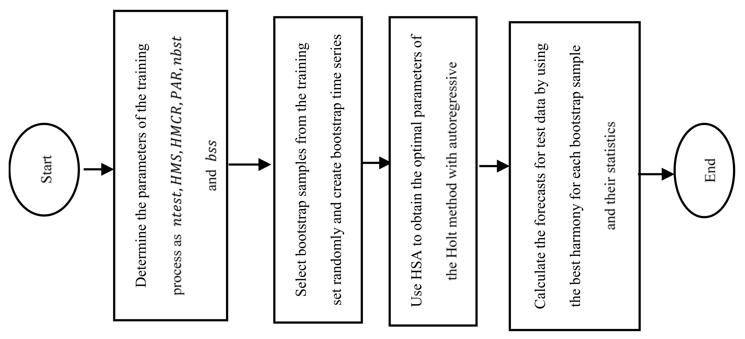
The obtained forecasts from the updated Equations for $j^{\mathrm{th}}$ bootstrap time series at $t$ time is represented by $F_t^i$. Forecasts and their statistics are calculated just as in Table 2. Forecasts for bootstrap samples. Time $\left(\mathit{t}\right)$/Bootstrap Sample $1$ $2$ $\dots$ $\mathit{n}\mathit{b}\mathit{s}\mathit{t}$ Median Standard Deviation 1 $F_1^1$ $F_1^2$ $\dots$ $F_1^{nbst}$ ${\widehat{F}}_1$ SE $({\widehat{F}}_1)$ 2 $F_2^1$ $F_2^2$ $\dots$ $F_2^{nbst}$ ${\widehat{F}}_2$ SE $({\widehat{F}}_2)$ $⋮$ $⋮$ $⋮$ $\dots$ $⋮$ $⋮$ $⋮$ ntest $F_{ntest}^1$ $F_{ntest}^2$ $\dots$ $F_{ntest}^{nbst}$ ${\widehat{F}}_{ntest}$ SE $({\widehat{F}}_{ntest})$ . In addition, the flowchart of the proposed method is given in Figure 1.

4. Applications

To evaluate the performance of the proposed method, the proposed method is applied to the Istanbul Stock Exchange (BIST) data sets observed daily between the years 2000 and 2017 with different test lengths as 10 and 20. To evaluate the performance of the proposed method, the proposed method is compared with the ATA method proposed by [8], Holt method, fuzzy regression functions approach (FF) proposed by [18], random walk (RW), multilayer perceptron artificial neural networks (MLP-ANN) and adaptive neural-fuzzy inference systems (ANFIS) method proposed by [19]. For a fair comparison of the methods, we used both statistical and computational intelligence forecasting methods. While the random walk was used as a simple forecasting method, the Holt and ATA methods were used as statistical forecasting methods. Moreover, MLP-ANN, ANFIS, and FF methods were used as computational intelligence forecasting methods. In the analysis process, the number of bootstrap samples and the bootstrap sample size is given as 100 for each data set. The RMSE and MAPE criteria were used for the comparison of the methods. The mean absolute percentage error (MAPE) is one of the most widely used measures of forecast accuracy, due to its advantages of scale-independency and interpretability [20]. The use of RMSE is very common, and it is considered an excellent general-purpose error metric for numerical predictions [21].

Table 3. All analysis results for each data set for RMSE criterion when the length of the test set is 10.

Data	ATA	Holt	FF	RW	MLP-ANN	ANFIS	PP
BIST2000	279.79	296.17	310.42	286.15	343.9	619.21	278.82
BIST2001	204.84	237.69	272.31	206.5	1106.89	710.82	189.75
BIST2002	325.08	319.78	357	331.87	620.78	399.13	332.13
BIST2003	354.79	355.55	380.82	349.79	1859.21	420.75	328.25
BIST2004	315.62	315.79	390.15	325.69	1807.8	641.43	313.7
BIST2005	316.75	315.36	328.84	342.69	2071.98	559.2	304.98
BIST2006	354.03	348.58	352.07	356.81	423.98	389.3	346.98
BIST2007	768.29	734.55	673.14	734.14	897.02	550.97	728.92
BIST2008	283.99	277.2	256.98	253.67	444.74	340.41	260.52
BIST2009	505.05	483.8	558.06	551.97	3117.96	736.78	473.4
BIST2010	577.68	594.9	583.52	591.88	725.15	588.36	576.4
BIST2011	697.64	710.04	849.68	726.5	1733.88	1037.87	737.83
BIST2012	355.5	350.46	368.26	358.17	3237.45	406.68	358.15
BIST2013	1905.64	1898.61	2105.05	1922.14	4369.35	2104.39	1871.45
BIST2014	1068.36	1025.18	1177.56	1059.97	2631.25	1435.01	1036.6
BIST2015	772.84	767.71	758.89	779.07	1080.69	714.69	751.41
BIST2016	431.86	433.52	450.67	434.01	520.1	424.34	652.25
BIST2017	861.26	869.23	1113.74	911.21	3777.62	1283.75	827.15

gives the all-analysis results for each data set for the RMSE criterion when the length of the test set is 10.

In Table 3, the proposed method has 59% success compared with the other methods in terms of the RMSE criterion when the test set is 10. To see the actual comparison results of the proposed method with other methods, we compare the rank values of each method and obtain the average rank values. For this purpose, we rank each method according to their success status for each time series analyzed. In such a ranking, the method with the lowest RMSE value will be named as the best method, and the rank value of it will be taken as 1. For this purpose, all methods were calculated according to rank order considering the RMSE criterion when the length of the test set is 10, and average rank values were obtained as in Figure 2.

From Figure 2, it is seen that the proposed method has a minimum average rank value compared with other methods, and the proposed method is the best method for RMSE criterion when the length of the test set is 10. In addition,

Table 4. All-analysis results for each data set for MAPE criterion when the length of the test set is 10.

Data	ATA	Holt	FF	RW	MLP-ANN	ANFIS	PP
BIST2000	0.0222	0.0233	0.0268	0.0236	0.0293	0.0507	0.0223
BIST2001	0.011	0.0124	0.0161	0.0112	0.0818	0.0506	0.0103
BIST2002	0.0253	0.0241	0.0267	0.0256	0.043	0.0287	0.0256
BIST2003	0.0163	0.0163	0.0178	0.0162	0.1008	0.0208	0.0154
BIST2004	0.0099	0.01	0.0129	0.0103	0.0735	0.0241	0.0099
BIST2005	0.0068	0.0069	0.0069	0.0074	0.0519	0.0126	0.0066
BIST2006	0.0068	0.0066	0.007	0.0067	0.0082	0.0076	0.0073
BIST2007	0.0098	0.01	0.0087	0.0095	0.0138	0.008	0.0095
BIST2008	0.0082	0.0075	0.0073	0.0071	0.0154	0.0093	0.0075
BIST2009	0.0067	0.0066	0.0077	0.0076	0.0595	0.0114	0.0071
BIST2010	0.006	0.0064	0.0058	0.0063	0.0085	0.0068	0.0061
BIST2011	0.0113	0.0116	0.0137	0.0118	0.0316	0.0165	0.0119
BIST2012	0.004	0.0039	0.004	0.0039	0.041	0.0042	0.004
BIST2013	0.022	0.0219	0.0254	0.0223	0.0608	0.0258	0.0216
BIST2014	0.0092	0.009	0.0101	0.0094	0.0304	0.0118	0.0089
BIST2015	0.0083	0.0082	0.0078	0.0082	0.0109	0.0087	0.0082
BIST2016	0.0049	0.0048	0.0047	0.0048	0.0051	0.0046	0.0062
BIST2017	0.0052	0.0053	0.0076	0.0058	0.0318	0.0092	0.0049

gives the all-analysis results for each data set for the MAPE criterion given in Equation (22) when the length of the test set is 10.

$$MAPE=\frac{1}{ntest}{\displaystyle \sum }_{t=1}^{ntest}\left|\frac{X_t-{\widehat{X}}_t}{X_t}\right|$$

(22)

In Table 4, the proposed method has 39% success compared with the other methods in terms of the MAPE criterion when the test set is 10. Looking at the rank evaluation results for the MAPE criterion when the test set length is 10 given in Figure 3, it is seen that the proposed method is in third place among all methods.

Table 5. All-analysis results for each data set for RMSE criterion when the length of the test set is 20.

Data	ATA	Holt	FF	RW	MLP-ANN	ANFIS	PP
BIST2000	680.61	680.33	713.87	682.74	2868.94	825.58	681.58
BIST2001	315.19	326.20	372.36	312.96	1030.82	540.36	296.32
BIST2002	388.51	389.17	390.47	393.48	392.16	432.21	383.70
BIST2003	313.25	339.08	456.83	311.18	2201.77	558.18	288.38
BIST2004	329.12	329.30	366.48	335.16	1479.79	554.62	319.35
BIST2005	426.84	415.74	496.57	433.66	2940.74	632.79	463.17
BIST2006	539.71	551.20	581.55	547.72	742.07	625.98	556.77
BIST2007	814.90	783.40	789.45	774.91	854.08	660.30	762.16
BIST2008	575.72	571.80	589.64	542.31	766.02	624.59	541.21
BIST2009	492.91	510.09	518.55	516.25	2794.96	623.04	492.17
BIST2010	867.04	921.85	885.97	850.14	1193.33	965.97	864.93
BIST2011	757.81	728.63	849.50	790.69	1141.08	772.13	774.14
BIST2012	592.96	564.85	605.32	544.81	5641.93	1224.80	517.44
BIST2013	1687.26	1680.69	1888.99	1709.07	2453.56	1821.80	1669.36
BIST2014	1318.63	1315.91	1323.78	1315.91	1936.51	1610.11	1318.91
BIST2015	1242.98	1263.71	1223.85	1225.07	2322.70	1189.75	1213.33
BIST2016	650.22	662.26	648.96	599.52	699.81	728.46	604.62
BIST2017	1010.73	1011.04	1165.70	1031.37	2981.64	1134.55	833.03

also gives the all-analysis results for each data set for the RMSE criterion when the length of the test set is 20. In Table 5, the proposed method has a 61% success rate. Considering the situations where the proposed method is not the best, it stands out as the second-best method in many time-series analyses. Moreover, the rank evaluation results for all methods for the RMSE criterion when the length of the test set is 20 are given in Figure 4. In addition,

Table 6. All-analysis results for each data set for MAPE criterion when the length of the test set is 20.

Data	ATA	Holt	FF	RW	MLP-ANN	ANFIS	PP
BIST2000	0.0540	0.0547	0.0615	0.0557	0.3091	0.0748	0.0546
BIST2001	0.0176	0.0182	0.0212	0.0175	0.0746	0.0355	0.0178
BIST2002	0.0261	0.0263	0.0275	0.0272	0.0260	0.0311	0.0269
BIST2003	0.0145	0.0147	0.0219	0.0146	0.1216	0.0242	0.0144
BIST2004	0.0104	0.0101	0.0121	0.0108	0.0587	0.0184	0.0107
BIST2005	0.0087	0.0082	0.0097	0.0091	0.0744	0.0134	0.0096
BIST2006	0.0098	0.0102	0.0109	0.0102	0.0143	0.0124	0.0105
BIST2007	0.0113	0.0108	0.0106	0.0104	0.0127	0.0095	0.0105
BIST2008	0.0180	0.0175	0.0193	0.0164	0.0223	0.0183	0.0167
BIST2009	0.0076	0.0079	0.0080	0.0080	0.0529	0.0097	0.0074
BIST2010	0.0101	0.0112	0.0103	0.0099	0.0129	0.0125	0.0100
BIST2011	0.0118	0.0110	0.0131	0.0124	0.0188	0.0117	0.0121
BIST2012	0.0063	0.0061	0.0064	0.0058	0.0728	0.0142	0.0056
BIST2013	0.0180	0.0179	0.0206	0.0182	0.0278	0.0202	0.0180
BIST2014	0.0121	0.0121	0.0122	0.0122	0.0203	0.0151	0.0120
BIST2015	0.0140	0.0145	0.0133	0.0135	0.0285	0.0129	0.0134
BIST2016	0.0065	0.0065	0.0059	0.0058	0.0068	0.0067	0.0058
BIST2017	0.0073	0.0073	0.0088	0.0077	0.0246	0.0087	0.0065

gives the all-analysis results for each data set for the MAPE criterion when the length of the test set is 20.

When the analysis results given in Table 6 are examined, even in the analyses in which the proposed method is not the best method, the proposed method often appears to be either the second-best or third-best method. We examine rank values to verify and highlight these results given in Figure 5.

Considering the average rank obtained from all methods, it can be said that the proposed method for the MAPE criterion has more successful results than other methods. As a final comment, when all analysis results are examined, it can be said from both average rank results and analysis results that the proposed method is a more successful method than other methods used in the comparison.

5. Conclusions and Discussion

Although the Holt method is used as a traditional time series forecasting method, it is known that it has some problems, such as the determination of the initial trend and level values and determining the trend and level update formulas. In this study, to overcome these problems, the parameters of the Holt method are optimized by using HSA, the smoothing parameters are varied by using first-order autoregressive equations, and the forecasting performance is improved by using the subsample bootstrap method.

When comparing the classical Holt method and the proposed method, it is clear that time-varying smoothing parameters and HSA provide important improvements in the forecasting results. The proposed method produces smaller RMSE values than the classical Holt method by about 70% in all analyses. If we compare the computation time of the proposed method with the classical Holt method, the proposed method needs more computation time because of using bootstrap and HSA algorithms, as expected. However, the computation time of the proposed method is very close to computational intelligence forecasting methods, and the computation time is not a problem for today’s personal computers. For the BIST series, the computation time is about three minutes.

In future studies, different artificial intelligence optimization techniques can be used to determine the optimal parameters of the Holt method, or the forecasts can be obtained by different bootstrap methods.

References

- Brown, R.G. Statistical Forecasting for Inventory Control; McGraw-Hill: New York, NY, USA, 1959. [Google Scholar]
- Holt, C.E. Forecasting Seasonals and Trends by Exponentially Weighted Averages (O.N.R. Memorandum No. 52); Carnegie Institute of Technology Pittsburgh: Pittsburgh, PA, USA, 1957. [Google Scholar]
- Winters, P.R. Forecasting sales by exponentially weighted moving averages. Manag. Sci. 1960, 6, 324–342. [Google Scholar] [CrossRef]
- Gardner, E.S., Jr.; McKenzie, E. Forecasting trends in time series. Manag. Sci. 1985, 31, 1237–1246. [Google Scholar] [CrossRef]
- Makridakis, S.G.; Fildes, R.; Hibon, M.; Parzen, E. The forecasting accuracy of major time series methods. J. R. Stat. Soc. Ser. D Stat. 1985, 34, 261–262. [Google Scholar]
- Makridakis, S.; Hibon, M. The M3-competition: Results, conclusions and implications. Int. J. Forecast. 2000, 16, 451–476. [Google Scholar] [CrossRef]
- Koning, A.J.; Franses, P.H.; Hibon, M.; Stekler, H.O. The M3 competition: Statistical tests of the results. Int. J. Forecast. 2005, 21, 397–409. [Google Scholar] [CrossRef]
- Yapar, G.; Selamlar, H.T.; Capar, S.; Yavuz, I. ATA method. Hacet. J. Math. Stat. 2019, 48, 1838–1844. [Google Scholar] [CrossRef]
- Gardner, E.S., Jr. Exponential smoothing. The state of the art. J. Forecast. 1985, 4, 1–28. [Google Scholar] [CrossRef]
- Gardner, E.S., Jr. Exponential smoothing: The state of the art—Part II. Int. J. Forecast. 2006, 22, 637–666. [Google Scholar] [CrossRef]
- Pandit, S.M.; Wu, S.M. Exponential smoothing as a special case of a linear stochastic system. Oper. Res. 1974, 22, 868–879. [Google Scholar] [CrossRef]
- Imani, M.; Braga-Neto, U.M. Optimal finite-horizon sensor selection for Boolean Kalman Filter. In Proceedings of the 2017 51st Asilomar Conference on Signals, Systems, and Computers, IEEE, Pacific Grove, CA, USA, 29 October–1 November 2017; pp. 1481–1485. [Google Scholar]
- Oprea, M. A general framework and guidelines for benchmarking computational intelligence algorithms applied to forecasting problems derived from an application domain-oriented survey. Appl. Soft Comput. 2020, 89, 106103. [Google Scholar] [CrossRef]
- Hu, H.; Wang, L.; Peng, L.; Zeng, Y.R. Effective energy consumption forecasting using enhanced bagged echo state network. Energy 2020, 193, 116778. [Google Scholar] [CrossRef]
- Imani, M.; Ghoreishi, S.F. Two-Stage Bayesian Optimization for Scalable Inference in State-Space Models. IEEE Trans. Neural Netw. Learn. Syst. 2021, 1–12. [Google Scholar] [CrossRef]
- Geem, Z.W.; Kim, J.H.; Loganathan, G.V. A new heuristic optimization algorithm: Harmony search. Simulation 2001, 76, 60–68. [Google Scholar] [CrossRef]
- Geem, Z.W. Optimal cost design of water distribution networks using harmony search. Eng. Optim. 2006, 38, 259–277. [Google Scholar] [CrossRef]
- Turkşen, I.B. Fuzzy functions with LSE. Appl. Soft Comput. 2008, 8, 1178–1188. [Google Scholar] [CrossRef]
- Jang, J.S. Anfis: Adaptive-network-based fuzzy inference system. IEEE Trans. Syst. Man Cybern. 1993, 23, 665–685. [Google Scholar] [CrossRef]
- Kim, S.; Kim, H. A new metric of absolute percentage error for intermittent demand forecasts. Int. J. Forecast. 2016, 32, 669–679. [Google Scholar] [CrossRef]
- Neill, S.P.; Hashemi, M.R. Ocean Modelling for Resource Characterization. Fundam. Ocean Renew. Energy 2018, 193–235. [Google Scholar] [CrossRef]