A Deep Learning Model for Forecasting Velocity Structures of the Loop Current System in the Gulf of Mexico

Abstract

Despite the large efforts made by the ocean modeling community, such as the GODAE (Global Ocean Data Assimilation Experiment), which started in 1997 and was renamed as OceanPredict in 2019, the prediction of ocean currents has remained a challenge until the present day—particularly in ocean regions that are characterized by rapid changes in their circulation due to changes in atmospheric forcing or due to the release of available potential energy through the development of instabilities. Ocean numerical models’ useful forecast window is no longer than two days over a given area with the best initialization possible. Predictions quickly diverge from the observational field throughout the water and become unreliable, despite the fact that they can simulate the observed dynamics through other variables such as temperature, salinity and sea surface height. Numerical methods such as harmonic analysis are used to predict both short- and long-term tidal currents with significant accuracy. However, they are limited to the areas where the tide was measured. In this study, a new approach to ocean current prediction based on deep learning is proposed. This method is evaluated on the measured energetic currents of the Gulf of Mexico circulation dominated by the Loop Current (LC) at multiple spatial and temporal scales. The approach taken herein consists of dividing the velocity tensor into planes perpendicular to each of the three Cartesian coordinate system directions. A Long Short-Term Memory Recurrent Neural Network, which is best suited to handling long-term dependencies in the data, was thus used to predict the evolution of the velocity field in each plane, along each of the three directions. The predicted tensors, made of the planes perpendicular to each Cartesian direction, revealed that the model’s prediction skills were best for the flow field in the planes perpendicular to the direction of prediction. Furthermore, the fusion of all three predicted tensors significantly increased the overall skills of the flow prediction over the individual model’s predictions. The useful forecast period of this new model was greater than 4 days with a root mean square error less than 0.05 cm·s${}^{-1}$ and a correlation coefficient of 0.6.

1. Introduction

Sustained large efforts in the ocean modeling community, such as the GODAE (Global Ocean Data Assimilation Experiment), which started in 1997 [1,2] and was renamed as OceanPredict in 2019 [3], have been made to promote and coordinate the approach to ocean forecasting among the international community. This large effort has seen many achievements in terms of predictive capabilities of ocean features temperature, salinity and sea surface height (SSH) and they are evaluated through a standard set of metrics [4]. However, the prediction of ocean currents has remained a challenge to this day—particularly in ocean regions that are characterized by rapid changes in their circulation due to changes in atmospheric forcing or due to the release of available potential energy through the development of dynamical instabilities. Predictions of ocean currents in the California current system can be found in [5], as well as other studies. This paper shows a correlation coefficient less than 0.3 after two days with a root mean square error (RMSE) of 7 cm·s${}^{-1}$ for the vertically integrated velocity component. Using mooring measurements in the same oceanographic region as that studied in Chao et al. [5], Shulman and Paduan [6] showed a significant decrease in the correlation coefficient and RMSE with depth between the observation and the model analyses while assimilating the 33 h filtered high-frequency (HF) radar surface current data. Ocean numerical models’ useful forecast window is no longer than two days over a given area with the best initialization possible, as shown by [7] in a dynamically active current system, such as the Loop Current (LC) in the Gulf of Mexico (GoM). The RMSE was 10 cm·s${}^{-1}$ and the correlation coefficient was 0.63 for the daily surface averaged predicted current. Ocean numerical model predictions quickly diverge from the observational field throughout the water and become unreliable, despite the fact that they can simulate the observed dynamics through other variables such as temperature, salinity and SSH. Numerical methods such as harmonic analysis are used to predict both short- and long-term tidal currents with significant accuracy. However, they are limited to the areas where the tide was measured.

Today’s full-water column predictions primarily rely on the use of finite-difference, finite-volume and finite-element methods to solve the primitive equation of motion in numerical models used to simulate ocean dynamics. The outputs of these models consist of the temporal prediction of three-dimensional fields of ocean state variables including both components of the horizontal velocity field, namely u and v along the x and y axes of the Cartesian coordinate system, respectively. In this study, we evaluate the application of a deep learning (DL—[8]) model to predict the three-dimensional velocity field from in-situ data. We demonstrate that the water column current velocity patterns can be learned by a DL model, which can then be used to predict the layered structure of the flow field. To this end, we show that the DL model is capable of accurately predicting the water column velocities more than four days in advance, doubling the current state of the art prediction window for in-situ currents. In this study, we propose a Recurrent Neural Network (RNN) Long Short-Term Memory (LSTM) model [9] to perform predictions of ocean currents’ speed and direction, as described in Section 2. LSTM networks have outperformed fully connected neural networks and other machine learning techniques in natural language processing [10,11] that has many similarities with ocean current predictions, as shown by Immas et al. [12]. RNNs have been the state-of-the-art method in modeling time series data for the last decade. In addition, this type of network has seen an increase in real-life applications, including but not limited to aquaculture [13], wind and solar energy resources management [14], bio science and medical applications [15] and also in industrial applications [16].

In a recent study by Wang et al. [17], an LSTM network was used to demonstrate the feasibility of medium-term (3 months) predictions of the GoM’s SSH in the LC region. The LSTM model was trained and tested with 18 years of analyzed daily SSH—“analyzed” indicates that the model calculated SSH was corrected with in-situ and remote sensing observations—from the Hybrid Coordinate Ocean Model (HYCOM)-GoM 1/25${}^{\circ }$ horizontal resolution [18]. The Loop Current (LC) and the mesoscale eddies associated with its nonlinear dynamics are the major drivers of the upper 1000 m water column circulation in the GoM [19]. The nonlinear dynamics of the LC is dominated by the shedding of anticyclonic eddies called Loop Current Eddies (LCE) at irregular time intervals [20,21,22]. The formation of the latter is primarily caused by the growth of baroclinic instability, which is associated with the formation of deep meanders and eddies [19,23,24]. Using metrics set in the literature for LC forecasting, the deep learning model predicted; overall, the LC system SSH frontal distance from reference points within 40 km nine weeks in advance. Furthermore, the model also predicted the final separation of two consecutive LC eddies through the SSH evolution, namely the eddies Cameron and Darwin 8 and 12 weeks in advance, respectively, an improvement over the 5–6-week useful forecast range of state of the art numerical models for the LC dynamics [25].

In this study, the LSTM model is applied to the prediction of water column velocity three-dimensional tensors. The prediction model is implemented on in-situ full water column current measurements collected in the LC region in the GoM between 2009 and 2011. Section 2 describes the measurements and their four-dimensional structure as well as the metrics used to assess the model’s skills. Section 3 presents the LTSM prediction model and its implementation on the velocity data. Section 4 presents the model results and concluding remarks are given in Section 5.

2. Method

2.1. Dataset

Long term times series of 3-dimensional velocity flow fields in the LC region are readily available from various ocean numerical model consortia that provide free on-line access. Such consortia include HYCOM (https://www.hycom.org (accessed on 12 September 2021) [26]), Navy Coastal Ocean Model (NCOM) (https://www.ncdc.noaa.gov/data-access/model-data/model-datasets/navoceano-ncom-reg (accessed on 12 September 2021) [27]), or ECCO (http://www.ecco.ucsd.edu (accessed on 12 September 2021) [28]) for example. In comparison, long term in-situ measurements of the LC system water column are scarce.

A comprehensive observational study of the LC in the eastern GOM, including 9 tall moorings and 7 short moorings, an array of 25 pressure-equipped inverted echo sounders (PIES), and remote sensing, measured the water column velocity for 2.5 years, beginning in April 2009 [29]. This array was located to cover both the east and west sides of the LC between the West Florida Slope and the Mississippi Fan, and was also centered over the zone where LCEs typically separate from the LC. The horizontal separation between moorings was around 50–80 km and between the PIES sensors was around 40–50 km. These recorded data were used to construct the measurement-based water velocity matrix used in this study.

To create such a matrix, these observations were processed using the optimal interpolation, as described in [30,31]. The horizontal resolution of the resulting data array was roughly based on the correlation length scales of recorded data, with the geostrophic velocity profiles based on the gravest empirical method (GEM) [30,32]. The resulting measurement-based water velocity matrix comprised 50 depth levels down to 3000 m below the surface, and extended horizontally between $88.5^{\circ }$ W to ${85}^{\circ }$ W and $24.{65}^{\circ }$ N to ${27}^{\circ }$ N with a horizontal resolution between 30 and 50 km (Figure 1). However, in this study, only the first 500 m was selected, corresponding to 26 vertical layers. The time resolution for the velocity data was 12 h, which corresponds to 1810 data frames for each u and v velocity component. The final matrix dimensions were of $1810\times 26\times 29\times 36$. The current velocity measurements used in this study encompass the period from May 2009 to November 2011, during which three LCEs, namely Ekman, Franklin, and Hadal, were formed.

Figure 1. Loop Current SSH from HYCOM [33] (m) during eddy Ekman separation on 1 July 2009. The red rectangle shows the array boundaries.

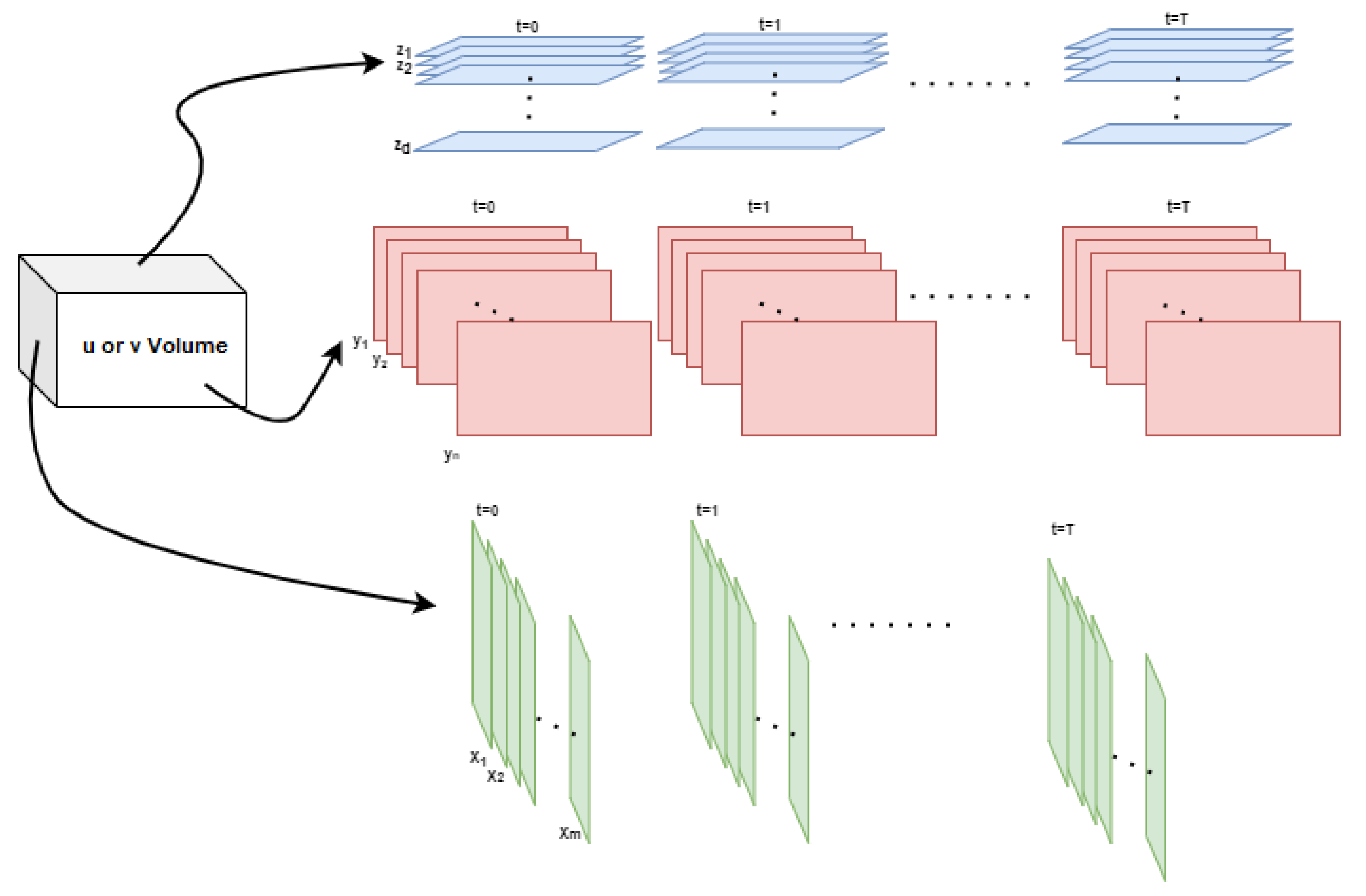
2.2. 4-Dimensional Tensor Slicing

The time series of the 3-dimensional gridded velocity forms a tensor whose dimensions must be reduced to one so it can be processed by the DL model. At each time step, a gridded velocity cube can be sliced in layers perpendicular to the three Cartesian coordinate axes (Figure 2). Thus, in the vertical direction (z-axis), the volume is split in horizontal layers corresponding to each depth level of the velocity data. Each layer becomes its own time series and can be reduced to a single dimension by EOF decomposition, as was carried out for the SSH field in [17]. For each resulting layer and velocity component, a DL model, trained on its own layer, is used to predict the evolution of that particular layer only. A similar approach can be used for layers perpendicular to the x and y axes and located at each grid point of the respective axis, as shown in Figure 2. As errors are specific to each layer and because the tensor evolves differently in each of the directions, it is expected that the models’ skill will vary with the direction of prediction, as explained in the following section.

Figure 2. Velocity plane field extractions perpendicular to each of the three Cartesian coordinate directions at each depth (z) in the vertical direction and at each grid point of the x (zonal direction) and y-axis (meridional direction), respectively.

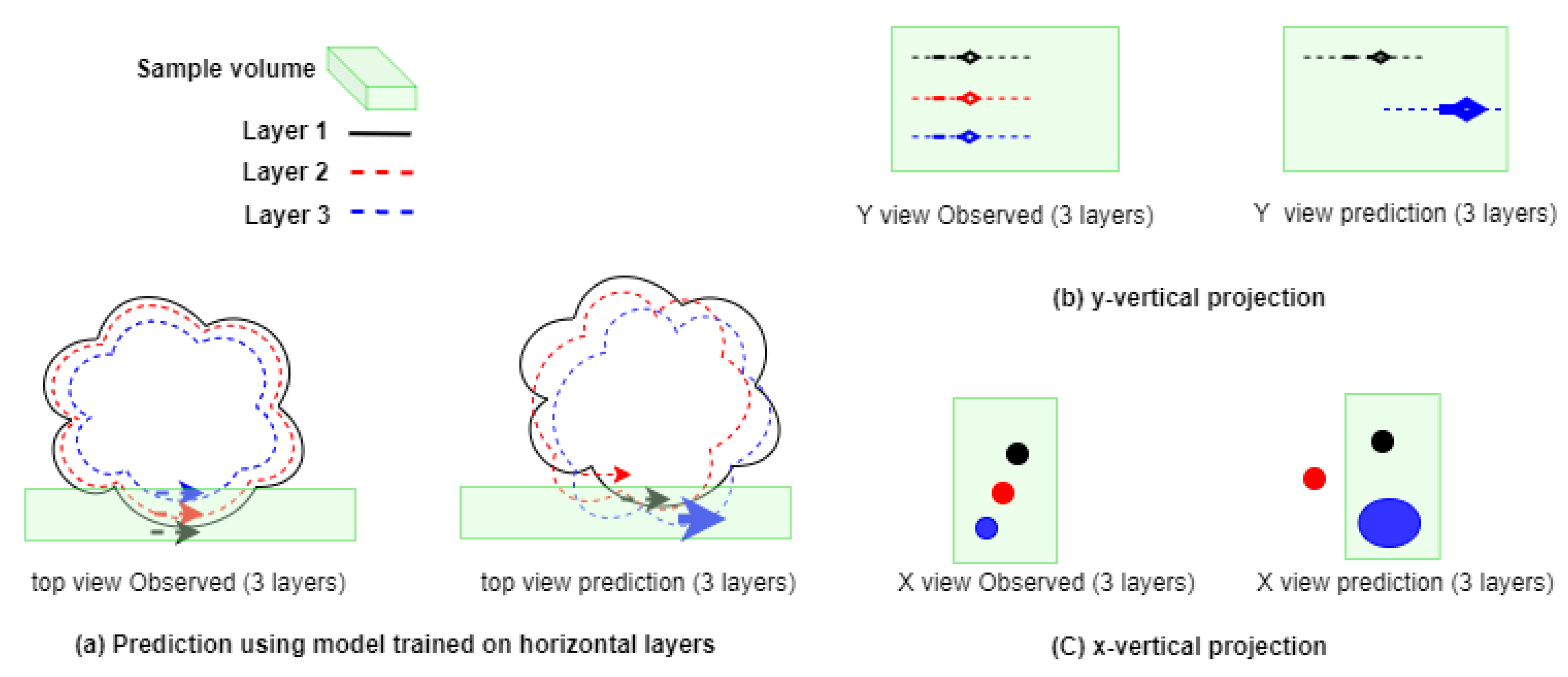
2.3. Volume Slicing Induced Errors

Most numerical model solutions are obtained from discretized partial differential equations solved on one or more embedded volumetric grid, such as the Arakawa C grid [34]. To solve these equations, boundary conditions are provided at the grid boundaries, where virtual grid points are added for computational purposes. Specific boundary conditions allow the radiation of features from within the grid to outside of it without losing the integrity of the signal inside the grid during the outing process. This process can be tracked in all three directions. In the case of a deep learning model, only features contained within the grid are available to the model. There is no influence from the boundaries, which serve to constrain the solution within the model and limit the model solution’s drift in numerical models. Therefore, DL model forecast errors in individual layers may grow significantly over time and ultimately change the integrity of the signal, as shown in Figure 3. This is particularly relevant in the case of perturbation simulations, where the phase of the signal in different layers could be changed by the errors in the individual layered predictions. Figure 3 provides an example of what it would look like in each of the planes normal to each direction. Starting with the z-planes (top view), a slight phase shift in the vertical direction will lead to the removal of the red signal in the x-plane in the region outlined by the green shaded area and also in the y-plane the furthest on the outside. As each forecast is sequentially reused for the next, the errors become part of the learning base. Additionally, because horizontal motions are much larger than vertical motions in the ocean, the DL model prediction skills will differ according to the direction of layers used for prediction.

Figure 3. Layered prediction-induced errors. (a) Top view, normal to the z-axis. (b) Lateral view normal to the y-axis. (c) Lateral view normal to the x-axis. The green shaded area highlights the focus area where errors are displayed. In each subplot, the left (right) image shows the observed (predicted) field. Each color corresponds to a different vertical layer as indicated, layer 1(3) being at the top (bottom).

To evaluate the layered prediction errors, the metrics set by GODAE OceanPredict [4] were applied. They identify two types of errors, namely the single point error and the structural error. These errors are quantified by the calculation of the Peak Signal to Noise Ratio (PSNR) including RMSE and correlation coefficient (CC) (see [17] for definitions), and Structural Similarity (SSIM), respectively. The PSNR is based on the mean square error (MSE) [35]. Given an observed plane field $Ob$ of size $m,n$ and its prediction $Pr$, MSE is defined as:

$$\mathrm{MSE}=\frac{1}{mn}\sum _{i=0}^{m-1}\sum _{j=0}^{n-1}{[Ob(i,j)-Pr(i,j)]}^2$$

(1)

The PSNR (in dB) is defined as:

$$\mathrm{PSNR}=10·{log}_{10}(\frac{{Peak}^2}{\mathrm{MSE}})$$

(2)

where $Peak$ is the maximum value of all data points in both $Ob$ and $Pr$. In image processing, PSNR is primarily used to assess the quality of an image reconstruction. The PSNR between two images is calculated in decibels. To compare image reconstruction quality, both the mean square error (MSE) and peak signal-to-noise ratio (PSNR) are often utilized.

The SSIM index can be calculated in sub-regions of each layer. It is a measure of similarity between two patterns [35].

$${\displaystyle \mathrm{SSIM}(Ob,Pr)=\frac{(2{\mu }_{Ob}{\mu }_{Pr}+c_1)(2{\sigma }_{ObPr}+c_2)}{({\mu }_{Ob}^2+{\mu }_{Pr}^2+c_1)({\sigma }_{Ob}^2+{\sigma }_{Pr}^2+c_2)}}$$

(3)

where:

• ${\mu }_{Ob}$ and ${\sigma }_{Ob}^2$ are the mean and variance of $Ob$, respectively.
• ${\mu }_{Pr}$ and ${\sigma }_{Pr}^2$ are the mean and the variance of $Pr$, respectively.
• ${\sigma }_{ObPr}$ is the covariance of $Ob$ and $Pr$.
• $c_1={\left(k_{1}L\right)}^2,c_2={\left(k_{2}L\right)}^2$ are used to stabilize the ratio with a weak denominator.
• $L=2^{\#bitspergridcell}-1$ is the dynamic range of the gridded velocity values.
• $k_1=0.01$ and $k_2=0.03$ are the default values of the two scale factors.

3. Deep Learning Prediction Model

Unlike conventional numerical models which use a set of a dynamical equations to describe a physical system, data-driven deep learning methods rely on neural networks to model physical systems. To achieve this, we first reduced the temporal matrix of each layer to one dimension by applying EOFs and then implemented an LSTM network to model the velocity field in each layer, as shown in Figure 4.

Figure 4. Single layer forecasting model flow chart.

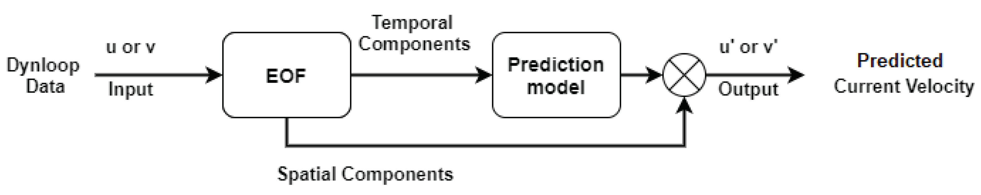
3.1. Empirical Orthogonal Functions

EOF is a major analysis tool in oceanographic, geophysical and meteorological applications [36,37,38]. EOFs are used to reduce data dimensions by separating spatial components from temporal components. The principle of this decomposition is to extract the most dominant information with fewer dimensions [39]. It provides a dense description of spatial data and temporal variability in terms of an orthogonal basis (eigenvectors). Each associated eigenvalue provides a measure of the fraction of the total variance under the EOF mode. This decomposition provides a statistical description of any dynamical processes by projecting them onto empirical normal modes, rather than the physical or natural modes of the system, which are process specific and therefore unable to encompass all the processes involved in the dynamics of the system being predicted in this study. The projection of the data onto EOF modes is called principal component (PC), which indicates the temporal variations of the variance of it associated spatial pattern [37]. EOF decomposition is carried out by Singular Value Decomposition (SVD), which is written as follows:

$$Q=UD{W}^T$$

(4)

where Q is an $n\times p$ matrix and D is an $n\times p$ rectangular diagonal matrix of non-negative numbers (the singular values of Q). U is an $n\times n$ matrix, the columns of which are orthogonal unit vectors of length n, called the left singular vectors of Q, and W is a $p\times p$ matrix whose columns are orthogonal unit vectors of length p and called the right singular vectors of Q. In addition, $UD$ is the time-dependent principal components ($PC$s), and $W^T$ is the spatial pattern matrix whose columns are so-called EOF modes.

3.2. Deep Learning Model: Long Short-Term Memory Network

The deep learning model selected for the prediction model is a type of Recurrent Neural Network (RNN). RNNs are well suited for time sequence prediction, and work by feeding the output of each neuron, along with a new input, back into itself, forming loops within its architecture [40]. In an RNN network, a simple RNN neuron or hidden unit’s output behavior can be modeled by Equation (5), where $x_n$ and $s_n$ are the input and state at time n, respectively. Furthermore, $W_{g_i}$ and $W_{g_s}$ represent the input and state (recurrence) weights and f an activation function. Note that the output can be obtained from the state whenever it is needed.

$$s_n=f\left(W_{g_i}{x}_{n-1}+W_{g_s}{s}_{n-1}\right)$$

(5)

However, the caveat of the RNN given in Equation (5) is its gradient vanishing problem or memory loss. This occurs because RNNs are typically trained with a stochastic gradient descent algorithm, and gradients may vanish for a multi-layer RNN due to the chain rule in differentiation. LSTM neural networks were designed to solve this problem [41], in which a memory unit $m_n$ was added to avoid the disappearance of gradients. Let $\alpha$ and $\beta$ be constants and ⊕ denote an element-wise multiplication; then, the memory unit is updated by the following rule:

$$m_n=\alpha \oplus m_{n-1}+\beta \oplus f\left(W_{g_i}{x}_{n-1}+W_{g_s}{s}_{n-1}\right)$$

(6)

The state is then related to the memory unit with an activation function. In this way, derivatives will not vanish due to the additive relationship described in Equation (6).

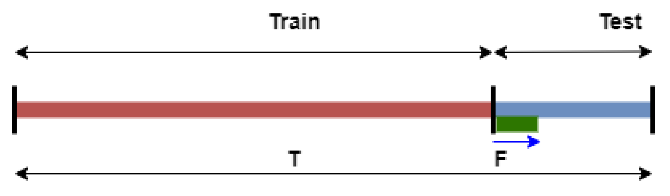
3.3. Prediction Procedure

The LSTM network used in this study was previously adopted for the prediction of SSH time series in [17,42]. In this study, two identical networks were designed to model and predict the velocity components, u and v, respectively. After the EOF decomposition of each velocity component, the PCs were used to train the LSTM model, which in turn was used to predict future PCs. At the beginning of the process, the system was initialized using random weights and then run through all the training data in chronological order, each time adjusting the weights through the gradient descent of the loss function. Each run through the entire training dataset is called an epoch and this step allows the model to optimize its weights (Equation (6)), at which point the model can predict any state learned from the data without the data at any point in time in hindcast mode.

The MATLAB Neural Network Toolbox was used to implement the LSTM network. The Adaptive Moment estimation [43] (Adam) optimization rather than the Stochastic Gradient Descent with Momentum [44] (SGDM) algorithm was used to update network weights iteratively during the training phase due to the improved performance with the former. The hyperparameters of the prediction model were manually tuned to optimize the performance of the prediction model. The resulting hyperparameters were as follows: mini-batch size = 128, initial learning rate = 0.03, number of hidden nodes = 100, and maximum number of Epochs = 500. Only one LSTM layer was used because the overall performance of the model, including the training and prediction processing time, as well as prediction skills, degraded when more layers were added. Training and prediction were carried out on a single NVIDIA GPU, TITAN X (Pascal compatibility) with CUDA toolkit Version 11 with a memory of 12GB. The training times for a single layer and for all layers for each direction are provided in Table 1. Once trained, at each prediction time step, the LSTM updates its state in accordance to its own prediction. This allows the LSTM to continue predicting based on both the training data and future predictions.

Table 1. Training time in seconds for a single and all layers in each directional model.

Training Direction	Single Layer	All Layers
Z direction	25.22 s	649.43 s
Y direction	26.32 s	722.8 s
X direction	25.16 s	652.15 s

The prediction procedure can be summarized as follows: (1) The current velocity components’ time series from time $t_1$ to $t_n$ are reduced to their respective PCs by EOF decomposition. (2) The PCs are used to train the LSTM model sequentially. (3) All the PCs up to time $t_n$ are then used to predict the PCs of the velocity field at time $t_n+1$. For the next prediction at time $t_n+2$, the predicted PCs at $t_n+1$ are used to retrain the LSTM model together with the PCs corresponding to time $t_1$ to $t_n$, and this is repeated for all subsequent forecasts. In addition, new data can be added at any time to the training dataset, which will then be used to retrain the LSTM model.

3.4. Layered Prediction Model Approach

As previously described, the water velocity dataset is a time series consisting of two orthogonal components u and v, each of which known as a four-dimensional tensor. To reduce the computational complexity, at each instant, the corresponding velocity cube (u or v) is partitioned into a number of layers (or planes). For each layer, a prediction module consisting of EOF and LSTM is trained and then used to predict the velocity field of that particular layer. Collectively, these prediction modules form a layered prediction model. Layered models are implemented for each spatial direction. As a consequence, they are referred to as prediction models X (29 layers), Y (36 layers), and Z (26 layers), respectively.

4. Layered Prediction Experiments

In all three directions, each layered model was trained using $90\%$ of the available time series and preserving the remaining for prediction validation. Thus, the training used 1629 samples (814.5 days) from 2 March 2009 to 25 May 2011, while the testing period started from 26 May 2011 to 23 August 2011 (90.5 days). The training and testing periods are illustrated in Figure 5. The model prediction period was set to 7 days, which was also the length of the sliding prediction window. This prediction period was chosen in response to the predictive skill goal set for the LC current speed by the United States’ National Academies of Sciences, Engineering, and Medicine (NASEM) [45].

Figure 5. Data partitioning for training and prediction experiments. T is the duration of the dataset (1810 time samples = 905 days), F the length of the prediction window (14 samples = 7 days), and the blue line is the testing period which includes 20 forecast sliding windows, each separated by a 12 h period.

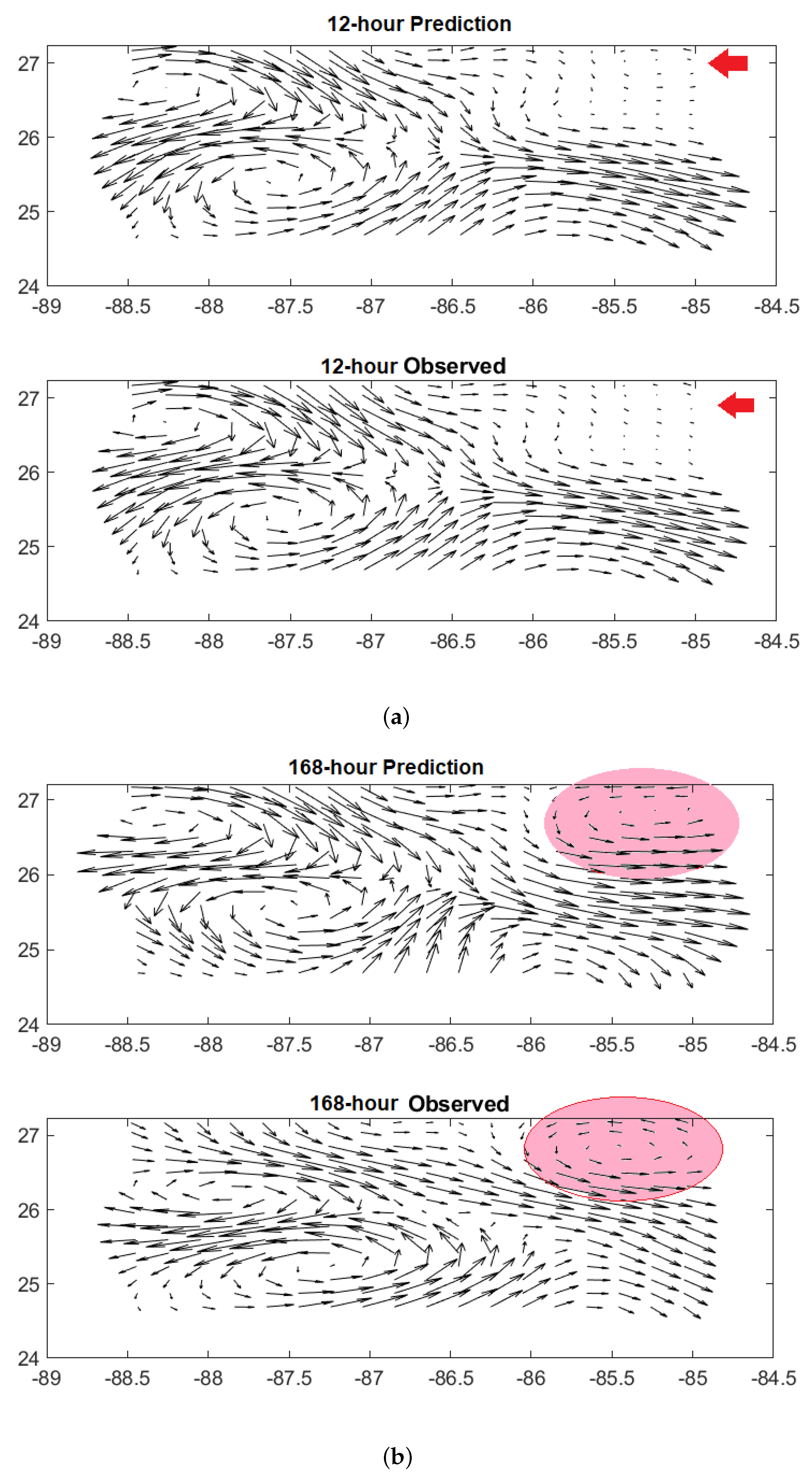
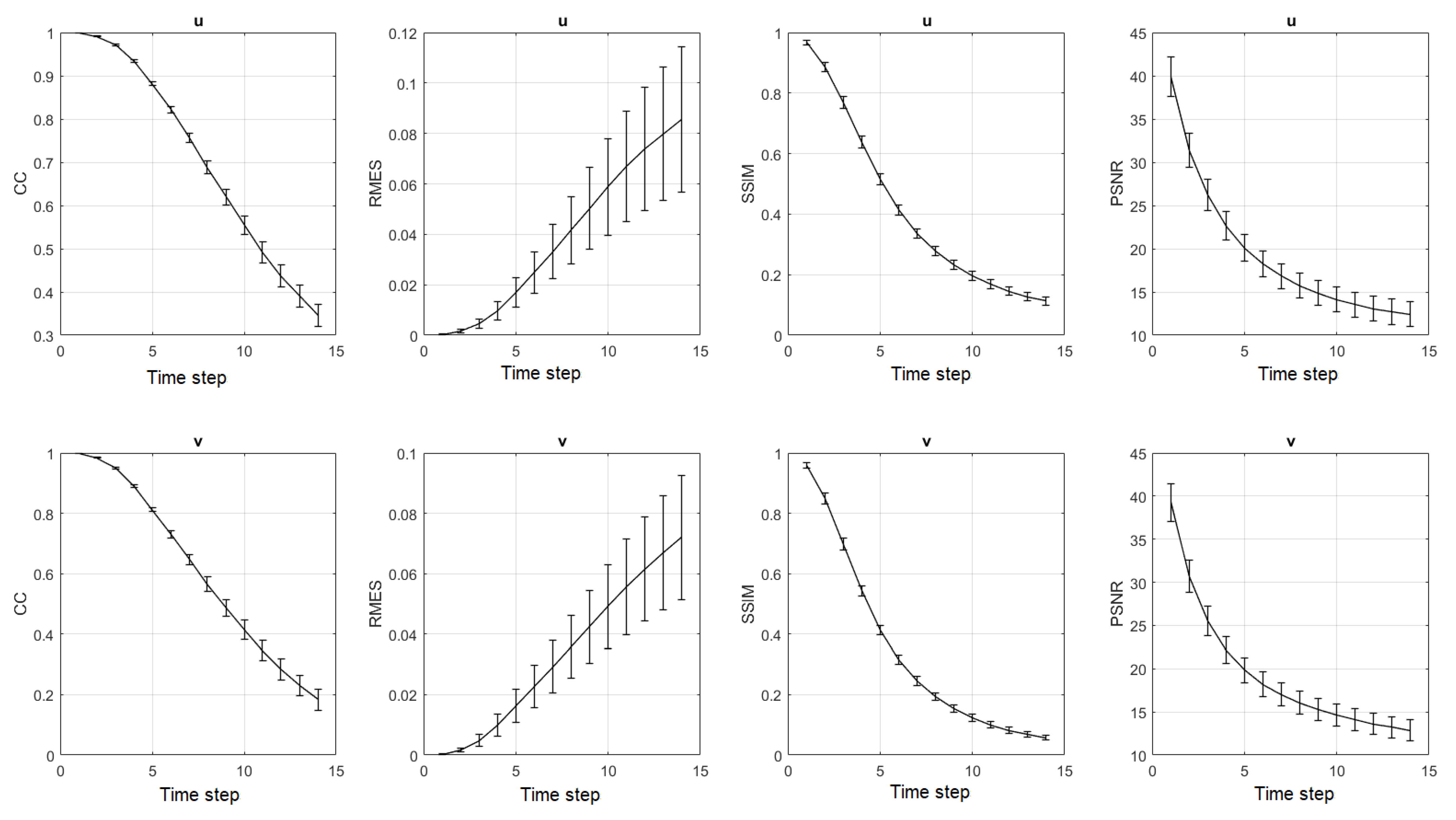
4.1. Model Z Velocity Predictions

Model Z, or the Z directional model, consisted of 26 horizontal layers distributed from the sea surface down to 500 m. The 7-day prediction of the model for the surface layer velocity (layer 1 in the z-direction) is shown in Figure 6. It illustrates that the proposed model was able to predict seven days in advance the formation of a cyclonic eddy in the region highlighted in Figure 6. The model accurately predicted the center of rotation, direction and strength of the velocity vectors at the surface. However, elsewhere, the model prediction differed more significantly from the observations. To assess the overall performance of the model, we computed the average CC, RMSE, SSIM and PSNR, along with their standard deviations, for both $u,v$ on each plane of each tensor and over the twenty sliding windows (Figure 7). These quantities quickly deteriorated over 14 time steps (7 days), which indicates the challenge of predicting LC velocity tensors compared to SSH prediction performed using a similar LSTM structure in [17,42,46], despite the fact that the cyclonic eddy was correctly predicted. Indeed, after 7 days, the anticyclone southwest of the predicted cyclone exhibited a weaker circulation than the observed one, and its northern counterpart was sustained for longer than the observed one.

Figure 6. Predicted (top) and corresponding observed (bottom) surface velocity. (a) Twelve-hour prediction. (b) One hundred sixty-eight-hour (7-day) prediction. The red arrows in (a) show the region of formation of the cyclonic eddy predicted in the red highlighted areas in (b).

Figure 7. Model Z fourteen time-step (7 days) 20-day sliding window average of CC, SSIM, PSNR, and RMSE of the velocity fields. The unit for the horizontal axis is prediction time steps (one time step is 12 h). The error bar denotes the standard deviation with a $95\%$ confidence interval.

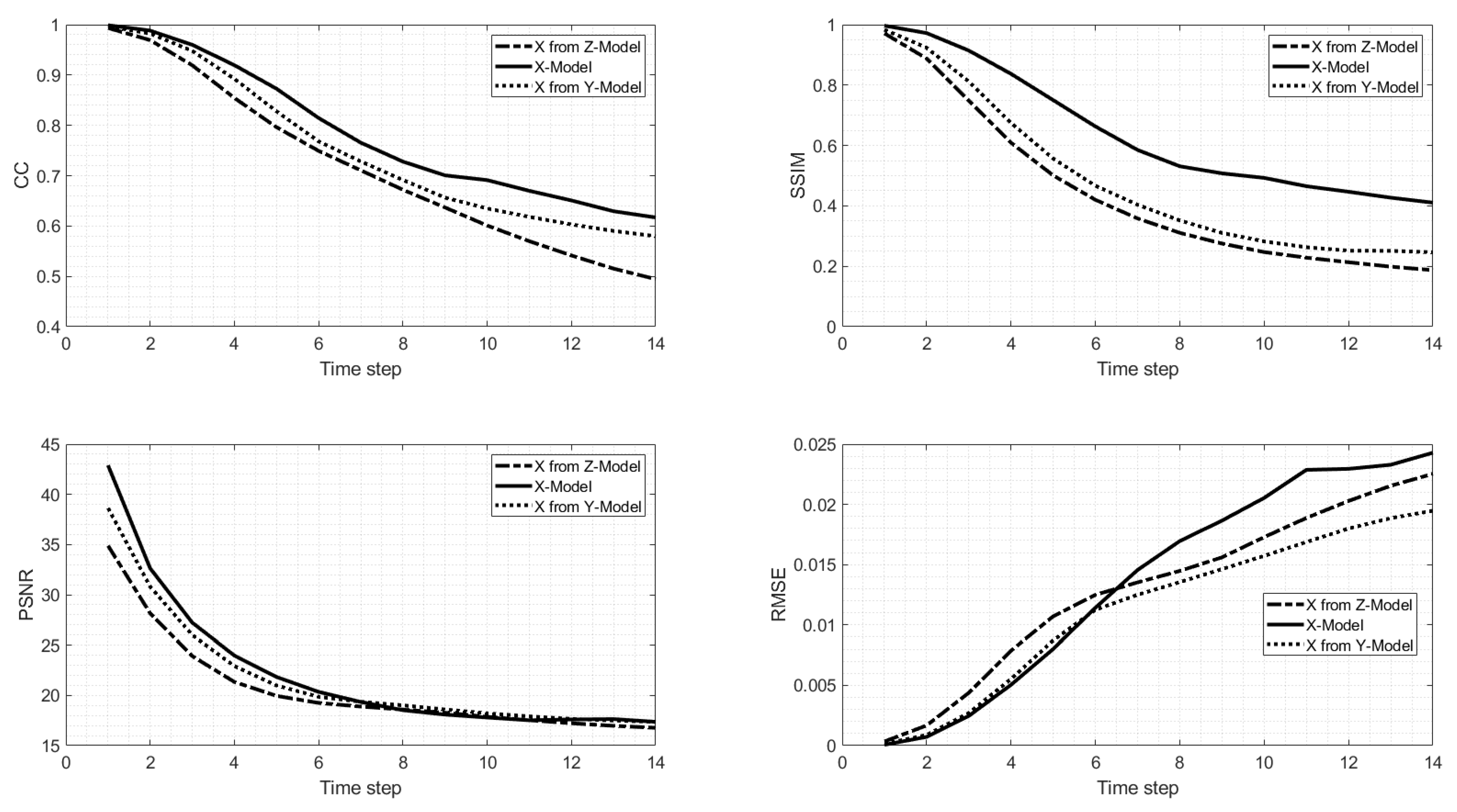
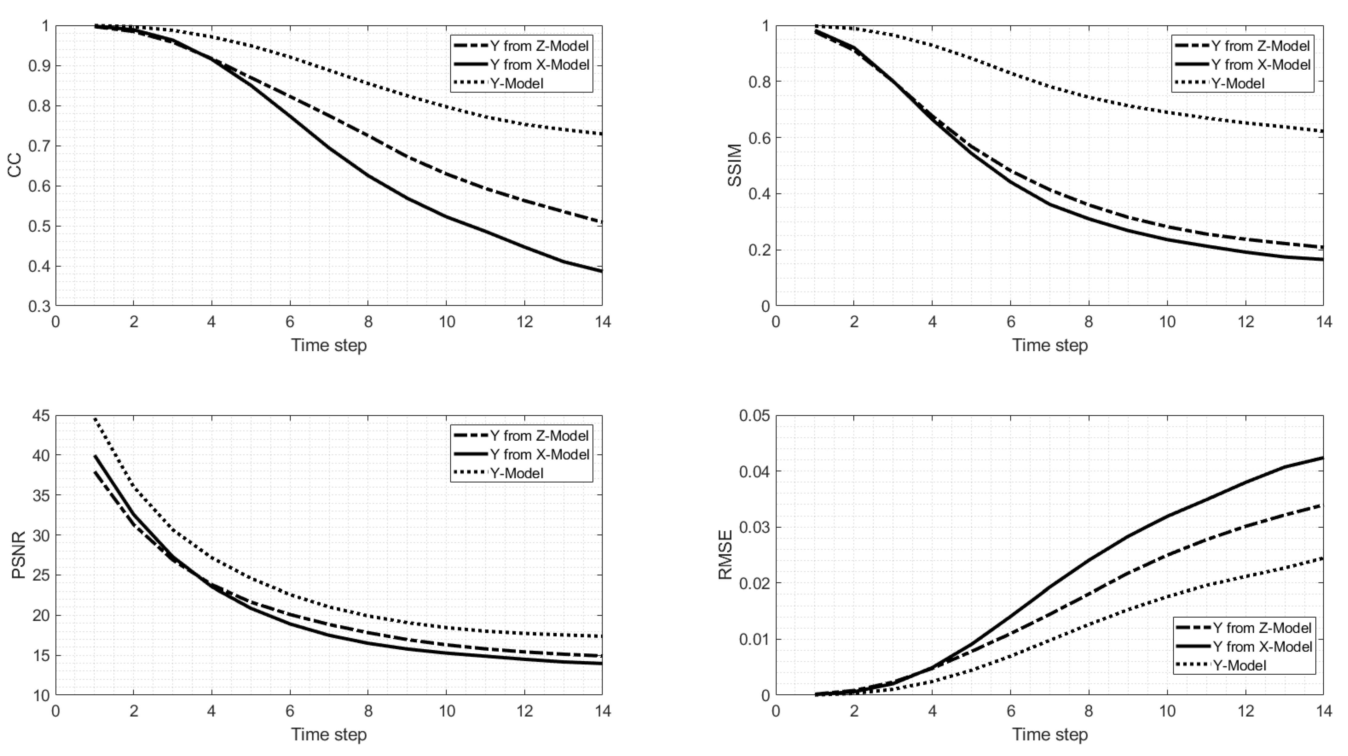
4.2. Directional Velocity Structure Prediction Dependency

We now compare the predictions of all models in each of the three Cartesian directions. In particular, for a given directional model prediction, we compared the other two model predictions along the same direction as the former. Figure 8 shows the comparison in terms of CC, RMSE, SSIM and PSNR for Model X prediction and the other two models (Models Y and Z) in the x-direction. All the metrics were calculated for fourteen time steps and averaged over 20-day sliding windows and over all the layers of the directional model. Model X prediction in the x-direction exhibited a higher CC and similarity index, although the PNSR is very similar between models, especially after the seventh time step. On the other hand, the RMSE is the highest for Model X after the sixth time step. Model Y prediction is also better than Model Z’s prediction in the x-direction.

Figure 8. Fourteen time-step (7 days) 20-day sliding window average of CC, SSIM, PSNR, and RMSE of the velocity fields in the x-direction, predicted by Model X (solid line), Model Y (dotted line), and Model Z (dashed line).

A similar comparison is shown for Model Y in Figure 9. The CC and the similarity index are strikingly much higher for Model Y and than for the other two models. The PSNR is also significantly higher and the RMSE much lower than for the other two models. The prediction of Model Z in the y-direction was also better than the one of Model X. In the x-directions, fewer differences were found between all three models predictions than in the y-direction.

Figure 9. Same as Figure 8 but for the velocity fields in the y-direction.

Figure 10 shows the comparison of the three models in the z-direction. As expected, Model Z is better at predicting in the z-direction; however it shows a better CC than for the other two models only after 7 days. The similarity index is much higher while the PSNR is similar to the ones of the other model, showing no significant improvement. The RMSE becomes lower than for the other two models after the seventh time step. Again, as for the x-direction prediction, the differences between the three models are not as different as they were in the y-direction. These results indicate that each model best prediction is associated with its direction of prediction. In addition, in terms of dynamical evolution, the most significant changes were in the y-direction (x-z planes) and better captured by the Model Y.

Figure 10. Same as Figure 8 but for the velocity fields in the z-direction.

4.3. Vertical Velocity Structure Prediction

Examples of the 7-day predicted flow field are shown in Figure 11, Figure 12 and Figure 13 for Models X, Y, and Z respectively. Figure 11 shows a vertical section of the velocity magnitude in the x-direction for all three models at 87${}^{\circ }$ W. It confirms the metrics results and shows the best agreement between the flow structure of Model X and the observations in the x-direction. Similarly, Figure 12 shows the vertical section of the velocity magnitude in the x-direction for all three models at 25${}^{\circ }$ N. It confirms the metrics results and shows the best agreement between the flow structure of Model Y and the observations in the y-direction. The same consistency between the prediction and observed flow structure is also confirmed for Model Z in the z-direction (Figure 13). As each prediction model performs best in its corresponding tensor orientation, we propose fusing the prediction of all three models into one tensor.

Figure 11. Vertical section of the velocity tensor in the x-direction at 87${}^{\circ }$ N on day 7 of the prediction. (a) Observations; (b) Model X prediction; (c) Model Y prediction; (d) Model Z prediction.

Figure 12. Vertical section of the velocity tensor in the y-direction at 25${}^{\circ }$ W.

Figure 13. Horizontal section of the velocity tensor at 100 m depth on day 7 of the prediction. (a) Observations; (b) Model X prediction; (c) Model Y prediction; (d) Model Z prediction.

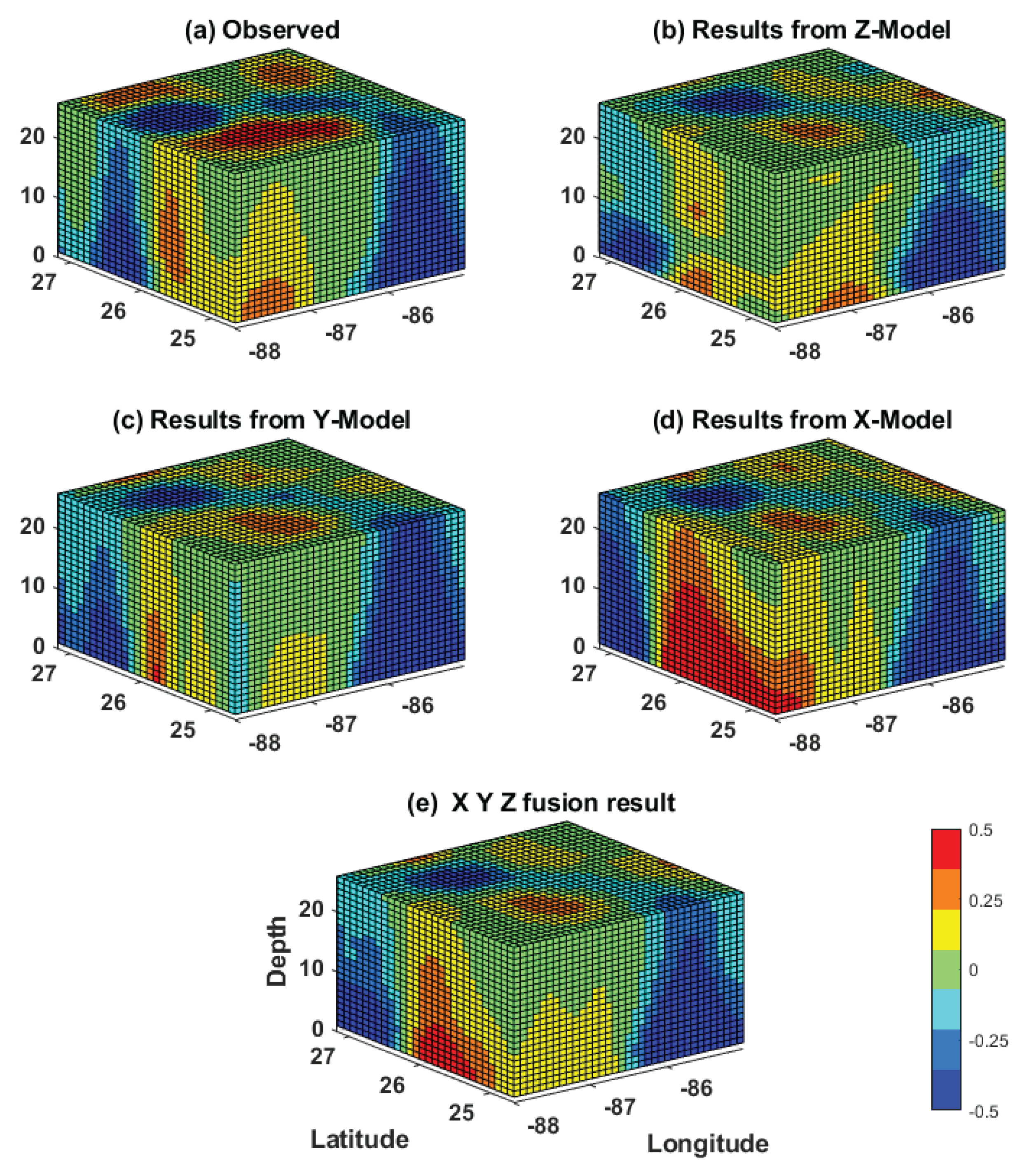
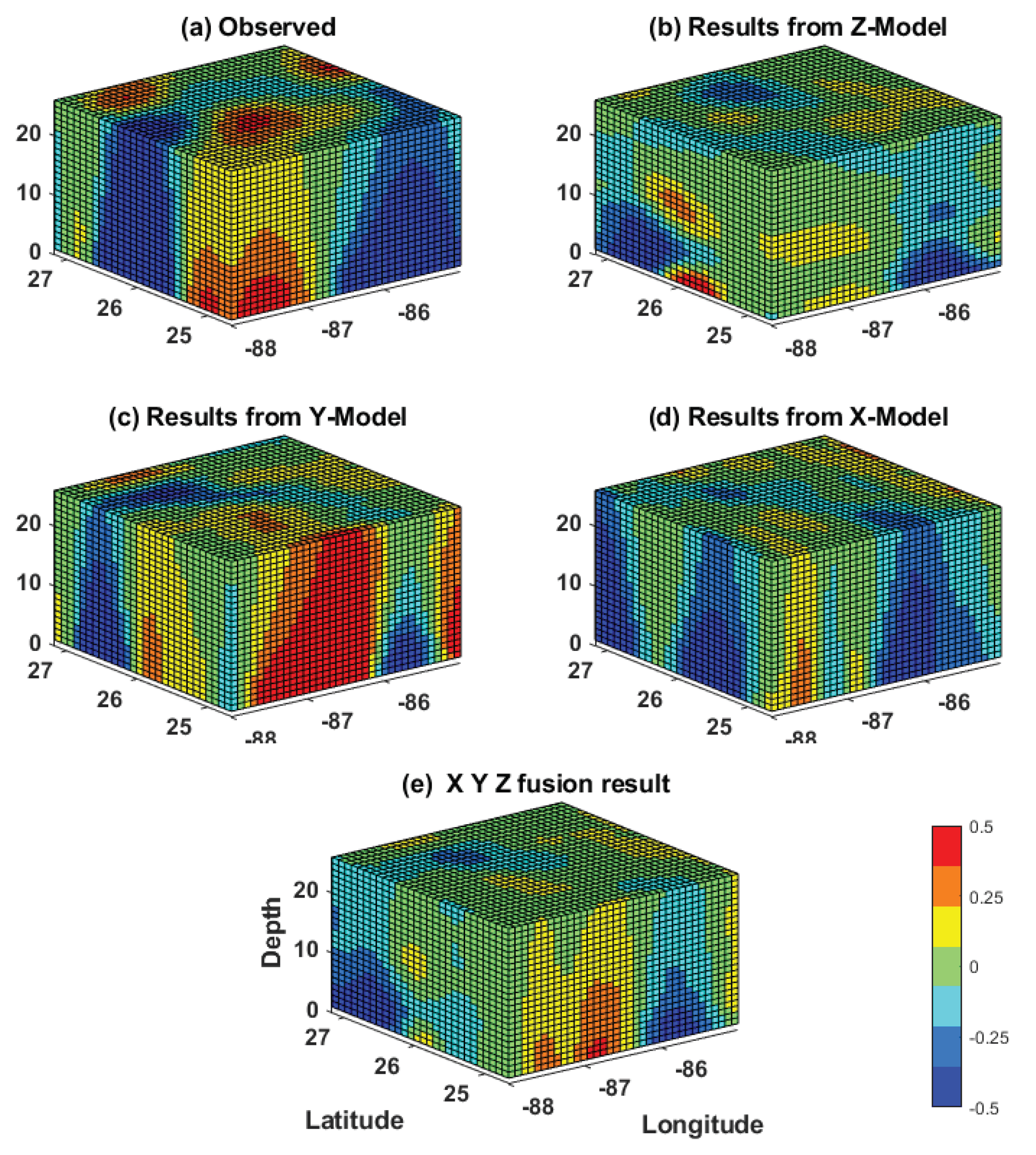
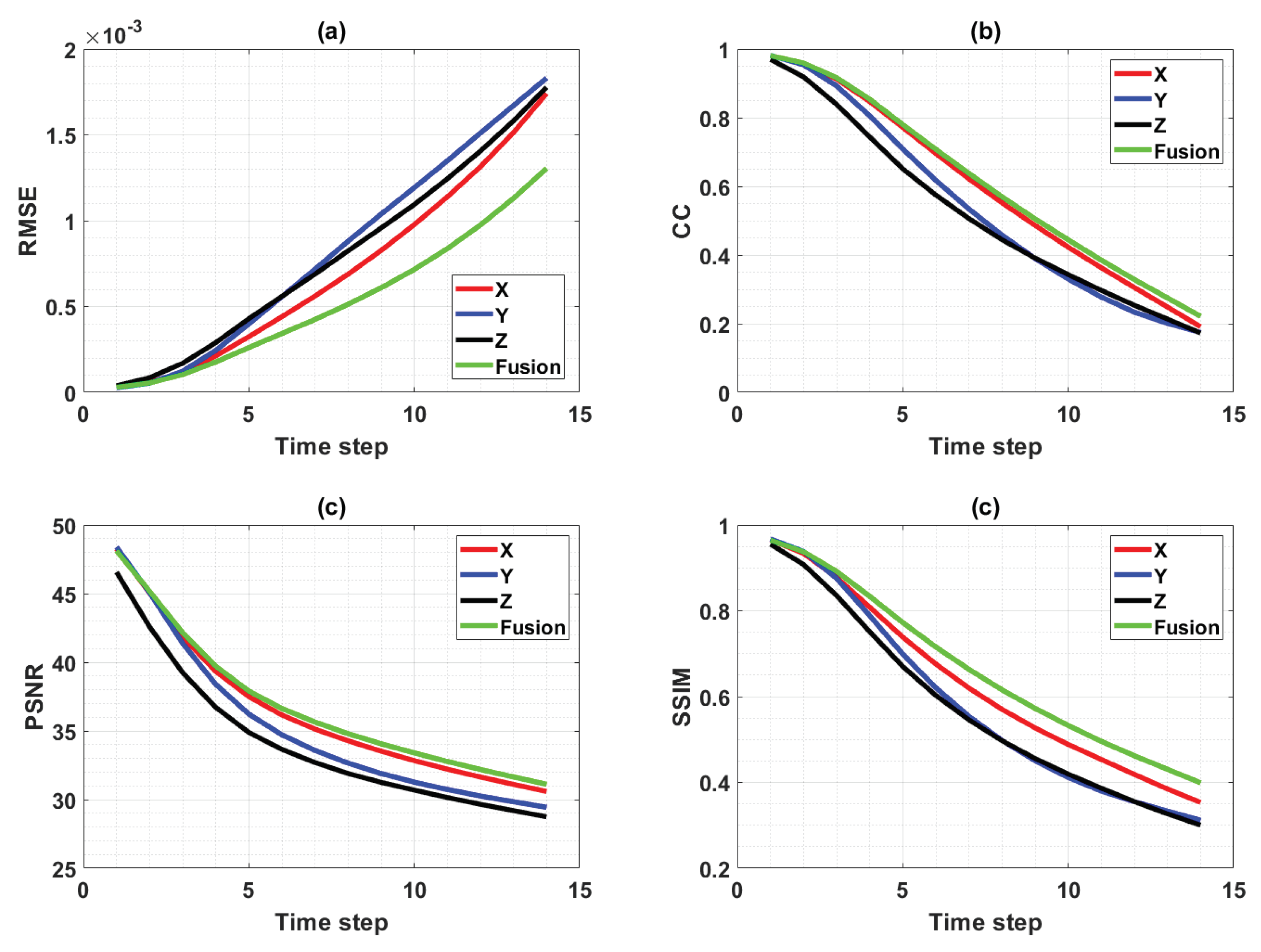
4.4. Fusion of the Models’ Predictions

As each model can best predict the evolution of the velocity field in its respective layers, we hypothesize that the fusion of the three model predictions would yield an improved prediction of the overall tensor over each individual one. For this purpose, a simple fusion block was added to the prediction system, as shown in Figure 14. Although various methods can be used to fuse all three tensors, such as unweighted or median selection-based average, we chose to apply a three-dimensional Gaussian smoothing procedure [47] as it provides better results than the other two. The results of the fusion process are shown for the 72 h (3-day) and 168 h (7-day) predictions in Figure 15 and Figure 16, respectively. These figures consist of a 3D representation of the normalized relative vorticity of the flow predicted by each of the three individual models and by the fusion method. Despite the noise associated with each model, the fusion approach is able to filter the noise out and deliver a tensor field that is very similar to the observations, even for a 168 h prediction. The significant improvement of the 3D tensor prediction by the fusion process over individual prediction models is further demonstrated by computing the metrics RMSE, PNSR, SSIM and CC of the various predictions (Figure 17). The fusion output showed an overall improvement over individual predictions for all metrics over the 7-day prediction window. In particular, the RMSE was reduced by more than 25% on day 7 of the prediction.

Figure 14. Block diagram of the fusion approach to produce a unified volumetric prediction.

Figure 15. Three-dimensional normalized relative vorticity field of the observed and 72 h predicted tensors. (a) Observed, (b) Model Z, (c) Model X, (d) Model Y, (e) and fusion result.

Figure 16. The conditions are same as Figure 15 for the 168 h prediction.

Figure 17. Fusion results. (a) Mean Squared Error (MSE), (b) Correlation Coefficient (CC), (c) Peak Signal-to-Noise Ratio (PNSR) and (d) Structural Similarity index (SSIM) between the observed 3-dimensional fields and the predictions from Models Z, X, and Y.

5. Conclusions

Modeling and predicting the LCS subsurface vertical structure in the GoM region is essential to all aspects of life in the region. However, useful forecasts of the flow field by current modeling methods do not exceed two days [5,6,7]. In this study, we developed a deep learning-based prediction model that was capable of predicting some important features of the 3D velocity fields of the LCS up to seven days in advance in a rectangular region where the LC is most active and commonly sheds eddies (Figure 6). Overall, the fusion model exhibited a CC > 0.5 up to 4.5 days (Figure 17). Subsurface velocity data measured by in-situ sensors for an approximately three-year period [29] were used to train and test a deep learning prediction method. To implement the deep learning model, we reduced the dimensionality of the tensors of each component of the velocity field to one dimension by applying EOF. The obtained PC vectors were used as an input variable to the LSTM model. The prediction model was applied separately to each layer of the tensor. We defined one tensor for each direction of the Cartesian coordinate system, which led to three prediction models associated with each direction, respectively. Each model was composed of one individual LSTM model per layer in each tensor and the final prediction consisted of the final tensor made of all the layered predictions for each velocity component. The results of this approach revealed that the prediction models associated with each of the three directions were the best at predicting the flow field in their respective directions. The errors across layers significantly altered the cross-layer structure of the flow. However, the fusion of all three models’ solution with a Gaussian filter delivered an improved prediction field over each individual predictions.

Because the number of layer models necessary to conduct the full three-dimensional prediction is equal to the total number of grid points of the field to be predicted, the implementation of such model for real-time forecast seems unrealistic. However, multithread and parallel computing allows for the simultaneous computation of the predictions in all the layers in an efficient and timely manner. In addition, such dense observation arrays are rare and spatially and temporally limited, which limits the size and number of the layers to be predicted as well. In any case, when compared to ocean numerical model operations, even though numerical models are much cheaper to operate, they are unable to reliably predict the evolution of the ocean state without being constrained by ocean observations. It is true that observing arrays are ephemeral, but when they do exist they can be used to make forecasts that do not require numerical models, which simplifies the data processing and streamlines the forecasting process since only one variable is used versus the multitude of state and atmospheric variables required by ocean numerical models. Table 1 shows that the computational time for training is less than 800 s for all layers in a given direction. Assuming that each direction can be computed by one thread, then the overall prediction time would be less than 800 s, which makes this approach adequate for real-time forecasting, even at a hourly rate. HF radar ocean surface current measurements provide a good test-bed for the application of our method, where in this case, only one layer is predicted. The latter are now increasingly used for monitoring coastal circulation in many areas of the coast around the world [48]. The other limitation of the deep learning method is the duration of the measurements. Such methods’ accuracy strongly depends on the diversity of events captured by the measurements and therefore their prediction skills can be limited by the duration of the measurements used to create the deep learning models. Ideally, a times series that captures the full extent of the variability in the natural system would yield the best forecast by such methods. However, it is not explicitly clear how prediction improvement is correlated to the duration of the measurements in this tensor prediction method. In a point-wise prediction exercise of ocean current velocity for unmanned underwater vehicle navigation, Immas et al. [12] showed that they could predict with an LSTM model one month of current with one month of training data.

The layered prediction method applied in this study was originally developed by Wang et al. [17] to predict the evolution of the SSH, a two-dimensional field. Predicting the three-dimensional velocity fields with this two-dimensional method has revealed the importance of the relative changes between layers in the accuracy of the predicted tensor. Future work will be focused on the inclusion of the relationship between individual nodes and their surrounding nodes in the domain, in order to account for the relative evolution between nodes. This node’s spatio-temporal connectivity could be learned through another DL model ultimately coupled with the prediction model. We anticipate that such multi-model approach could provide longer reliable three-dimensional forecasts than the approach herein.

References

- Smith, N. The global ocean data assimilation experiment (GODAE). In Proceedings of the Monitoring the Oceans in the 2000s: An Integrated Approach, Biarritz, France, 15–17 October 1997. [Google Scholar]
- Schiller, A.; Davidson, F.; DiGiacomo, P.M.; Wilmer-Becker, K. Better Informed Marine Operations and Management: Multidisciplinary Efforts in Ocean Forecasting Research for Socioeconomic Benefit. Bull. Am. Meteorol. Soc. 2016, 97, 1553–1559. [Google Scholar] [CrossRef] [Green Version]
- Vinayachandran, P.N.; Davidson, F.; Chassignet, E.P. Toward Joint Assessments, Modern Capabilities, and New Links for Ocean Prediction Systems. Bull. Am. Meteorol. Soc. 2020, 101, E485–E487. [Google Scholar] [CrossRef] [Green Version]
- MERSEA IP. List of Internal Metrics for the MERSEA-GODAE Global Ocean: Specification for Implementation; Mercator Ocean: Ramonville Saint-Agne, France, 14 March 2006; Available online: https://www.clivar.org/sites/default/files/documents/wgomd/GODAE_MERSEA-report.pdf (accessed on 12 September 2021).
- Chao, Y.; Li, Z.; Farrara, J.; McWilliams, J.C.; Bellingham, J.; Capet, X.; Chavez, F.; Choi, J.K.; Davis, R.; Doyle, J.; et al. Development, implementation and evaluation of a data-assimilative ocean forecasting system off the central California coast. Deep Sea Res. Part II Top. Stud. Oceanogr. 2009, 56, 100–126. [Google Scholar] [CrossRef]
- Shulman, I.; Paduan, J.D. Assimilation of HF radar-derived radials and total currents in the Monterey Bay area. Deep Sea Res. Part II Top. Stud. Oceanogr. 2009, 56, 149–160. [Google Scholar] [CrossRef] [Green Version]
- Cooper, C.; Danmeier, D.; Frolov, S.; Stuart, G.; Zuckerman, S.; Anderson, S.; Sharma, N. Real Time Observing and Forecasting of Loop Currents in 2015. In Proceedings of the Offshore Technology Conference, Houston, TX, USA, 2–5 May 2016. [Google Scholar] [CrossRef]
- LeCun, Y.; Bengio, Y.; Hinton, G. Deep learning. Nature 2015, 521, 436–444. [Google Scholar] [CrossRef]
- Hochreiter, S.; Schmidhuber, J. Long short-term memory. Neural Comput. 1997, 9, 1735–1780. [Google Scholar] [CrossRef]
- Salehinejad, H.; Sankar, S.; Barfett, J.; Colak, E.; Valaee, S. Recent advances in recurrent neural networks. arXiv 2017, arXiv:1801.01078. [Google Scholar]
- Al-Rfou, R.; Choe, D.; Constant, N.; Guo, M.; Jones, L. Character-Level Language Modeling with Deeper Self-Attention. Proc. AAAI Conf. Artif. Intell. 2019, 33, 3159–3166. [Google Scholar] [CrossRef] [Green Version]
- Immas, A.; Do, N.; Alam, M.R. Real-time in situ prediction of ocean currents. Ocean Eng. 2021, 228, 108922. [Google Scholar] [CrossRef]
- Banan, A.; Nasiri, A.; Taheri-Garavand, A. Deep learning-based appearance features extraction for automated carp species identification. Aquac. Eng. 2020, 89, 102053. [Google Scholar] [CrossRef]
- Shamshirband, S.; Rabczuk, T.; Chau, K.W. A Survey of Deep Learning Techniques: Application in Wind and Solar Energy Resources. IEEE Access 2019, 7, 164650–164666. [Google Scholar] [CrossRef]
- Muhamed Ali, A.; Zhuang, H.; Ibrahim, A.; Oneeb, R.; Huang, M.; Wu, A. A machine learning approach for the classification of kidney cancer subtypes using mirna genome data. Appl. Sci. 2018, 8, 2422. [Google Scholar] [CrossRef] [Green Version]
- Fan, Y.; Xu, K.; Wu, H.; Zheng, Y.; Tao, B. Spatiotemporal modeling for nonlinear distributed thermal processes based on KL decomposition, MLP and LSTM network. IEEE Access 2020, 8, 25111–25121. [Google Scholar] [CrossRef]
- Wang, J.L.; Zhuang, H.; Chérubin, L.M.; Ibrahim, A.K.; Muhamed Ali, A. Medium-Term Forecasting of Loop Current eddy Cameron and eddy Darwin formation in the Gulf of Mexico with a Divide-and-Conquer Machine Learning Approach. J. Geophys. Res. Oceans 2019, 124, 5586–5606. [Google Scholar] [CrossRef]
- Dukhovskoy, D.; Leben, R.; Chassignet, E.; Hall, C.; Morey, S.; Nedbor-Gross, R. Characterization of the uncertainty of loop current metrics using a multidecadal numerical simulation and altimeter observations. Elsevier 2015, 100, 140–158. [Google Scholar] [CrossRef]
- Donohue, K.A.; Watts, D.; Hamilton, P.; Leben, R.; Kennelly, M. Loop Current Eddy formation and baroclinic instability. Dyn. Atmos. Ocean. 2016, 76, 195–216. [Google Scholar] [CrossRef] [Green Version]
- Vukovich, F.M.; Maul, G.A. Cyclonic eddies in the eastern Gulf of Mexico. J. Phys. Oceanogr. 1985, 15, 105–117. [Google Scholar] [CrossRef]
- Sturges, W.; Leben, R. Frequency of Ring Separations from the Loop Current in the Gulf of Mexico: A Revised Estimate. J. Phys. Oceanogr. 2000, 30, 1814–1819. [Google Scholar] [CrossRef]
- Leben, R.R. Altimeter-derived loop current metrics. Geophys. Monogr. Am. Geophys. Union 2005, 161, 181. [Google Scholar]
- Chérubin, L.M.; Sturges, W.; Chassignet, E.P. Deep flow variability in the vicinity of the Yucatan Straits from a high-resolution numerical simulation. J. Geophys. Res. Ocean. 2005, 110. [Google Scholar] [CrossRef] [Green Version]
- Chérubin, L.M.; Morel, Y.; Chassignet, E.P. Loop Current Ring Shedding: The Formation of Cyclones and the Effect of Topography. J. Phys. Oceanogr. 2006, 36, 569–591. [Google Scholar] [CrossRef]
- Oey, L.; Ezer, T.; Lee, H. Loop Current, rings and related circulation in the Gulf of Mexico: A review of numerical models and future challenges. Geophys. Monogr. Am. Geophys. Union 2005, 161, 31. [Google Scholar]
- Chassignet, E.; Hurlburt, H.; Metzger, E.; Smedstad, O.; Cummings, A.; Halliwell, G.; Bleck, R.; Baraille, R.; Wallcraft, A.; Lozano, C.; et al. US GODAE: Global Ocean Prediction with the HYbrid Coordinate Ocean Model (HYCOM). Oceanography 2009, 22, 64–75. [Google Scholar] [CrossRef]
- Rowley, C.; Mask, A. Regional and coastal prediction with the Relocatable Ocean Nowcast/Forecast System. Oceanography 2014, 27, 44–55. [Google Scholar] [CrossRef] [Green Version]
- Gopalakrishnan, G.; Cornuelle, B.D.; Hoteit, I.; Rudnick, D.L.; Owens, W.B. State estimates and forecasts of the loop current in the Gulf of Mexico using the MITgcm and its adjoint. J. Geophys. Res. Ocean. 2013, 118, 3292–3314. [Google Scholar] [CrossRef] [Green Version]
- Hamilton, P.; Lugo-Fernández, A.; Sheinbaum, J. A Loop Current experiment: Field and remote measurements. Dyn. Atmos. Ocean. 2016, 76, 156–173. [Google Scholar] [CrossRef]
- Donohue, K.A.; Watts, D.R.; Tracey, K.L.; Greene, A.D.; Kennelly, M. Mapping circulation in the Kuroshio Extension with an array of current and pressure recording inverted echo sounders. J. Atmos. Ocean. Technol. 2010, 27, 507–527. [Google Scholar] [CrossRef] [Green Version]
- Daley, R. Atmospheric Data Analysis; Number 2; Cambridge University Press: Cambridge, UK, 1993. [Google Scholar]
- Watts, D.R.; Sun, C.; Rintoul, S. A two-dimensional gravest empirical mode determined from hydrographic observations in the Subantarctic Front. J. Phys. Oceanogr. 2001, 31, 2186–2209. [Google Scholar] [CrossRef]
- Suranjana, S.; Moorthi, S.; Pan, H.; Wu, X.; Wang, J.; Nadiga, S.; Tripp, P.; Kistler, R.; Woollen, J.; Behringer, D.; et al. The NCEP climate forecast system reanalysis. Bull. Am. Meteorol. Soc. 2010, 91, 1015–1057. [Google Scholar]
- Arakawa, A.; Lamb, V.R. Computational Design of the Basic Dynamical Processes of the UCLA General Circulation Model. Methods in Computational Physics. Adv. Res. Appl. 1977, 17, 173–265. [Google Scholar] [CrossRef]
- Wang, Z.; Bovik, A.C.; Sheikh, H.R.; Simoncelli, E.P. Image quality assessment: From error visibility to structural similarity. IEEE Trans. Image Process. 2004, 13, 600–612. [Google Scholar] [CrossRef] [Green Version]
- Zeng, X.; Li, Y.; He, R. Predictability of the loop current variation and eddy shedding process in the Gulf of Mexico using an artificial neural network approach. J. Atmos. Ocean. Technol. 2015, 32, 1098–1111. [Google Scholar] [CrossRef] [Green Version]
- Casagrande, G.; Stephan, Y.; Varnas, A.C.W.; Folegot, T. A novel empirical orthogonal function (EOF)-based methodology to study the internal wave effects on acoustic propagation. IEEE J. Ocean. Eng. 2011, 36, 745–759. [Google Scholar] [CrossRef]
- Beckers, J.M.; Rixen, M. EOF calculations and data filling from incomplete oceanographic datasets. J. Atmos. Ocean. Technol. 2003, 20, 1839–1856. [Google Scholar] [CrossRef]
- Thomson, R.E.; Emery, W.J. Data Analysis Methods in Physical Oceanography; Newnes: Amsterdam, The Netherlands, 2014. [Google Scholar]
- Yin, W.; Kann, K.; Yu, M.; Schütze, H. Comparative Study of CNN and RNN for Natural Language Processing. arXiv 2017, arXiv:1702.01923. [Google Scholar]
- Bengio, Y.; Simard, P.; Frasconi, P. Learning long-term dependencies with gradient descent is difficult. IEEE Trans. Neural Netw. 1994, 5, 157–166. [Google Scholar] [CrossRef] [PubMed]
- Ali, A.M.; Zhuang, H.; Ibrahim, A.K.; Wang, J.L. Preliminary results of forecasting of the loop current system in Gulf of Mexico using robust principal component analysis. In Proceedings of the 2018 IEEE International Symposium on Signal Processing and Information Technology (ISSPIT), Louisville, KY, USA, 6–8 December 2018; pp. 1–5. [Google Scholar] [CrossRef]
- Kingma, D.P.; Ba, J. Adam: A method for stochastic optimization. arXiv 2014, arXiv:1412.6980. [Google Scholar]
- Murphy, K.P. Machine Learning: A Probabilistic Perspective; MIT Press: Cambridge, MA, USA, 2012. [Google Scholar]
- National Academies of Sciences Engineering and Medicine. Understanding and Predicting the Gulf of Mexico Loop Current: Critical Gaps and Recommendations; National Academies Press: Washington, DC, USA, 2018. [Google Scholar]
- Wang, J.L.; Zhuang, H.; Chérubin, L.; Muhamed Ali, A.; Ibrahim, A. Loop Current SSH Forecasting: A New Domain Partitioning Approach for a Machine Learning Model. Forecasting 2021, 3, 570–579. [Google Scholar] [CrossRef]
- Haddad, R.A.; Akansu, A.N. A class of fast Gaussian binomial filters for speech and image processing. IEEE Trans. Signal Process. 1991, 39, 723–727. [Google Scholar] [CrossRef]
- Harlan, J.; Terrill, E.; Hazard, L.; Keen, C.; Barrick, D.; Whelan, C.; Howden, S.; Kohut, J. The Integrated Ocean Observing System high-frequency radar network: Status and local, regional, and national applications. Mar. Technol. Soc. J. 2010, 44, 122–132. [Google Scholar] [CrossRef] [Green Version]
Publisher’s Note: MDPI stays neutral with regard to jurisdictional claims in published maps and institutional affiliations. |
© 2021 by the authors. Licensee MDPI, Basel, Switzerland. This article is an open access article distributed under the terms and conditions of the Creative Commons Attribution (CC BY) license (https://creativecommons.org/licenses/by/4.0/).