Article

Landslide Forecast by Time Series Modeling and Analysis of High-Dimensional and Non-Stationary Ground Motion Data

School of Mathematics and Statistics, University of Melbourne, Parkville 3010, Australia
*
Author to whom correspondence should be addressed.
These authors contributed equally to this work.
Forecasting 2021, 3(4), 850-867; https://doi.org/10.3390/forecast3040051
Submission received: 7 September 2021 / Revised: 8 November 2021 / Accepted: 8 November 2021 / Published: 12 November 2021

Abstract

:
High-dimensional, non-stationary vector time-series data are often seen in ground motion monitoring of geo-hazard events, e.g., landslides. For timely and reliable forecasts from such data, we developed a new statistical approach based on two advanced econometric methods, i.e., error-correction cointegration (ECC) and vector autoregression (VAR), and a newly developed dimension reduction technique named empirical dynamic quantiles (EDQ). Our ECC–VAR–EDQ method was born by analyzing a big landslide dataset, comprising interferometric synthetic-aperture radar (InSAR) measurements of ground displacement that were observed at 5090 time states and 1803 locations on a slope. The aim was to develop an early warning system for reliably forecasting any impending slope failure whenever a precursory slope deformation is on the horizon. Specifically, we first reduced the spatial dimension of the observed landslide data by representing them as a small set of EDQ series with negligible loss of information. We then used the ECC–VAR model to optimally fit these EDQ series, from which forecasts of future ground motion can be efficiently computed. Moreover, our method is able to assess the future landslide risk by computing the relevant probability of ground motion to exceed a red-alert threshold level at each future time state and location. Applying the ECC–VAR–EDQ method to the motivating landslide data gives a prediction of the incoming slope failure more than 8 days in advance.

1. Introduction

Geo-hazard events, including earthquakes and landslides, can present significant damage to the environment and society; cf. [1,2]. Developing the capability to reliably predict the imminent occurrence of such a disaster is crucial for enhancing society’s preparedness and mitigating the disaster’s impact. However, behaviors of the geological processes underpinning such geo-hazard events are mostly complicated in both space and time, in that the multivariate time series data collected from monitoring these processes by modern techniques, such as interferometric synthetic-aperture radar (InSAR), are often high-dimensional and non-stationary. To date, there exist few statistical methods capable of analyzing high-dimensional non-stationary InSAR time series for timely and reliable forecasts of geo-hazard events [3]. It was therefore the goal of this research to develop an effective statistical method for modeling high-dimensional, non-stationary vector time series and accordingly for timely forecasting with precision. The capability of the method was tested on a real landslide dataset detailed in [4]. Briefly, the landslide dataset comprises 1803 time series of InSAR data on ground displacement, observed every 6 min for 5090 times and at 1803 locations.
Analyzing multivariate time series is often based on a vector auto-regression (VAR) model framework; see Chapter 2 in [5]. A prerequisite for the parameter estimation involved in the VAR-based analysis to be statistically consistent is that the underlying multivariate time series be stationary. This condition is, however, not satisfied for our landslide data which can be shown to be unit-root non-stationary with significant statistical evidence. Therefore, we cannot use the VAR model to consistently fit the landslide data and estimate the involved parameters directly. Instead, we resort to searching for certain linear transformation of the data consisting of lagged time-difference operations, by which the non-stationary landslide time series can be converted to be stationary before applying the stationary VAR methodology. The technique underpinning such linear transformation is the so-called error-correction cointegration (ECC) method; cf. Chapter 5 in [5].
Using ECC and VAR to analyze non-stationary vector time series can be computationally infeasible if the vector dimensionality is too high, e.g., k = 1803 for the landslide data, because the number of unknown parameters involving statistical inference will be of order O ( k 2 ) . Recently, reference [6] proposed a dimension reduction technique, called empirical dynamic quantiles (EDQ), to represent a high-dimensional vector time series by a low-dimensional subset of the former with negligible loss of information. The referenced subset is made of the EDQ series with pre-specified quantile levels. For example, the 1803 landslide time series may be represented by 11 EDQ series at levels 0.0   ( min ) , 0.1 , , 0.9 , 1.0   ( max ) . Details are provided later in Section 4. VAR model fitting can then be computationally feasibly applied to analyze the small number of EDQ series just determined. Moreover, the results from analyzing the EDQ series are readily extendable to the original high-dimensional time series by numerical interpolation, because the EDQ technique is able to calculate a quantile level value for each scalar time series in the original data.
In the light of all the discussion so far, we propose an ECC–VAR method to analyze high-dimensional, non-stationary VAR time series through the corresponding EDQ series found beforehand. The involved unknown parameters will be estimated using general least squares (GLS) or maximum pseudo likelihood (MPL) method based on the derived EDQ series. Once the model fit is obtained, we compute the forecasts together with their 80% forecast intervals at any future time and location, and get other statistical inference results (e.g., goodness-of-fit statistic R 2 and cointegration test outcome etc.) to demonstrate the efficacy of our method. Moreover, we can compare the forecasts with a threshold value determined by the domain knowledge—cf. [7]—so that the probability of the process under observation reaching or exceeding the threshold value can be computed for each future time. This probability, conventionally named the red alert warning probability, is easy to understand and widely adopted for predicting the risk of an impending geo-hazard event.
This paper is organized as follows. In Section 2, we describe the landslide data motivating our work in this paper. Next, the ECC–VAR model and its statistical inference are developed in Section 3. The dimension reduction technique EDQ is described in Section 4. The ECC–VAR–EDQ methodology is then demonstrated through analysis of the landslide InSAR data via estimation and forecasting in Section 5. The forecast intervals and probabilities of red alert warning on the landslide data are derived and presented in Section 6 before concluding the paper in Section 7.

2. Motivational Data on Ground Motion in Landslide

Landslide, a type of common geo-hazard event, is caused by significant down-slope movement of soil and/or rocks under the direct influence of gravity. Slope movement occurs when forces acting down-slope (mainly due to gravity) exceed the strength of the earth materials composing the slope. A widely used technique to determine the instability level of a slope is InSAR, by which the precursory movement of the slope surface prior to collapse is constantly monitored. Slope stability radar (SSR) is a mobile InSAR that can remotely scan a slope surface and detect land movement with sub-millimeter precision at high space-time resolutions. Details about using SSR to monitor and detect the slope instability are given in [8,9,10].
The landslide data to be analyzed in this paper come from a use of SSR to monitor the instability of a slope surface over an undisclosed area stretching 200 m wide and 40 m high. The data comprise time series of the cumulative surface displacement along the reference line-of-sight from the stationary, ground-based monitoring station to each of 1803 observed locations (a minute area of about 4 m 2 for each location) on the slope. The displacement observations were updated every 6 min over a 3-week period, 10:07 31 May to 23:55 21 June, for 5090 updates in total; cf. [4]. Hence, we have a vector time series with dimensions 1803 and length 5090. The displacement observations and their locations are shown in Figure 1.
Significant displacement of more than 0.5 m and up to 1.5 m, showing accelerating slope deformation, can be found in the original data to have developed in the western side of the slope since early June 15, with velocities reaching 75 mm/h at around t = 3576 (13:52 15 June) near the head of the landslide; cf. [4]. The actual landslide occurred at around t = 3568 (13:02 15 June), preceded by a precursory slope deformation at around t = 1600 (5:42 7 June). It would be a remarkable achievement if one is able to forecast the occurrence of landslide shortly after a precursory slope deformation appears (here t = 1600 is 196+ hours earlier than t = 3568 ). However, this cannot be achieved before an effective statistical model is developed to characterize the dynamic system underpinning the observed data, and neither can it before a computationally feasible procedure is constructed to perform forecast. We show in Section 5 and Section 6 that our ECC–VAR–EDQ methodology is able to overcome these challenges.
Once landslide forecasts are obtained, the subsequent challenge is to interpret and inform the results to the public in easy to understand language. In addition to using the displacement and velocity forecasts, we use the red alert probability concept introduced in Section 1 to interpret and inform the results.

3. The Error-Correction Cointegration (ECC) Approach for VAR Time Series

In this section, as introduced in [5], we outline an error-correction cointegration (ECC) approach for analyzing unit-root non-stationary vector auto-regression (VAR, of order p) time series data. Provided that the approach is effective in fitting the training sample data, we can use the fitted ECC–VAR(p) model to forecast. We present a rigorous introduction of the ECC–VAR(p) model first. We then derive the method and procedure for parameter estimation and other statistical inference tasks for the ECC–VAR(p) model. Finally, we show how to use the model for forecasting. Readers who are interested in only the applications of this model just need to take Equations (1), (4), (5), (6) and (10), and the definition of EDQ, and then jump to Section 5 and forward.

3.1. ECC–VAR(p) Model

Let { z t , t = 1 , , T } be a k × 1 vector time series with z t = { z 1 t , z 2 t , , z k t } . For each given t, z t can be treated as being collected from k locations. The vector time series z t is said to follow a VAR(p) model if
z t = Φ 0 + i = 1 p Φ i z t i + a t , t = 1 , , T
where Φ 0 is a k × 1 unknown vector; Φ i s are k × k unknown matrices for i > 0 with Φ p 0 ; and { a t } is a sequence of independent and identically distributed random vectors with mean zero and covariance matrix Σ a . Denote B as the back shift operator such that B z t = z t 1 and B i z t = z t i . Then the VAR(p) model (1) can be re-written as
Φ ( B ) z t = Φ 0 + a t where Φ ( B ) = I k i = 1 p Φ i B i with Φ p 0 .
The unknown parameters involved in (2) can be estimated by a general least squares (GLS) method when regarding (2) as similar to a multivariate linear regression equation. However, such parameter estimators are valid and possess those large-sample asymptotic properties in multivariate linear regression models only when the time series data under analysis are stationary and invertible. It is well established that a VAR(p) model characterizes stationary and invertible vector time series if and only if all solutions, with respect to λ , of the determinant equation
I k i = 1 p Φ i λ i = | Φ ( λ ) | = 0
are greater than 1 in modulus.
An important type of non-stationary vector time series is unit-root non-stationarity, of which some solutions in (3) equal 1 and the rest are greater than 1 in modulus; i.e., | Φ ( λ ) | 0 for | λ | 1 except | Φ ( 1 ) | = 0 . A unit-root, non-stationary time series can be converted to a stationary one by taking difference operations for certain number of times. However, there is a danger of over-differencing, and an overly differenced time series may not be invertible, so that the GLS estimator for VAR(p) is not valid. A sequential hypothesis testing approach can be used to test whether or not there is a unit-root non-stationarity against stationarity, and how many times the difference opertions should be taken to achieve stationarity. Details can be found in, e.g., [11], for cases of univariate time series.
For vector time series, we deal with the unit-root non-stationarity by cointegration and error-correction. The basic idea behind cointegration is to find a linear combination between two order-d integrated, i.e., I ( d ) , processes that yield a process with a lower order of integration; cf. [12]. Specifically, the cointegration idea can be applied to an order-1, unit-root, non-stationary vector time series, i.e., an I ( 1 ) process, through a difference operation. That is, Δ z t = z t z t 1 will be stationary if { z t } is order-1, unit-root non-stationary. However, Δ z t is not necessarily invertible but admits an error-correction form, as explained by [5]:
Δ z t = Π z t 1 + i = 1 p 1 Φ i * Δ z t i + c ( t ) + a t
where Π = Φ 1 + + Φ p I k ; Φ j * = ( Φ j + 1 + + Φ p ) with j = 1 , , p 1 ; and c ( t ) , as a deterministic vector trend function of t, generalizes Φ 0 in (1). Model (4) is called the error-correction cointegration (ECC) form for z t ; cf. [5].
Since Δ z t is stationary, it follows that Π z t 1 must be stationary, although z t 1 is non-stationary. This suggests there exist k linear combinations of unit-root, k × 1 vector, non-stationary time series z t that each becomes stationary. One needs to get more details about these k linear combinations in order to further analyze z t . This can be achieved by looking into the rank of Π , denoted as r = rank ( Π ) , which consists of three cases: r = 0 , 0 < r < k and r = k . If r = 0 , Π = 0 , implying Δ z t is a stationary VAR( p 1 ) time series. If r = k , it means the k linear combinations are linearly independent of each other. If 0 < r < k , the k linear combinations are determined by r linearly independent combinations. In the latter two cases, we can write Π = α β with the two k × r matrices α and β , satisfying rank ( α ) = rank ( β ) = r . Then (4) becomes
Δ z t = α β z t 1 + i = 1 p 1 Φ i * Δ z t i + c ( t ) + a ( t )
where β = ( β 1 , , β r ) is called the cointegration matrix with β 1 , , β r the cointegration vectors, and α = ( α 1 , , α r ) is referred to as the loading or adjustment matrix. Clearly, β and α are not unique, although the spaces spanned by them are uniquely defined. This can be fixed by restricting the first r rows of β to be I r .
References [13,14] used ideas of canonical correlation analysis (CCA) to develop a cointegration test-estimation procedure to determine the cointegration rank r and estimate the cointegration vectors β 1 , , β r based on model (5) and the observed vector time series { z t } . A test statistic derived for the cointegration test is essentially a likelihood ratio statistic in the form of either a trace statistic or a maximum eigenvalue statistic. Once r is determined from the cointegration test, the cointegration matrix β = ( β 1 , , β r ) can be consistently estimated using the eigenvectors corresponding to the eigenvalues involved in the trace or maximum eigenvalue statistic. Details can be found in the aforementioned references. In practice, one can use R function ca.jo() in package urca to perform the cointegration test-estimation of r and β . The estimators of r and β are denoted as r ^ and β ^ = ( β ^ 1 , , β ^ r ^ ) , respectively. Writing y t 1 = β ^ z t 1 ; and by the ECC form (5), the observed vector time series z t can be asymptotically characterized by the following ECC( r ^ )-VAR(p) model:
Δ z t = α y t 1 + i = 1 p 1 Φ i * Δ z t i + c ( t ) + a t
which is a stationary process. Then the unknown parameters α , Φ i * s, etc., can be consistently estimated by the general least squares (GLS) method. See [14] for details.

3.2. Making Statistical Inferences from the ECC–VAR Model

For simplicity of presentation, assume c ( t ) = c 0 , an unknown constant vector indicating z t ’s deterministic drift. The ECC( r ^ )-VAR(p) model (6) now becomes
Δ z t = α y t 1 + i = 1 p 1 Φ i * Δ z t i + c 0 + a t
which can be expressed in a multivariate linear regression form
Δ z t = x t Γ + a t ,   or   in   matrix   form   Z = X Γ + A
where x t = ( 1 , y t 1 , Δ z t 1 , , Δ z t p + 1 ) is a [ k ( p 1 ) + r ^ + 1 ] × 1 column vector of observations, and Γ = [ c 0 , α , Φ 1 * , , Φ p 1 * ] is a [ k ( p 1 ) + r ^ + 1 ] × k unknown matrix parameter to be estimated. Furthermore, Z = [ Δ z p + 1 , , Δ z T ] is a ( T p ) × k response observation matrix, X = [ x p + 1 , , x T ] is the ( T p ) × [ k ( p 1 ) + r ^ + 1 ] design matrix and A = [ a p + 1 , , a T ] is a ( T p ) × k error or residual matrix.
In practice, fitting (7) can simply be carried out by fitting k multiple linear regression models separately by the GLS method. Using matrix differentiation, it is easy to show that the GLS estimator of Γ is
Γ ^ = ( X X ) 1 ( X Z ) or vec ( Γ ^ ) = ( I k [ ( X X ) 1 X ] ) vec ( Z )
where ⊗ is the Kronecker product. It can also be shown that
cov ( vec ( Z ) ) = Σ a I T p and cov ^ ( vec ( Γ ^ ) ) = Σ ^ a ( X X ) 1
with Σ ^ a = [ ( T p ) ( k ( p 1 ) + r ^ + 1 ) ] 1 Z ( I X ( X X ) 1 X ) Z . The confidence interval for any element of Γ or function of Γ can be accordingly computed from these results. Moreover, the coefficient of determination of model (7) can be calculated as
R 2 = 1 S S r e s S S t o t a l = 1 tr ( [ Z X Γ ^ ] [ Z X Γ ^ ] ) tr ( Z ( I T p ( T p ) 1 1 T p 1 T p ) Z )
which can be used to assess the goodness of fit of the model.
Computations of Γ ^ and the associated statistical inference results can be carried out using the cajorls() function in R package urca. The AR order p can be best estimated by a standard model selection criterion such as AIC or BIC, which are commonly used in time series analysis. Details are not pursued here.

3.3. Forecasting Based on the Fitted ECC–VAR Model

The fitted ECC–VAR model (6) can be used to forecast values of Δ z t and z t at future time t = T + h , h = 1 , 2 , . Namely,
Δ z T + h ^ = Π ^ z T + h 1 ^ + i = 1 p 1 Φ i * ^ Δ z T + h i ^ + c ( T + h ) ^ a n d z T + h ^ = Δ z T + h ^ + z T + h 1 ^
where Π ^ = α ^ β ^ , Φ i * ^ , and c ( T + h ) ^ can be calculated based on the results of cointegration test-estimation and Γ ^ . Furthermore, Δ z T + h i ^ = Δ z T + h i and z T + h i ^ = z T + h i if T + h i T . Variance of Δ z T + h ^ and z T + h ^ can be estimated based on cov ^ ( vec ( Γ ^ ) ) and the multivariate δ -method or empirical plug-in method, from which the prediction intervals for Δ z T + h or z T + h can be computed.
Statistical estimation, testing and forecast based on the ECC–VAR model, can be carried out without significant computing complications if the dimension k of the data { z t } is small. It will become computationally infeasible if k is large, when the number of unknown parameters under estimation is of size O ( k 2 ) . The landslide time series data considered in this paper has dimensionality of 1803; therefore, some dimension-reduction technique was needed for a feasible computational analysis.
Peña et al. [6] introduced a concept of EDQ for dimension reduction in high-dimensional vector time series and developed a technique to find a small number of EDQ series which are used to represent the original high-dimensional vector time series data. In the light of the EDQ concept and technique, we obtained various statistical inferences about the ECC(r)-VAR(p) model based on only a small number of EDQ series found from the original data with pre-specified quantile levels. Since the EDQ series are representative of the original data, we could use the statistical inference results about these EDQ series to gather statistical inferences on all individual time series in the data by interpolation and approximation. Details are provided later in the paper after the EDQ dimension-reduction method is described next.

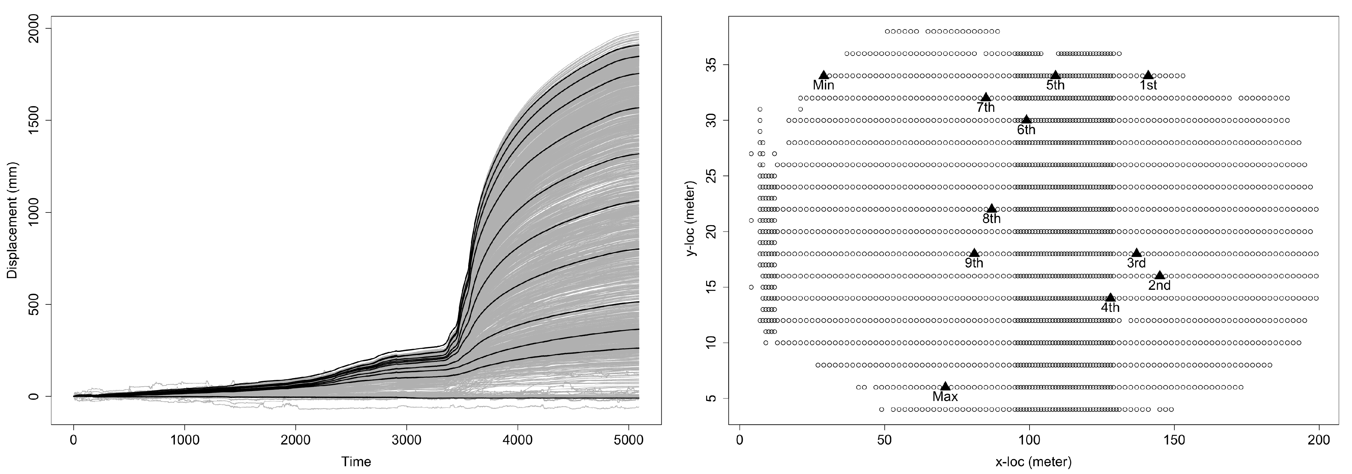
4. The EDQ Technique for Vector Time Series Dimension Reduction

For a k × 1 vector time series { z t = ( z 1 t , , z k t ) , t = 1 , , T } , which is equivalently a set of k scalar time series where k can be large, we want to choose a small subset of those k series to describe { z t = ( z 1 t , , z k t ) , t = 1 , , T } without compromising its overall temporal dynamics, so that information drawn from this small subset is representative of { z t = ( z 1 t , , z k t ) , t = 1 , , T } and also efficient. This can be achieved by using the empirical dynamic quantiles (EDQ) technique introduced by [6]. Given a probability value p [ 0 , 1 ] , the level-p EDQ series of { z t = ( z 1 t , , z k t ) , t = 1 , , T } is defined as
q ( p ) { q t ( p ) , t = 1 , , T } : = arg min q = { q 1 , , q T } C k t = 1 T p z i t q t | z i t q t | + ( 1 p ) z i t q t | z i t q t |
where C k = { { z i t , t = 1 , , T } , i = 1 , , k } is the set of k scalar time series in { z t = ( z 1 t , , z k t ) , t = 1 , , T } . Note that the level p empirical quantile of { z i t , i = 1 , , k } for fixed t is
q t * ( p ) = arg min q R p z i t q | z i t q | + ( 1 p ) z i t q | z i t q | ,
and q t * ( p ) is not necessarily equal to q t ( p ) for any t. Specifically, { q t ( p ) , t = 1 , , T } is one of the k scalar time series in { z t = ( z 1 t , , z k t ) , t = 1 , , T } , and { q t * ( p ) , t = 1 , , T } is not necessarily one. Hence, an EDQ series keeps the temporal dynamics in { z t = ( z 1 t , , z k t ) , t = 1 , , T } , and { q t * ( p ) , t = 1 , , T } does not. Let Q t ( p ) be the level p population quantile corresponding to q t * ( p ) . It is shown in [6] that
lim k Pr t = 1 T | q t ( p ) Q t ( p ) | < ε = 1   for   any   ε > 0   and   given   T .
In practice, we use the EDQ technique to find a quantile level for each of the k time series in { z t = ( z 1 t , , z k t ) , t = 1 , , T } or equivalently C k . Then we choose a small number, say, m = 11 , of them to construct m EDQ series q ( P m ) = { ( q t ( p 1 ) , , q t ( p m ) ) , t = 1 , , T } , with the associated quantile levels 0 p 1 < p 2 < < p m 1 . Now the aforementioned statistical inference made on { z t , t = 1 , , T } can be made to the m EDQ series q ( P m ) in the same way, which will return the same type of estimation and forecast results. In addition, the results obtained from the m EDQ series can be used to draw estimations and forecasts for any other scalar time series in { z t , t = 1 , , T } or C k . For example, for each such scalar time series, we can find its quantile level, say, p . This determines two of the m EDQ series of levels, say, p j and p j , which are the two closest to p . Then forecasts for the level p quantile series can be obtained through interpolating the forecasts for the level p j and p j EDQ series.

5. Applying the ECC–VAR–EDQ Method to Analyze the InSAR Landslide Data

The InSAR landslide data shown in Figure 1 contain 1803 time series observed at 1803 min areas (each of size 4 m 2 ) in a slope of 200 m long and 40 m high, and each time series consists of 5090 cumulative displacement observations, recorded once every 6 min from 31 May to 21 June. As found in Section 2, the actual landslide occurred at around t = 3568 (13:02, 15 June), preceded by a precursory slope deformation at around t = 1600 (4:41, 7 June); and t = 3820 (14:39, 16 June) is well after the landslide. Since an important objective of this analysis is to assess the forecasting capability of the ECC–VAR–EDQ method, we will use the data from t = 1 to t = 1600 as the training sample for parameter estimation and model fitting, then use the fitted model to forecast at t = 1601 to t = 3820 . Since 1803 is a very high number of dimensions, we reduced the dimensions using the EDQ technique, by which and the training sample 11 EDQ series at levels P ( 11 ) = ( Min , 0.1 , 0.2 , 0.3 , 0.4 , 0.5 , 0.6 , 0.7 , 0.8 , 0.9 , Max ) , with Min = 1 / 1803 and Max = 1802 / 1803 , were determined together with their locations. These 11 EDQ series (extended to include data at all 5090 time stamps) and their locations in the slope are displayed in Figure 1 in black, and Table 1.
It was confirmed that some of the 11 EDQ series are non-stationary, which is attributed to either unit root or inside unit-circle roots of the determinant Equation (3). The type of non-stationarity attributed to the inside unit-circle roots is also referred to as the explosive non-stationarity; cf. [15]. To simplify the analysis, we took logarithm transformation on the 11 EDQ time series to remove the explosive non-stationarity as much as possible. That is, define
z i t = log x i t min i , t ( x i t ) + 0.5 , i = 1 , , 11 ; t = 1 , , 5090
where x i t is the original cumulative displacement observation at time t and area (pixel) i corresponding to the 11 quantile levels P ( 11 ) . The 11 EDQ series defined in (11) are displayed in Figure 2. We used as the training sample the 11 EDQ series { z t = ( z 1 , t , , z 11 , t ) , t = 1 , , 1600 } to perform statistical analysis by the ECC–VAR–EDQ method in the sequel.

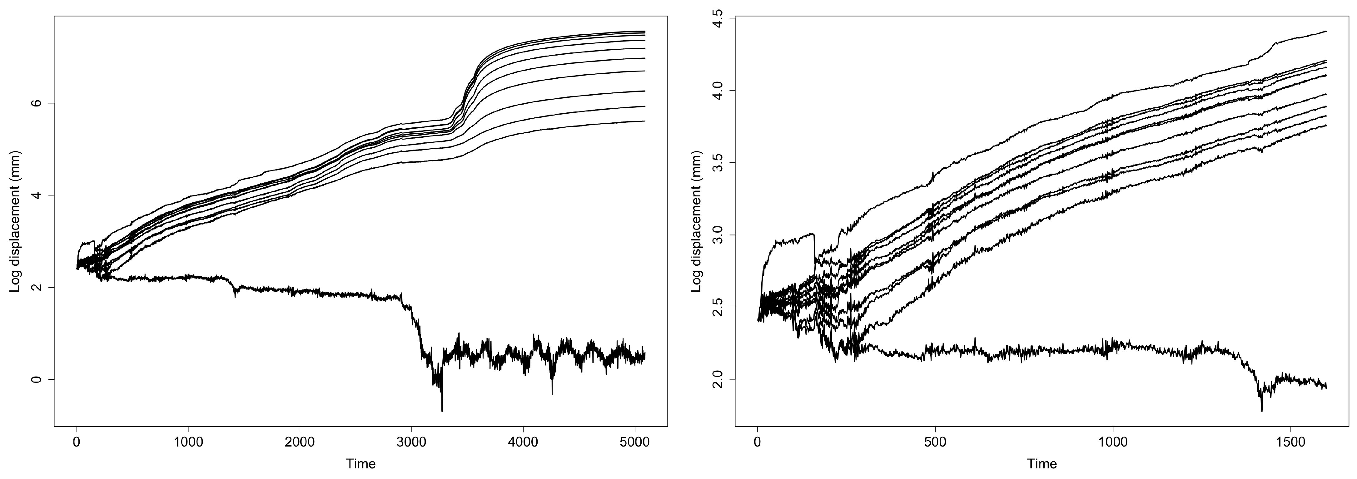
5.1. Unit Root Test and Cointegration Test for the EDQ Series

First, we ran the augmented Dickey–Fuller (ADF) unit root test for the 11 EDQ series { z t = ( z 1 , t , , z 11 , t ) , t = 1 , , 1600 } and their first-order differences { Δ z t } to see whether they each are stationary or not. The level 1%, 5% and 10% critical values of the ADF test statistic, obtainable from the R package urca, are 3.43 , 2.86 and 2.57 , respectively. By the ADF test, the null hypothesis of unit root non-stationarity should be rejected at a significance level if the absolute value of the computed ADF statistic is greater than the absolute value of the corresponding critical value. The ADF unit test results for the 22 times series in { z t } and { Δ z t } are provided in Table 2, from which we see statistical evidence, at the 1% or 5% significance level, of stationarity for 16 series, and there is no significant evidence to reject the unit-root non-stationarity for the level-( Min , 0.6 , 0.7 , 0.8 , 0.9 , Max ) EDQ series in { z t } .
Next, we used ca.jo() to perform a sequence of cointegration tests based on the trace statistic for the vector time series { z t } determined by the 11 EDQ series. The null hypothesis of r = rank ( Π ) r 0 was to be rejected at significance level α if the trace statistic was greater than the level α critical value. The cointegration test results for r 0 = 0 to 10 are provided in Table 3.
Table 3 suggests the best estimate of the cointegration rank is r ^ = 6 . Using ca.jo(), the CCA based estimate of the cointegration vectors β , with its top 6 rows constituting a 6 × 6 identity matrix, is found to be
β ^ = 1 0 0 0 0 1 177.6742 36.5351 25.6465 21.2280 8.0301 15.0115 397.0240 62.0006 44.8457 36.3807 13.7202 26.0822 538.0373 103.0722 63.2254 51.6327 12.8647 42.5018 635.1576 109.8483 71.2795 57.6532 16.9223 46.6249 125.5005 20.1797 12.3700 10.3835 2.6405 8.1719

5.2. Estimating and Fitting the ECC(r)–VAR(p) Model for the EDQ Series

Given r ^ = 6 and c ( t ) = c 0 , we still need an estimate of p before we can fit the ECC( r ^ )-VAR(p) model (6) by fitting the multivariate linear regression model (7) using the least squares method. Instead of using a model selection criterion, we used the coefficient of determination R 2 given by (9) to assess the adequacy of the model. Accordingly, p = 2 was found to be adequate with R 2 = 0.99 based on the associated multivariate linear regression analysis. Then we used the R function cajorls() to fit an ECC(6)-VAR(2) model for the 11 EDQ series { z t } shown in the right panel in Figure 2, giving the following results:
Δ z ^ t = α ^ y t 1 + Φ ^ 1 * Δ z t 1 + c ^ 0 , where
α ^ = 0.0029 0.1037 0.1410 0.0772 0.2227 0.0291 0.0008 0.0694 0.0814 0.0581 0.1458 0.0298 0.0000 0.0059 0.0739 0.0075 0.0859 0.0586 0.0002 0.0099 0.0140 0.0060 0.0364 0.0368 0.0000 0.0031 0.0222 0.0067 0.0306 0.0219 0.0009 0.0379 0.0697 0.0285 0.1006 0.0049 0.0011 0.0106 0.0151 0.0138 0.0206 0.0077 0.0011 0.0218 0.0448 0.0181 0.0612 0.0026 0.0001 0.0082 0.0102 0.0156 0.0192 0.0076 0.0000 0.0112 0.0283 0.0055 0.0552 0.0048 0.0009 0.0079 0.0069 0.0081 0.0206 0.0174 ,
Φ ^ 1 * = 0.409 0.022 0.067 0.227 0.626 0.378 0.666 0.156 0.323 0.783 0.304 0.001 0.632 0.056 0.171 0.370 0.174 0.711 0.303 0.165 0.567 0.244 0.002 0.037 0.458 0.091 0.174 0.051 0.079 0.076 0.020 0.272 0.133 0.001 0.000 0.062 0.457 0.106 0.169 0.127 0.138 0.064 0.065 0.176 0.001 0.027 0.051 0.152 0.612 0.014 0.084 0.031 0.002 0.281 0.129 0.001 0.143 0.050 0.129 0.332 0.353 0.437 0.154 0.113 0.523 0.274 0.001 0.087 0.026 0.163 0.160 0.007 0.169 0.010 0.157 0.343 0.269 0.001 0.134 0.069 0.144 0.213 0.035 0.346 0.466 0.145 0.497 0.304 0.000 0.079 0.069 0.154 0.232 0.123 0.102 0.043 0.601 0.296 0.329 0.001 0.003 0.019 0.214 0.074 0.038 0.065 0.106 0.167 0.124 0.013 0.001 0.237 0.082 0.066 0.357 0.249 0.077 0.041 0.051 0.037 0.160
and c ^ 0 = ( 0.008 , 0.0068 , 0.0074 , 0.003 , 0.0016 , 0.011 , 0.0085 , 0.0103 , 0.0014 , 0.0003 , 0.0063 ) .

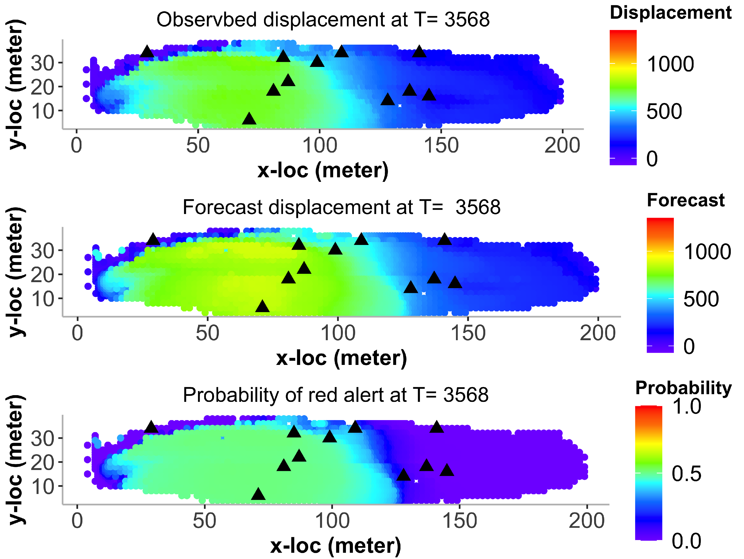
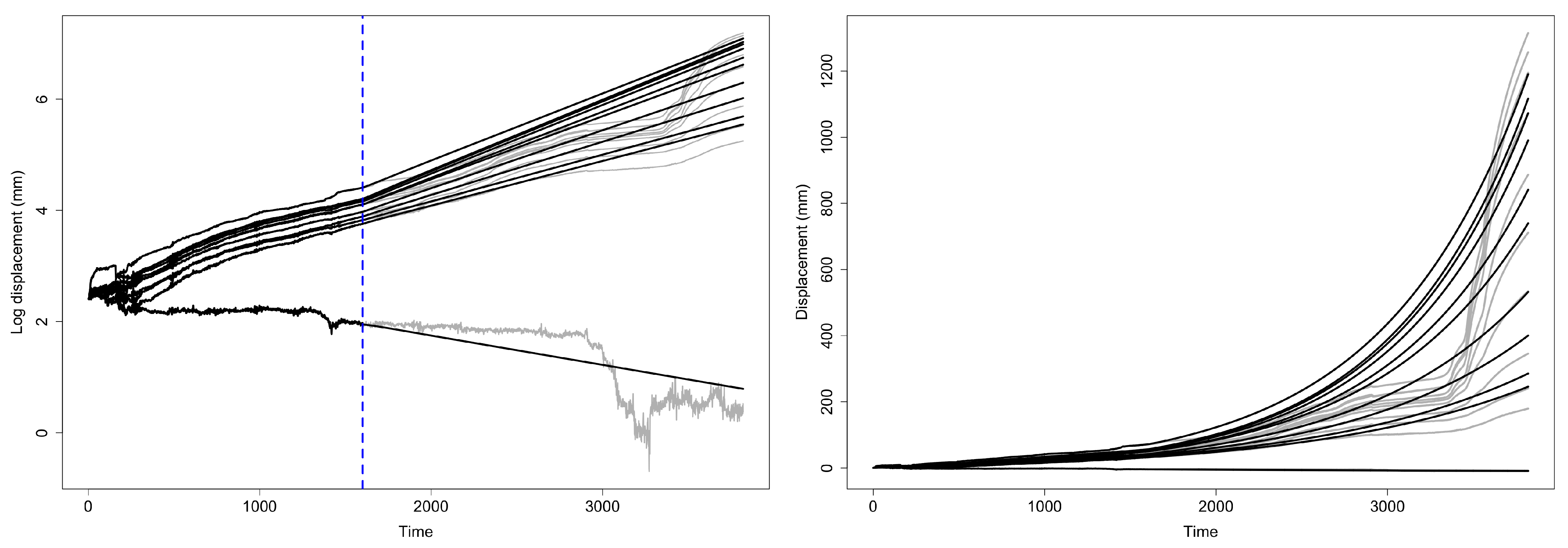
5.3. Landslide Displacement Forecasting

Based on the fitted ECC(6)-VAR(2) model for the 11 EDQ series, we could obtain the forecasts of Δ z t and z t for t = 1601 until t = 3820 , i.e., those time states in the test sample. Equation (10) was used for all calculations. The forecasts of the displacement and velocity were then calculated by the formulas x i , T + h ^ = e z i , T + h ^ + min i , t ( x i t ) 0.5 and Δ x i , T + h ^ = x i , T + h ^ x i , T + h 1 ^ , respectively. These forecasts are plotted in Figure 3.

6. Probabilistic Landslide Prediction via the ECC–VAR–EDQ Method

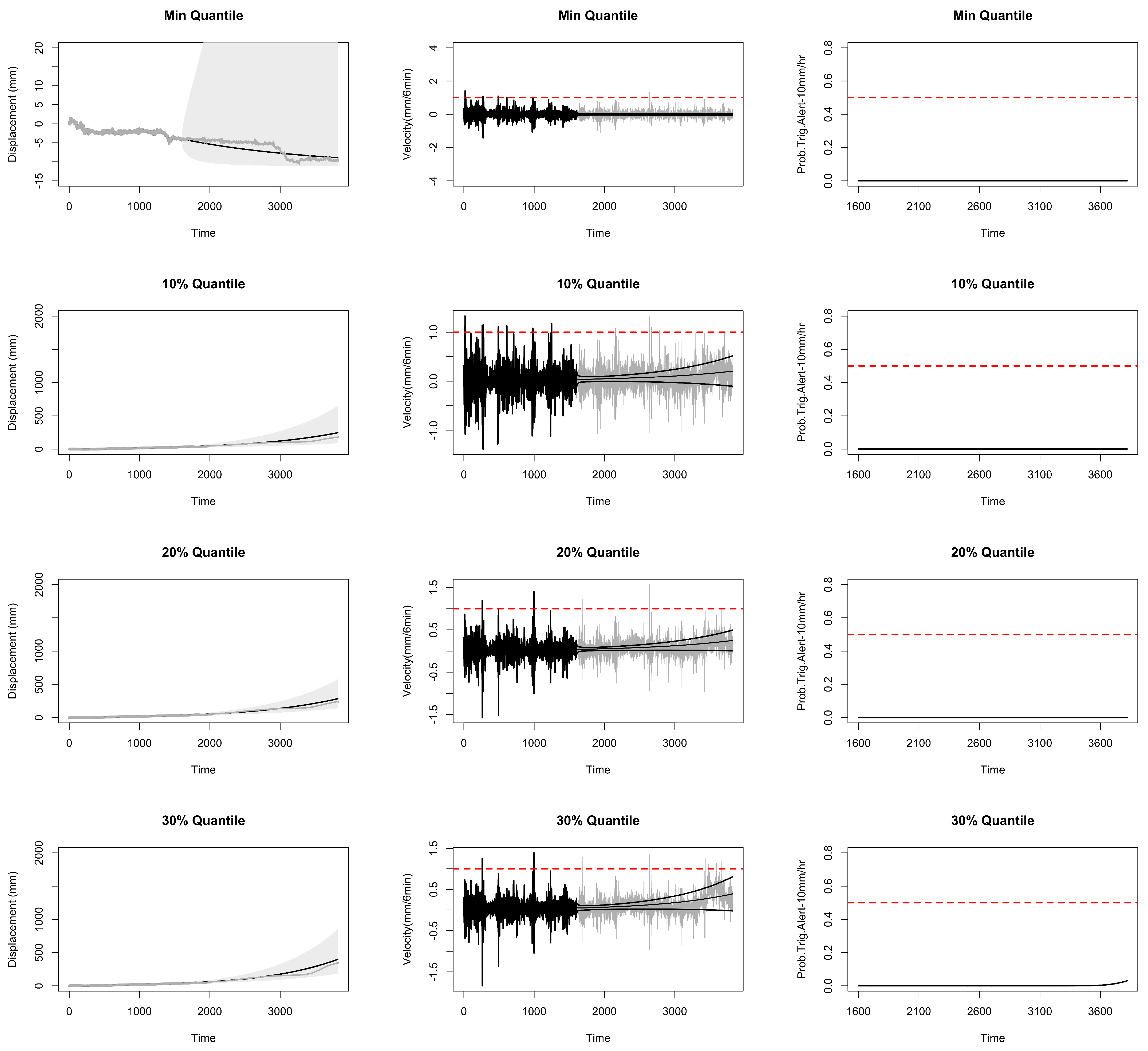
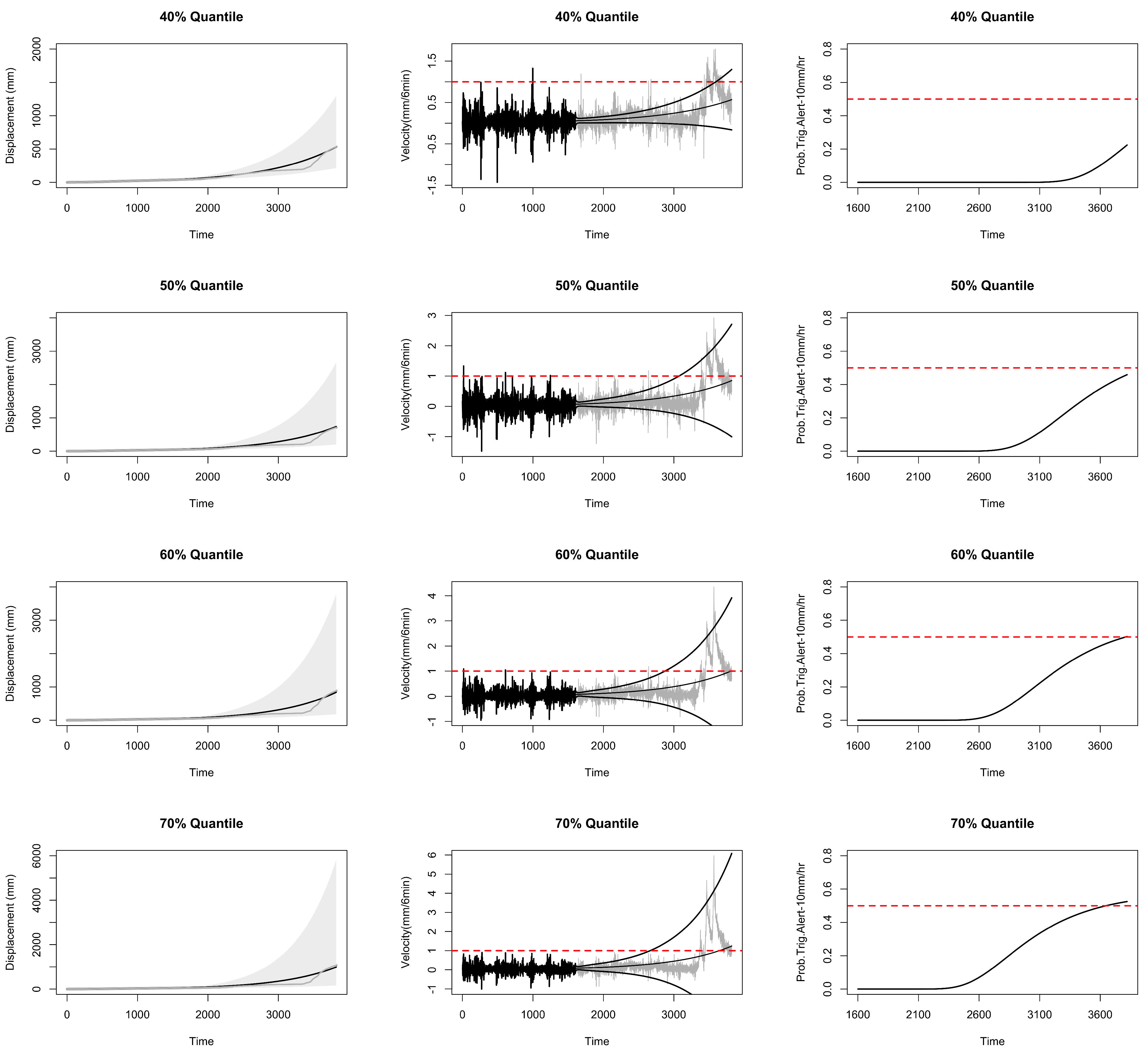
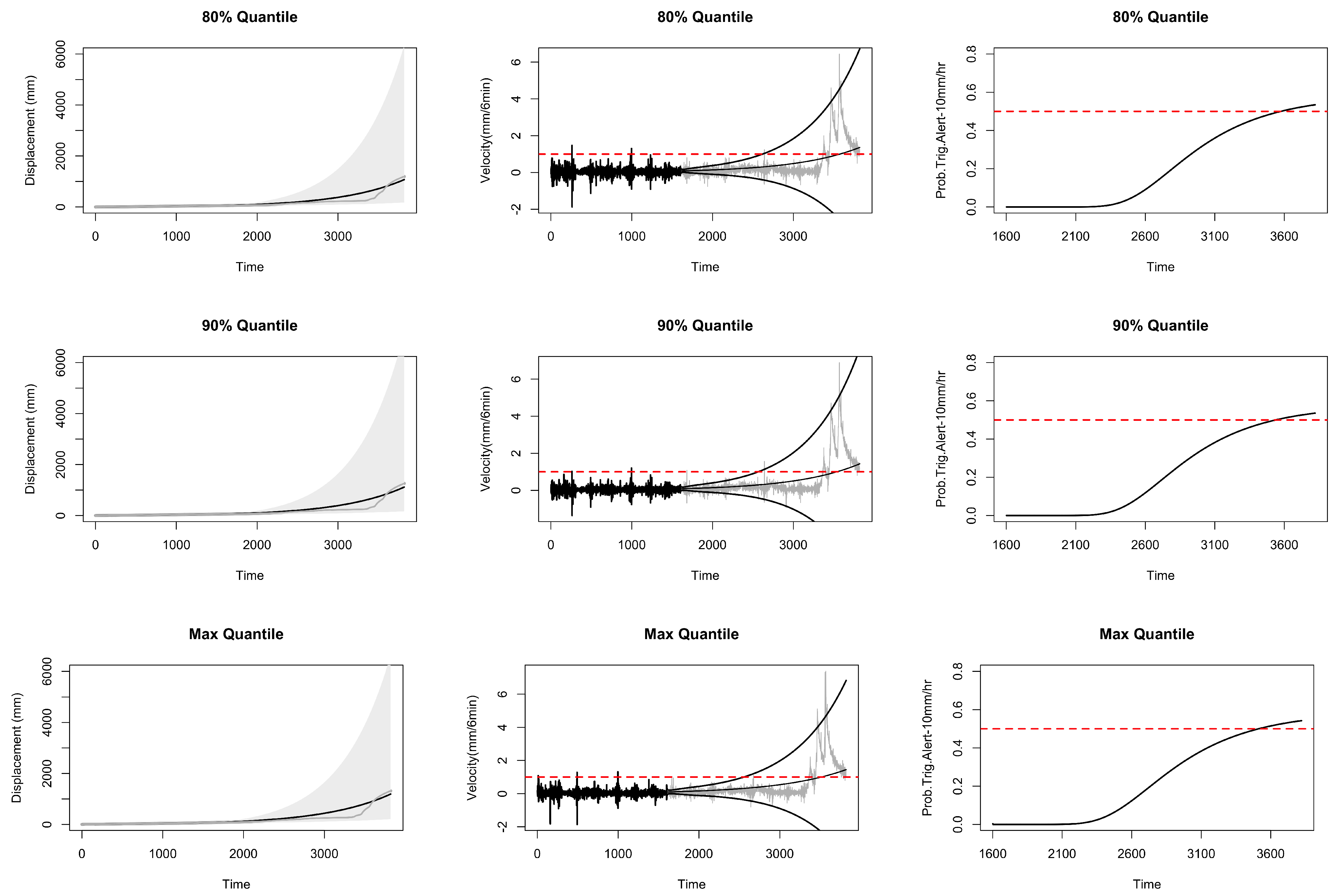
6.1. Forecast Intervals for Displacement and Velocity

In order to see the variations in the forecasts x i , T + h ^ and Δ x i , T + h ^ , we resorted to find the corresponding forecast intervals. This required finding the variances of x i , T + h ^ and Δ x i , T + h ^ first, which can be achieved by applying the δ -method or an empirical sampling plug-in method based on the forecasts Δ z i , T + h ^ and z i , T + h ^ and their variance and covariance matrices. In fact, each component in these variance and covariance matrices could be estimated from the predicted values of Δ z t and z t , with t = T + 1 , , T + h , by fitting the multivariate linear regression model (7). For simplicity of presentation, we use Var ( Δ z i t ^ ) and Var ( z i t ^ ) to denote the estimated variances of Δ z i t ^ and z i t ^ , respectively. By asymptotic normal approximation for GLS estimators, an approximately 80% forecast interval for Δ z i t is given as
Δ z i t ^ 1.28 Var ( Δ z i t ^ ) , Δ z i t ^ + 1.28 Var ( Δ z i t ^ ) , t = T + 1 , , T + h ,
where 1.28 is the value of 0.9 quantile of standard normal distribution Φ 1 ( 0.9 ) 1.28 . Furthermore, an approximately 80% forecast interval for z i t is given as
z i t ^ 1.28 Var ( z i t ^ ) , z i t ^ + 1.28 Var ( z i t ^ ) , t = T + 1 , , T + h ,
Results from (13) and (14) can be used to find 80% forecast intervals for x i t = e z i t + min i , t ( x i t ) 0.5 by either the δ -method or transformation. As an example, let us find an approximately 80% forecast interval for x i , T + 1 . By the δ -method,
E ( x i , T + 1 ^ ) e z i , T e E ( Δ z i , T + 1 ^ ) + min i , t ( x i t ) 0.5 e z i , T + 1 ^ + min i , t ( x i t ) 0.5 = x i , T + 1 ^
Var ( x i , T + 1 ^ ) e 2 z i , T + 2 E ( Δ z i , T + 1 ^ ) Var ( Δ z i , T + 1 ^ ) e 2 z i , T + 1 ^ Var ( Δ z i , T + 1 ^ )
Therefore, using (15) and (16), an approximately 80% forecast interval for the cumulative displacement x i , T + 1 can be computed from
x i , T + 1 ^ 1.28 Var ( x i , T + 1 ^ ) , x i , T + 1 ^ + 1.28 Var ( x i , T + 1 ^ ) .
Similarly to (15) and (16), we can get
E ( x i , T + h ^ ) x i , T + h ^ , and Var ( x i , T + h ^ ) e 2 z i , T + h ^ Var ( Δ z i , T + h ^ ) ,
from which we can compute an approximately 80% forecast interval for x i , T + h . However, the approximation error involved in estimating Var ( x i , T + h ^ ) may be excessive so as to render the interval inaccurate. We propose to compute an approximately 80% forecast interval for x i , T + h based on a monotonic transformation of that for the log-displacement z i , T + h . Namely, the referenced 80% forecast interval for x i , T + h is
e z i , T + h ^ 1.28 Var ( z i , T + h ^ ) + min i , t ( x i t ) 0.5 , e z i , T + h ^ + 1.28 Var ( z i , T + h ^ ) + min i , t ( x i t ) 0.5 .
Results from (13) and (14) can also be used to find 80% forecast intervals for velocity v i , T + h = Δ x i , T + h at location i and time t = T + 1 , , T + h , . To achieve this, we first applied the δ -method to find an estimated variance of v i , T + h ^ = Δ x i , T + h ^ , which is
Var ( v i , T + h ^ ) = Var ( x i , T + h ^ ) + Var ( x i , T + h 1 ^ ) 2 Cov x i , T + h ^ , x i , T + h 1 ^ e z i , T + h ^ e z i , T + h ^ e z i , T + h 1 ^ Var ( Δ z i , T + h ^ ) + e z i , T + h 1 ^ e z i , T + h 1 ^ e z i , T + h ^ Var ( Δ z i , T + h 1 ^ ) e z i , T + h ^ + z i , T + h 1 ^ Cov Δ z i , T + h ^ , Δ z i , T + h 1 ^ .
Then, a normal approximation based 80% forecast interval for v i , T + h ^ is
v i , T + h ^ 1.28 Var ( v i , T + h ^ ) , v i , T + h ^ + 1.28 Var ( v i , T + h ^ ) .
Alternatively, an approximately 80% forecast interval for v i , T + h = x i , T + h x i , T + h 1 can be obtained by transforming that for x i , T + h and x i , T + h 1 as follows:
e z i , T + h ^ 1.28 Var ( z i , T + h ^ ) e z i , T + h 1 ^ + 1.28 Var ( z i , T + h 1 ^ ) , e z i , T + h ^ + 1.28 Var ( z i , T + h ^ ) e z i , T + h 1 ^ 1.28 Var ( z i , T + h 1 ^ ) .
Results of the forecasts and approximately 80% forecast intervals for the 11 EDQ series of cumulative displacement x i t and velocity v i t for t from 1601 to 3820 are displayed in the first two columns of Figure 4, Figure 5 and Figure 6. A horizontal line indicating the red-alert velocity of 10mm/hr is added to each velocity plot there.

6.2. Probability of Future Risk of Landslide

Forecasts of the displacement and velocity and their respective 80% forecast intervals plotted in Figure 4, Figure 5 and Figure 6 show that they correctly capture the overall trends of ground movement in terms of displacement and velocity. However, they also show the need for improving the forecasting accuracy, and it is difficult to interpret these results for the general public. On the other hand, interpreting the risk of an incoming landslide in terms of a probability is much more accessible to general public. Hence, we propose to measure this risk by a probability of the forecast ground motion velocity exceeding a red-alert level. The risk may be alternatively evaluated by comparing the forecast displacement with a red-alert displacement level, but it will not be pursued here due to lack of consensus about setting the red-alert displacement level.
In field of slope failure research, it is commonly accepted that a ground motion velocity of 10 mm per hour or 1 mm per 6 min is an alarming number indicating slope failure. Since the cumulative displacement in our InSAR data is updated roughly every 6 min, the referenced velocity v i t is actually the change of displacement per 6 min. Therefore, we will compute the probability of v i t exceeding 1 at location i and t = T + 1 , , T + h , . Calculating this probability requires at least an approximate probability distribution for v i t be available. By the asymptotic properties of the GLS estimation in multivariate linear regression and the δ -method, it can be shown that
v i t a s y m . N ( v i t ^ , Var ( v i t ^ ) ) , equivalently v i t v i t ^ Var ( v i t ^ ) a s y m . N ( 0 , 1 )
where Var ( v i t ^ ) is given in Equation (18). Now the probability of the velocity v i t exceeding the red-alert threshold level is
Pr ( v i t 1 ) 1 Φ 1 v i t ^ Var ( v i t ^ ) , i = 1 , , k ; t = T + 1 , , T + h ,
Calculated values of Pr ( v i t 1 ) for the 11 EDQ series at t from 1601 to 3820 are displayed in the right panels of Figure 4, Figure 5 and Figure 6.
The probability plots in Figure 4, Figure 5 and Figure 6 provide very accurate probability forecasting on the impending landslide. For example, Pr ( v 11 , t 1 ) > 0.5 for the level Max EDQ series when t 3513 , 5.5 h ahead of the actual landslide occurred around t = 3568 ; and Pr ( v 10 , t 1 ) > 0.5 for the level-0.9 EDQ series when t 3575 , within 42 min after the actual landslide. Recalling that these forecast and probability results are computed using the observations at t from 1 to 1600, about 196.8 h before the actual landslide. Therefore, we can conclude that our ECC–VAR–EDQ method is able to accurately predict an impending landslide, with greater than 50% red-alert probability, more than 196 h in advance.

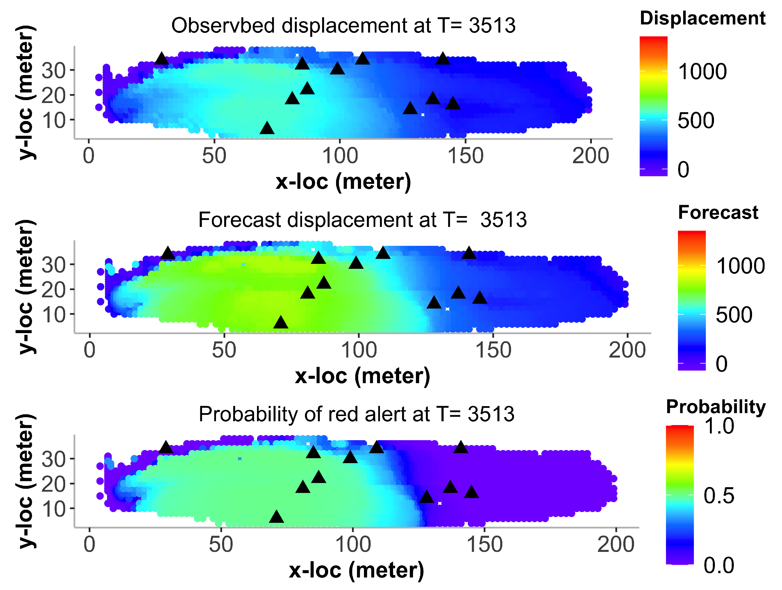
6.3. Landslide Prediction for All Locations

In addition to getting the probabilistic forecasting results for the 11 EDQ series, we used the ECC–VAR–EDQ method to compute the displacement forecasts x i t , the velocity forecasts v i t and the forecast probabilities Pr ( v i t 1 ) for all 1803 locations and at time t from 1601 to 3820. The key method used is interpolation. For example, for a location with EDQ level 0.83, all the forecasts at this location were calculated as the weighted average of those at level 0.8 and level 0.9 EDQ locations. Namely, for t = 1601 to 3820
x ( 0.83 ) , t ^ = 0.7 · x ( 0.8 ) , t ^ + 0.3 · x ( 0.9 ) , t ^ v ( 0.83 ) , t ^ = 0.7 · v ( 0.8 ) , t ^ + 0.3 · v ( 0.9 ) , t ^ Pr ( v ( 0.83 ) , t 1 ) = 0.7 · Pr ( v ( 0.8 ) , t 1 ) + 0.3 · Pr ( v ( 0.9 ) , t 1 )
An mp4 video mine_r6.mp4 is provided in Supplementary Materials which displays the aforementioned forecasts of displacement and the red-alert probability for all 1803 locations and at time t from 1601 to 3820. Two screenshots of this video at time t = 3513 and 3568 are shown in Figure 7 and Figure 8, respectively. The video and the screenshot show that the displacement forecasts capture the spatiotemporal dynamics and trends of the actual slope surface movement at all locations very well, and the red-alert probability forecasts provide timely predictions of the landslides at all locations.

7. Conclusions

We have developed an ECC–VAR–EDQ method to characterize and analyze high-dimensional, unit-root non-stationary vector time series. The model underpinning the new method has a vector autoregression form with an error-correction cointegration representation. We showed how to use the new method to make statistical inferences, including parameter estimation, goodness of model fit test, forecasts and forecast intervals, for high-dimensional non-stationary vector time series data. An advantage of our method is that we can use a small number of EDQ series to reduce the dimension and apply an ECC–VAR model to these EDQ series. Thus, the procedure is computationally feasible, with negligible loss of spatial-temporal information of the data.
We inferred an ECC(6)–VAR(2)–EDQ(11) model to analyze the InSAR landslide data observed at 1803 locations and across 5090 time states. The statistical inference results were shown to be remarkably informative. For example, the goodness of fit statistic R 2 = 0.99 was close to 1. The results also estimated 80% forecast intervals that can be used to calculate the probability of a possible red-alert event in the future based on the up-to-date observations. Once this probability is higher than 50%, we can raise an early warning alert about a probable incoming landslide. For the motivational landslide case study in this paper, the results by our method can predict the incoming landslide more than 8 days in advance, which means we will have enough time to prepare an effective mitigation plan and reduce the damage caused by landslides.
Although our ECC–VAR–EDQ method has a capability for timely forecasting an incoming landslide, there is still room for improvement. For example, the ECC approach is only able to deal with the unit-root non-stationary vector time-series, but the real data can be non-stationary of other types. To enable using ECC, we took a logarithm transform to our original data, but we still found there are some sharp increases (diffusion) in those high level quantile series, suggesting the log-transformation is successful but not ideal. Hence in future work, we will investigate improving ECC to handle other types of non-stationarity in high-dimensional VAR time series.
Finally, note that most of the current landslide monitoring and forecast research are not configured for computational scalability and as such has focused on only uni-variate time series or low-dimensional vector time series; cf. [3]. Thus, their methods are not able to handle spatial dependence and temporal dynamics jointly for InSAR landslide data. Our ECC–VAR–EDQ method is able to effectively handle this spatial dependence and temporal dynamics simultaneously in a computationally feasible way.

Supplementary Materials

The following are available online at https://www.mdpi.com/article/10.3390/forecast3040051/s1.

Author Contributions

Conceptualization, G.Q. and A.T.; methodology, G.Q.; software, H.Z.; validation, G.Q., A.T. and H.Z.; formal analysis, G.Q. and H.Z.; investigation, H.Z.; data curation, A.T.; writing—original draft preparation, H.Z.; writing—review and editing, G.Q.; visualization, H.Z.; supervision, G.Q. and A.T.; funding acquisition, A.T. All authors have read and agreed to the published version of the manuscript.

Funding

This research was partly funded by the U.S. DoD High Performance Computing Modernization Program (HPCMP) and RDECOM International Technology Center-Pacific (ITC-PAC) contract number: FA5209-18-C-0002.

Acknowledgments

The authors thank the Assistant Editor and the four anonymous reviewers for providing valuable comments and suggestions, leading to an improvement of the presentation of the paper.

Conflicts of Interest

The authors declare no conflict of interest.

References

  1. Dick, G.J.; Eberhardt, E.; Cabrejo-Liévano, A.G.; Stead, D.; Rose, N.D. Development of an early-warning time-of-failure analysis methodology for open-pit mine slopes utilizing ground-based slope stability radar monitoring data. Can. Geotech. J. 2014, 52, 515–529. [Google Scholar] [CrossRef]
  2. Glade, T.; Crozier, M.J. Landslide Hazard and Risk-Concluding Comment and Perspectives. In Landslide Hazard and Risk; John Wiley & Sons, Ltd.: Hoboken, NJ, USA, 2012; Chapter 26; pp. 765–774. [Google Scholar] [CrossRef]
  3. Intrieri, E.; Carlá, T.; Gigli, G. Forecasting the time of failure of landslides at slope-scale: A literature review. Earth-Sci. Rev. 2019, 193, 333–349. [Google Scholar] [CrossRef]
  4. Wang, H.; Qian, G.; Tordesillas, A. Modeling big spatio-temporal geo-hazards data for forecasting by error-correction cointegration and dimension-reduction. Spat. Stat. 2020, 36, 100432. [Google Scholar] [CrossRef]
  5. Tsay, R.S. Multivariate Time Series Analysis: With R and Financial Applications; John Wiley & Sons: Hoboken, NJ, USA, 2014. [Google Scholar]
  6. Peña, D.; Tsay, R.S.; Zamar, R. Empirical dynamic quantiles for visualization of high-dimensional time series. Technometrics 2019, 61, 429–444. [Google Scholar] [CrossRef]
  7. Wessels, S.D.N. Monitoring and Management of a Large Open Pit Failure. Ph.D. Thesis, University of the Witwatersrand, Johannesburg, South Africa, 2009. [Google Scholar]
  8. Harries, N.; Noon, D.; Rowley, K. Case studies of slope stability radar used in open cut mines. In Stability of Rock Slopes in Open Pit Mining and Civil Engineering Situations; SAIMM Johannesburg: South Africa, 2006; pp. 335–342. [Google Scholar]
  9. Casagli, N.; Catani, F.; Del Ventisette, C.; Luzi, G. Monitoring, prediction, and early warning using ground-based radar interferometry. Landslides 2010, 7, 291–301. [Google Scholar] [CrossRef]
  10. Stacey, T. Stability of Rock Slopes in Open Pit Mining and Civil Engineering Situations; The South African Institute of Mining and Metallurgy: Johannesburg, South Africa, 2006. [Google Scholar]
  11. Kwiatkowski, D.; Phillips, P.C.; Schmidt, P.; Shin, Y. Testing the null hypothesis of stationarity against the alternative of a unit root: How sure are we that economic time series have a unit root? J. Econom. 1992, 54, 159–178. [Google Scholar] [CrossRef]
  12. Pfaff, B. Analysis of Integrated and Cointegrated Time Series with R; Springer Science & Business Media: Berlin/Heidelberg, Germany, 2008. [Google Scholar]
  13. Johansen, S. Statistical analysis of cointegration vectors. J. Econ. Dyn. Control 1988, 12, 231–254. [Google Scholar] [CrossRef]
  14. Johansen, S.; Juselius, K. Maximum likelihood estimation and inference on cointegration—With applications to the demand for money. Oxf. B Econ. Stat. 1990, 52, 169–210. [Google Scholar] [CrossRef]
  15. Phillips, P.C.; Wu, Y.; Yu, J. Explosive behavior in the 1990s Nasdaq: When did exuberance escalate asset values? Int. Econ. Rev. 2011, 52, 201–226. [Google Scholar] [CrossRef] [Green Version]
Figure 1. (Left) Slope surface displacement from 31 May to 21 June with 1083 × 5090 observations in total. (Right) The 1803 small areas (locations). The 11 locations highlighted in black correspond to the 11 EDQ series at quantile levels 0.0 (min), 0.1, ⋯, 0.9 and 1.0 (maximum).
Forecasting 03 00051 g001
Figure 2. (Left) The 11 log-displacement EDQ series from t = 1 to t = 5090. (Right) The 11 log-displacement EDQ series from the training sample t = 1 to t = 1600.
Forecasting 03 00051 g002
Figure 3. (Left) Log-displacements of the 11 selected EDQ series from t = 1 to t = 3820 . (Right) Displacements of the 11 selected EDQ series from t = 1 to t = 3820 . The black lines represent the forecasts and the gray lines represent the actual observations.
Forecasting 03 00051 g003
Figure 4. Slope surface displacement (Left), velocity (Middle) and probability of triggering a red alert (Right) in the Min, 10%, 20% and 30% EDQ series. The forecast displacement and velocity are plotted in black with their estimated 80% forecast intervals, and the corresponding observed data are plotted in gray lines. The red dashed line in each velocity plot is the velocity alert threshold, which is 1 mm/6 min (10 mm/h), and indicates 50% probability of triggering a red alert in the probability plots.
Forecasting 03 00051 g004
Figure 5. Slope surface displacement (Left), velocity (Middle) and probability of triggering red alert (Right) for the 40%, 50%, 60% and 70% EDQ series. The forecast displacement and velocity are plotted in black with their estimated 80% forecast intervals, and the corresponding observed data are plotted in gray lines. The red dashed line in each velocity plot is the velocity alert threshold, which is 1 mm/6 min (10 mm/h), and indicates 50% probability of triggering a red alert in the probability plots.
Forecasting 03 00051 g005
Figure 6. Slope surface displacement (Left), velocity (Middle) & probability of triggering red alert (Right) for the 80%, 90% & Max EDQ series. The forecast displacement and velocity are plotted in black with their estimated 80% forecast intervals, and the corresponding observed data are plotted in gray lines. The red dashed line in each velocity plot is the velocity alert threshold, which is 1 mm/6 min (10 mm/h), and indicates 50% probability of triggering a red alert in the probability plots.
Forecasting 03 00051 g006
Figure 7. Screenshot of mine_r6.mp4 at time t = 3513. The top (middle) panel displays the actual (forecast) displacement, and the bottom panel displays the probability forecasts at all locations. The ▴s indicate the 11 EDQ locations. Results were obtained based on the data at t = 1 , , 1600 .
Forecasting 03 00051 g007
Figure 8. Screenshot of mine_r6.mp4 at time t = 3568. The top (middle) panel displays the actual (forecast) displacement, and the bottom panel displays the probability forecasts at all locations. The ▴s indicate the 11 EDQ locations. Results were obtained based on the data at t = 1 , , 1600 .
Forecasting 03 00051 g008
Table 1. Positions (pixels), in 1 to 1803, of the selected 11 EDQ time series.
Quantile LevelSelected PixelQuantile LevelSelected Pixel
Min2020.6827
0.114320.7672
0.214540.8685
0.313920.9630
0.41307Max534
0.5995
Table 2. Unit root test results for the level/first-order difference of the 11 selected EDQ time series (log transformed). Superscript *** indicates rejecting the null hypothesis at 1 % level; ** indicates rejecting the null hypothesis at 5 % level. All these tests were conducted by including a trend term and up to 13 lags.
Quantile Level pPixel IDAugment Dickey−Fuller(ADF)
Min202−0.9334/−26.8762 ***
0.11432−2.9837 **/−21.3401 ***
0.21454−4.6048 ***/−21.5254 ***
0.31392−3.1837 **/−17.0134 ***
0.41307−3.3355 **/−17.7037 ***
0.5995−2.8695 **/−16.1240 ***
0.6827−1.7187/−14.2224 ***
0.7672−1.4623/−13.3679 ***
0.8685−1.3172/−13.9375 ***
0.9630−1.5063/−11.7859 ***
Max534−1.3808/−17.9545 ***
Table 3. Null hypotheses, trace statistic and level-(10%, 5%, 1%) critical values of cointegration tests.
HypothesisStatistic10%5%1%
r 10 0.426.508.1811.65
r 9 5.8215.6617.9523.52
r 8 16.7728.7131.5237.22
r 7 35.1945.2348.2855.43
r 6 57.5666.4970.6078.87
r 5 120.1485.1890.39104.20
r 4 253.29118.99124.25136.06
r 3 404.85151.38157.11168.92
r 2 628.63186.54192.84204.79
r 1 998.73226.34232.49246.27
r 0 1869.85269.53277.39292.65
Publisher’s Note: MDPI stays neutral with regard to jurisdictional claims in published maps and institutional affiliations.

