1. Introduction
The energy systems increasingly need demand response for balancing and reduction of environmental impacts such as greenhouse gas emissions. Buildings have excellent demand response potential [
1,
2,
3]. Tapping this potential requires the ability to accurately forecast short-term energy demand, its flexibility, and the load control responses. Accurate modeling and forecasting are essential to utilize a model-based optimal control for demand response and peak demand shaving.
Reviews of building energy modelling for control and operation, by Xiwang and Ji [
4], and by Harish and Kumar [
5], made the following conclusions. First, detailed physical models have high accuracy, but are difficult to utilize in an on-line building operation because they have many parameters and require large computation time and power. Second, statistics and machine learning (ML) models are fast, and their accuracy good enough for model-based control, but these methods require a large amount of training data that covers the building operation range. Third, reducing the computational cost and memory demand for building energy modeling and optimal control, while maintaining the accuracy, is an urgent issue for on-line practical applications.
Based on the analysis above, it would be beneficial to develop methods that combine the best parts of physical and statistical modelling while avoiding their drawbacks. To elaborate, high-detail physical models based in tools such as Modelica [
6], EnergyPlus [
7], and IDA [
8] require a lot of manual work, making it difficult to deploy and utilize them at large scale in a cost-efficient way. This type of physical models are also computationally heavy, and it is therefore difficult to utilize them in model-based optimization. Moreover, their deployment to production use is also a challenge due to the simulation tools used to implement these models. On the other hand, machine learning-based methods are scalable, accurate, and require less human effort in the modelling [
9,
10,
11,
12,
13]. Their deployment is also easier and supported by existing tools and infrastructure [
14,
15,
16]. Machine learning models also typically provide fast enough inference for model-based optimization. Moreover, gradient-based methods such as neural networks make it possible to utilize gradient information and thus converge much faster than gradient-free methods [
17,
18,
19]. However, ML models also have their limitations. They typically require a lot of data to provide good results and even with large amount of training data, it is impossible to cover all situations that need to be forecast [
20]. This makes it risky to utilize machine learning methods as they can produce large errors in exceptional situations.
There are several ways to combine physical-based modelling with machine learning. For example, Koponen et al. [
21] developed and studied combinations of several model hybridization approaches such as residential hybrid, constraining model, and physically based input forecasts. Another typical way to combine physics-based modelling and ML is to utilize a physics-based simulator to generate training data for a ML model [
22,
23,
24,
25,
26,
27,
28]. This is a natural way to combine physics-based modelling and ML, because a main limitation of ML is the lack of training data on all relevant situations. This is especially important in situations where the ML model is used for demand-side management. A common feature of existing studies that use a physics-based simulator for generating training data is that a separate ML model is trained for every building. These type of approaches can combine some of the benefits of physic- and ML-based modelling, but some drawbacks still remain. To elaborate, these types of approaches make it possible to utilize faster and more easily deployable ML models in model-based control, but still require manual work for building modelling. This is because the ML model is only trained for one type of building and it cannot generalize to new buildings. For the same reason, the ML model does not have to learn to approximate the underlying physics encoded into the simulation models, and therefore the model is still not able to perform well in situations not covered by the training data.
To tackle these limitations of the existing work, this paper proposes a novel approach for combining physics-based simulator and ML based modelling. The key idea and main novelty in the proposed approach is that instead of training a separate ML model for each building we use simulated data from a large pool of buildings to train a single Artificial Neural Network (ANN). In this way, the ML models must learn to approximate the physics of the simulation model in order to generalize to new buildings and weather conditions. This approach makes it possible to forecast buildings energy demand just based on building’s characteristics and thus makes it possible to use ML models in situations with no energy consumption data of a specific building. Moreover, the main benefit of the proposed approach is that once the ANN model has been trained, we can completely replace the original simulator. This is important since it makes it possible to have the benefits of ANNs (i.e., ease of deployment, fast inference and gradient-based optimization in model-predictive control) while having the benefits of physics-based models at the same time.
To evaluate the proposed approach, we developed a Feed Forward Neural Network (FFNN) to forecast buildings heat demand based on building characteristics, weather, and temporal data. We used a dynamic hourly based energy model, based on EN ISO 13790:2008 and EN 15241:2007 standards, to generate training, validation, and test data sets. The generated data sets consist of three types of buildings with different parameter combinations for building construction year, dimensions, ventilation heat recovery, and geographical location. The model was evaluated with a test set consisting of a full year of data from 60 buildings (20 from each building type).
The rest of the paper is structured as follows.
Section 2 introduces the novel approach proposed in the paper. It describes the original physical heating and cooling simulator, generated datasets, and the neural network developed for the task.
Section 3 presents the validation and results of the study. In
Section 4, there is discussion about the results and ideas for future work.
Section 5 concludes the paper.
2. Methodology and Approach
2.1. Overview
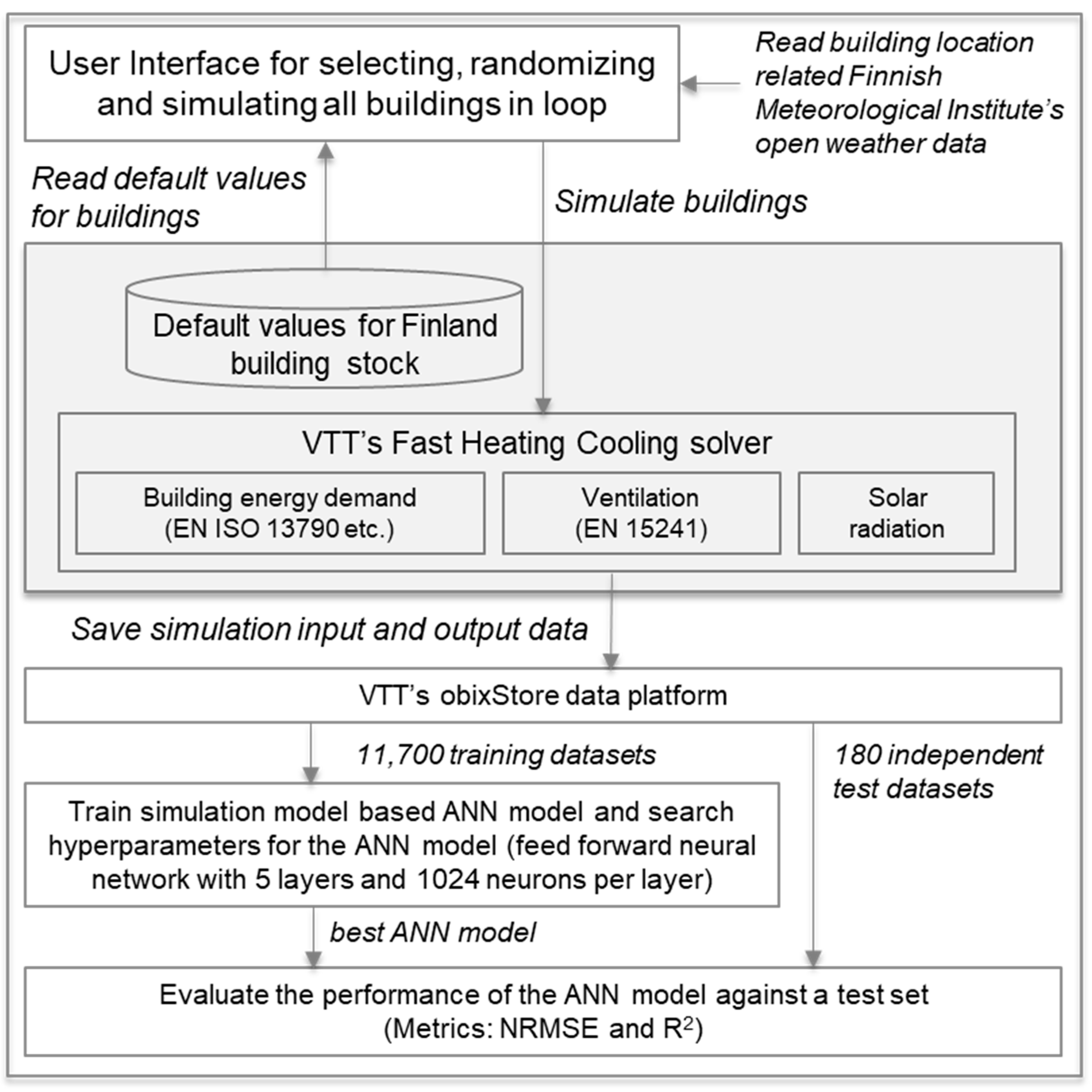
The main aim of the approach was to develop an ANN model that could be trained to represent the knowledge of an existing building simulator, the presuppositions usually made for the modelled buildings and the post processing of the simulator output. It should be clarified, that the physics-based simulator is not directly utilized in the final model, but instead used for producing training data for the ANN model. A key idea in the approach is also that the experiment is designed in a way that the ANN model has to learn to approximate the simulator in order to perform well. This includes, for example, using different buildings and geographical locations (with different weather conditions) in the training and test data sets so that the model must be able to generalize to achieve good accuracy. An overview of the methodology is illustrated in
Figure 1.
The main stages of the developing process were as follows. First, typical building parameters for the selected building types (office buildings, apartment buildings, and one family houses) were fetched from VTT’s Finland building stock default value database. The selected building model input parameters (e.g., floor areas, number of floors) were randomized to create as much variety to the training data as possible. Second, location related weather data was collected from Finnish Meteorological Institute’s (FMI) open weather data platform via RESTFul Application Programming Interface (API). Third, the randomized buildings were simulated by calling VTT’s Fast Heating Cooling solver in a loop via a RESTful API. Both simulation inputs and results were saved as a three different training sets (includes validation set for hyperparameter tuning) (11,700 simulations) and a test set (180 independent simulations). Fourth, based on the training datasets, different ANN models with different number of layers and neurons per layer were trained for each training set and the model that performed best with a validation set was selected for final evaluation. The model architecture tuning, along with other hyperparameters were searched with grid search using 10% of the training data as a validation set. It should be noted, that the main point of the paper was not to find the most optimal ANN architecture for the task, but to study and evaluate whether an ANN model learns to approximate the physics-based model. Fifth, the best ANN model was evaluated using an independent test set. These steps are described more detailed in
Section 2.2,
Section 2.3,
Section 2.4,
Section 2.5 and
Section 2.6.
2.2. Assumptions
It should be emphasized, that the methodology proposed in the paper assumes that a building simulator can accurately estimate building’s energy consumption in different conditions. It is especially important that the simulator can predict the response of a building better than a machine learning model in situations not covered by the training data. Examples of such situations include, for instance, new buildings, extreme weather conditions, and most importantly demand response (i.e., when the building’s heating is actively controller with respect to market signals). This assumption is backed up by existing work [
4,
5], but nevertheless should be carefully considered in future research.
2.3. Building Energy Simulation Models
The dynamic hourly based building energy demand simulations are performed with VTT’s Fast Heating-Cooling demand solver (Fast HC solver). It is based on EN ISO 13790:2008 (Energy performance of buildings: Calculation of energy use for space heating and cooling) and EN 15241:2007 (Ventilation for buildings: Calculation methods for energy losses due to ventilation and infiltration in buildings) standards and dynamic models for estimating solar radiation. The model considers heat losses through building envelope, ventilation, and air leakages, as well as heat gains from appliances, occupancy, and solar radiation.
The model requires a lot of detailed information of a simulated building. If all input parameters are not known, it can use representative values from VTT’s default value database [
29]. The database includes typical values for different ages of Finnish office buildings, apartment buildings and one family houses, such as building structures thermal transmittances (U-values), ventilation details and user profiles. Requirements from U-values for each construction year come from the Finnish building regulations. User profiles define running times for ventilation, and schedules for heat gains from people and appliances, these are specific for each building type.
2.4. Dataset Generation
Training and testing data are generated with the simulator described in
Section 2.2. Different building parameters are chosen randomly from a realistic range of each building type (apartment buildings, office buildings, one family houses). The data resolution for energy demand and weather measurements is 60-min.
Weather measurements from FMI of three different locations are utilized in the simulations. These locations represent various temperature zones of Finland. Helsinki is located in southern Finland by the seaside, Jyväskylä in the middle, and Sodankylä in the northern part of the country. Weather measurements are utilized instead of forecast because the goal is to study whether the physics-based simulator can be approximated by an ANN model. FMI does not also provide historical data on forecasts, just on measurements.
Three separate training sets and one test set are generated with the following configurations:
Training set 1:
- ○
Three year simulation for three locations (Helsinki, Jyväskylä, Sodankylä), 100 buildings per type per location.
- ○
Weather data includes years 2016–2018.
- ○
Contains a total of 900 buildings.
- ○
Training set is divided so that 90% is used for training and 10% for validation.
Training set 2:
- ○
One month simulation for Helsinki only, 300 buildings per building type.
- ○
Simulated months are sampled randomly from 2015 weather data.
- ○
Contains a total of 10,800 buildings.
- ○
Training set is divided so that 90% is used for training and 10% for validation.
Training set 3:
- ○
Training set 1 and 2 combined (added together as such).
Test set:
- ○
One year simulation for each of the three locations, 20 building per building type.
- ○
Year 2019 measurements are used as the weather data.
- ○
Contains a total of 180 buildings.
2.5. Feed Forward Neural Network
In order to find a good ANN model for the task, a FFNN with different number of layers, and neurons per layer were trained and evaluated with the three training (and validation) datasets. Based on the average RMSE of the validation sets, the best model was an FFNN with five layers and 1024 neurons per layer. Features were normalized with MinMaxScaler, Rectified Linear Unit (RELU) was used as the activation function for hidden layers, and Adam [
30] as the optimization method.
Table 1 summarizes the main attributes of the FFNN.
The model has identical input features to the original simulator. These 12 features include: day of the year, hour of the day, outside temperature, direct solar radiation, diffuse solar radiation, construction year, building type, floor count, cross floor area, building shape, heat recovery efficiency for ventilation, and heat capacity. Sin and cos values for both time features was used. One-hot encoding was utilized for building type (apartment, office, single family), building shape (rectangle, U-shape, L-shape, closed block, between two buildings), and heat capacity (light, medium, heavy). As typically building properties are related to the existing regulations, construction year is one-hot encoded to match known time spans of different regulations.
In order to perform well in the task, the FFNN model needs to learn both the physical building model and the associated default value database. Heating plays a much bigger role than cooling in Finland due to the relatively short cooling season. For this reason, space heating was chosen as an output for the model. Single family homes have a significantly smaller heating need, and with the current model, they had to be trained separately from the other building types.
2.6. Metrics
Normalized root-mean-square error (NRMSE) and coefficient of determination (R
2) are calculated for each building in the test set separately. In the results, the average of these values are presented based on the building type and location. Formulas used for calculating the metrics are presented in Equations (1)–(3).
where
yi is the observation,
is its mean, and
ŷi is predicted value,
ymax and
ymin are the maximum and minimum values of
y, respecctively.
It should be noted that the paper does not use the typical lead time, forecasting horizon, and update rate parameters. This is because the proposed ANN does not utilize energy consumption of the building as input, and since we utilize measured weather conditions during the evaluations (instead of weather forecasts) lead time, horizon, and update rate do not affect the accuracy. These parameters are of course important when the impact of the weather forecast accuracy to the forecast accuracy is analyzed. However, since the main point of the paper is to study whether the physics-based simulator can be approximated, it is better to use the actual measurements so that unnecessary noise is not included into the evaluation.
4. Discussion
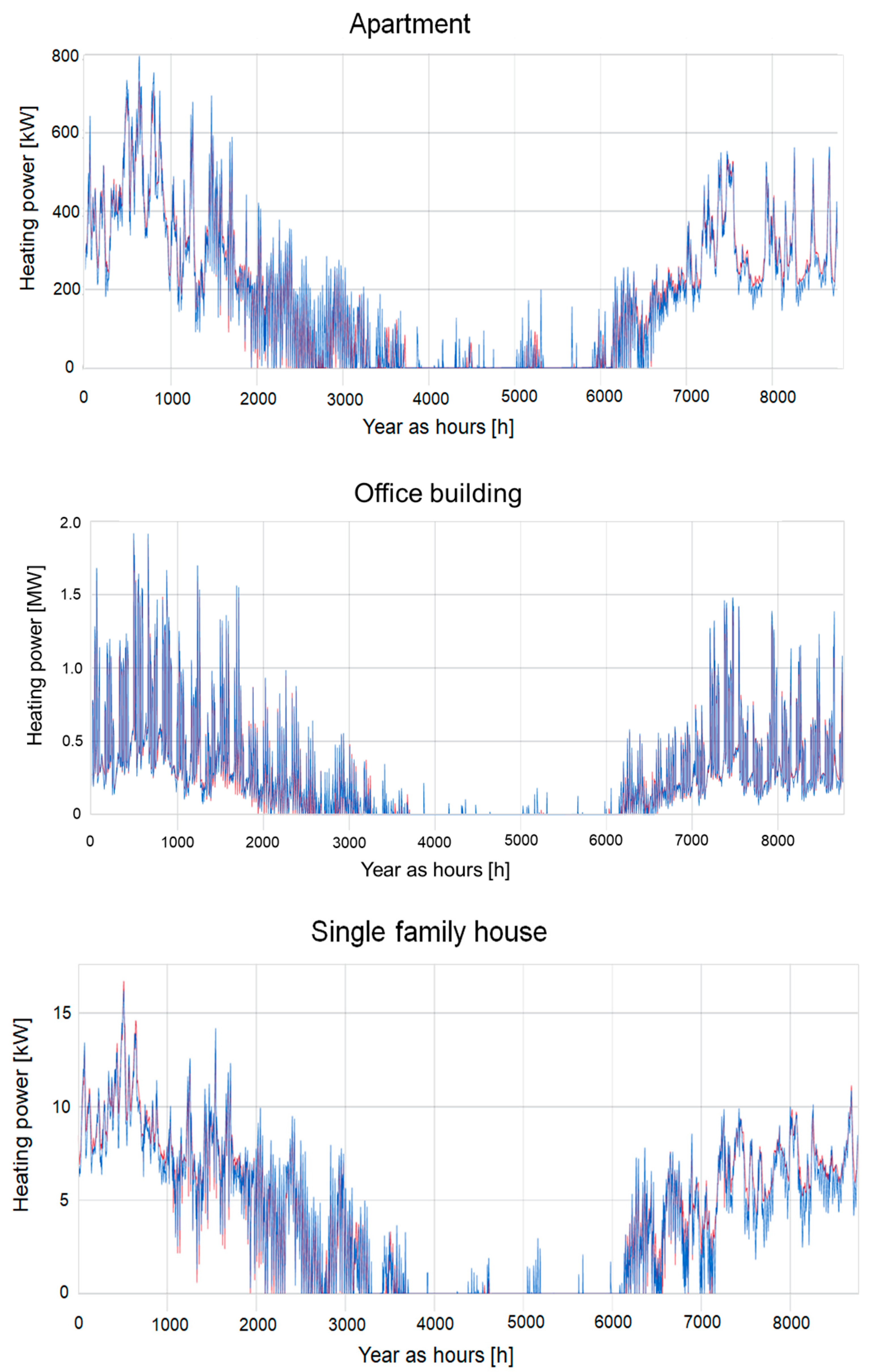
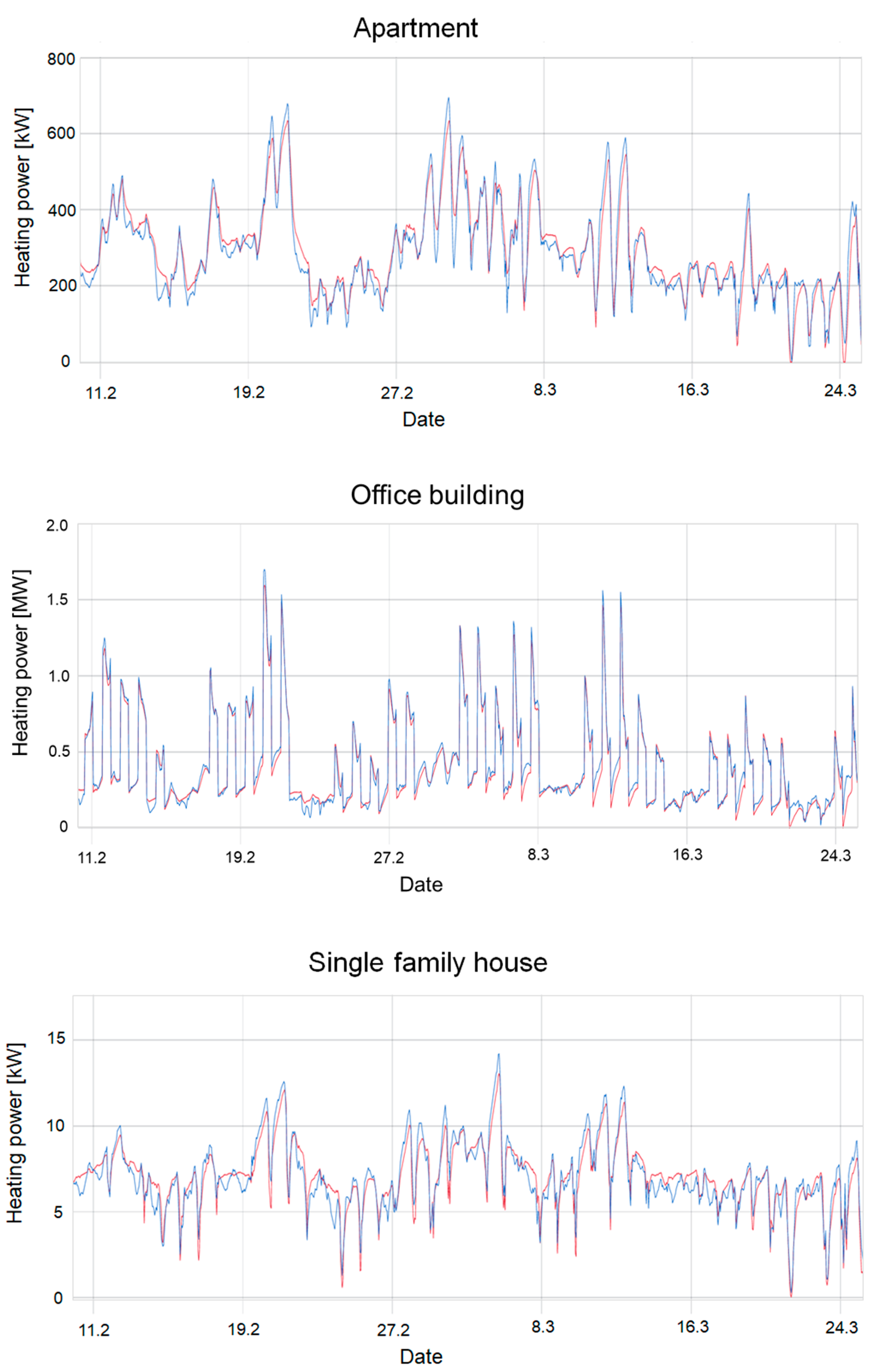
The main purpose of the study was to evaluate whether a ML model can be trained to approximate a physics-base simulator so that we can combine the best parts of both worlds. The results show that this is possible, as the proposed FFNN model achieved accurate forecast with all building types. The best accuracy with NRMSE of 0.026 was achieved with office buildings. The model NRMSE with apartment buildings and single family houses were 0.050 and 0.052, respectively.
The model performed well with all three training sets and in all geographical locations. This is especially interesting in the case of training set 2 for two reasons. First, the model had only one month of training data from each building. Second, all the buildings in training set 2 were in the Helsinki area, which is located 900 km south from Sodankylä. Helsinki and Sodankylä have naturally quite different outdoor temperature conditions during the winter. Additionally, the angle of solar radiation is different. However, solar radiation angles have typically greater impact during summer than during the heating season. Nevertheless, the results indicate that the ANN model is able to learn to approximate the physics-based simulator, as it is able to extrapolate the heat demand also to new type of weather conditions.
The main benefits of the proposed approach is that it makes it possible to replace the original simulator and the associated pre- and post-processing computations with a neural network. This makes it much easier to deploy and use the model in model-based optimization, which is important in optimal energy management and demand response. When compared to other ML-based methods proposed in the literature, the main advantages of the proposed approach are (1) that it can work without any energy measurement data (important, e.g., with new buildings), and (2) that it is more robust with respect to situations not seen in the training data due to the fact that the model has to learn to approximate the underlying physics to perform well. A good example of this robustness is that the model also achieved good performance with buildings from Sodankylä even though it was trained just with buildings from Helsinki (training set 2).
When compared to other approaches [
22,
23,
24,
25,
26,
27,
28] where a physics-based simulator is used to train a machine learning model, the main difference is that in all of the previous approaches, a separate ML model is trained for each building, whereas the approach proposed in this paper is generic for all buildings. This means that the ANN model can completely replace the physics-based simulator. The results also show that the model is able to generalize to inputs not seen in the training data, which is a positive sign that the model has learned to approximate the physics encoded into the simulator. Clear evidence of the generalization capability is that the model worked well with buildings it had not seen before. Moreover, the model was able to forecast energy consumption of colder locations (Jyväskylä and Sodankylä), although training set 2 included data only from Helsinki.
It should be emphasize that the approach proposed in the paper is not restricted to ANNs. In theory, any generic function approximator could be used instead of an ANN to approximate the physics-based simulator. An ANN model was selected for this study mainly for following reasons: (1) ANN models are highly parallel and thus provide fast inference, (2) ANN models provide gradient based optimization through back propagation, which is important when the model is used in planning and control [
17,
18,
19], and (3) ANN platforms such as TensorFlow also provide good support for model deployment in edge environments [
14,
15].
There are also limitations in the current study, and future research is needed. For instance, the current model is strictly tied to Finland due to the default value database used in the generation of simulation inputs that are typical for Finnish buildings. However, this limitation can be easily tackled by training the ANN model with a default value database that covers other types of buildings as well. Additionally, the current approach was only validated against a simulated dataset. Therefore, scientific studies are needed to validate the approach also with real building data. In this context, it would be interesting to study whether the ANN model could be fine-tuned with building specific data. This is important since there is always some differences between a real building and a simulated one. Additionally, the behavior of people can influence the heat demand and cause differences between the simulation model and the real building. In practice, this fine-tuning could be done in many ways. For instance, one approach would be to re-train the whole ANN model carefully (i.e., smaller learning rate to avoid overfitting) with building specific heat demand data. Another interesting, and more data-efficient, approach would be to freeze the original ANN model and use it to fine-tune the building-specific input parameters by backpropagating gradients through the model.
It should also be noted, that the study was implemented with weather measurement data instead of forecast. Errors in weather forecast naturally cause errors in the forecast made by the ANN model. However, the main purpose of the paper is to show that the the physics-based model can be approximated with an ANN (with loss of some accuracy) in order to gain the benefits of ANN models. In this case, it is not appropriate to include additional noise to the evaluation. Nevertheless, analyzing the impact of errors in the weather input is a relevant topic for future work.
It should be also noted that the proposed approach assumes that a high detail physics-based simulator can accurately simulate the building’s energy demand as presented in the reviews by Xiwang and Ji [
4], and by Harish and Kumar [
5]. However, detailed physics-based simulation models are not automatically more accurate in forecasting when compared to compact and dedicated forecasting and on-line optimization models. The main reasons for this are the difficulty to calibrate the model parameters, possibilities for overfitting, and structural inaccuracies in the models that cannot be compensated by parameter calibration. [
31,
32]. These are valid concerns that have to be taking into account in future research, also with the approach proposed in the paper. However, we believe that the approach can actually help to overcome these challenges. This is because the ANN model can be fine-tuned with building specific data with efficient gradient based training, which can help to overcome problems related to structural inaccuracies in the original physics-based model.
Other interesting directions for future research include (1) evaluation of the approach with different type of ANN architectures and new inputs, and (2) extending the model so that it can predict also thermal comfort inside the building as well as cooling demand of the building. In particular, having the capability to predict the indoor temperature is required if the model is used in energy efficiency and demand response and optimizations. Proper modelling of indoor temperatures might require better handling of building dynamics, e.g., by utilizing Recurrent Neural Networks (RNN) such as LSTM [
33] for weather data analytics.
5. Conclusions
This paper proposed a novel approach for combining a physics-based simulator with machine learning. The key concept in the approach is to use the physics-based simulator to generate a large dataset on different types of buildings, which is used to train a single ML model. The idea is that this would force the machine learning model to better learn to approximate the physics-based simulator and not just the particularities of a single building. This way, the approach would be more robust [
34] (i.e., also able to perform well in situations not covered in the training data) when compared to typical machine learning approaches. The advantages compared to physics-based models in turn are ease of deployment, inference speed, better support for model-predictive control, and the possibility to train and fine-tune the model with building specific data. To our knowledge, this is the first approach to learn the whole building simulator with a machine learning model. Previous work [
22,
23,
24,
25,
26,
27,
28] has focused on learning building specific models, which is a similar problem compared to learning the behavior of a single building. The advantage of the proposed approach is that it does not require a building specific model, as the model is able to generalize to new buildings. Additionally, in our setting, the model is also forced to better approximate the physics as it needs to be able to generalize to different type of buildings and weather conditions.
In order to evaluate the approach, we implemented an ANN model that takes building parameters, in addition to the typical weather and temporal data, as input. Existing physics-based model and a database of building attributes were used for generating the training, validation, and test datasets. The datasets included equal distribution of office buildings, apartment buildings, and single family houses. The NRMSE were on average 0.026, 0.050, 0.052 for office buildings, apartment buildings, and single family houses, respectively. The results show that the ANN model is able to accurately forecast the heat demand of different type of buildings without any energy consumption data from a given building. In order to do this the machine learning model had to learn to approximate the physics-based simulator. A good example of the extrapolation capabilities of the model was that it was able to accurately forecast the energy consumption of buildings located in Sodankylä, even though only buildings in Helsinki where present in the training set. Sodankylä is located approximately 900 km north from Helsinki, and has much colder temperatures during the winter.
Although the results are promising, more research is still needed. For instance, an interesting future research direction is to investigate approaches for fine-tuning the model with building specific data. In this context, it will be interesting to compare the approach to state-of-the-art ML models and compare the accuracy and data efficiency. Moreover, extending the approach for modelling indoor temperature and cooling demand are needed. These extensions will likely require experimentation with different type of ANN model architectures such as LSTMs to better handle the building dynamics.


