Article

A Hybrid Method for the Run-Of-The-River Hydroelectric Power Plant Energy Forecast: HYPE Hydrological Model and Neural Network

1
Dipartimento di Energia, Politecnico di Milano, via La Masa 34, 20156 Milano, Italy
2
Milano Multiphysics S.r.l.s, Polihub, via Durando 39, 20158 Milano, Italy
*
Author to whom correspondence should be addressed.
These authors contributed equally to this work.
Forecasting 2020, 2(4), 410-428; https://doi.org/10.3390/forecast2040022
Submission received: 15 September 2020 / Revised: 2 October 2020 / Accepted: 5 October 2020 / Published: 15 October 2020
(This article belongs to the Collection Energy Forecasting)

Abstract

:
The increasing penetration of non-programmable renewable energy sources (RES) is enforcing the need for accurate power production forecasts. In the category of hydroelectric plants, Run of the River (RoR) plants belong to the class of non-programmable RES. Data-driven models are nowadays the most widely adopted methodologies in hydropower forecast. Among all, the Artificial Neural Network (ANN) proved to be highly successful in production forecast. Widely adopted and equally important for hydropower generation forecast is the HYdrological Predictions for the Environment (HYPE), a semi-distributed hydrological Rainfall–Runoff model. A novel hybrid method, providing HYPE sub-basins flow computation as input to an ANN, is here introduced and tested both with and without the adoption of a decomposition approach. In the former case, two ANNs are trained to forecast the trend and the residual of the production, respectively, to be then summed up to the previously extracted seasonality component and get the power forecast. These results have been compared to those obtained from the adoption of a ANN with rainfalls in input, again with and without decomposition approach. The methods have been assessed by forecasting the Run-of-the-River hydroelectric power plant energy for the year 2017. Besides, the forecasts of 15 power plants output have been fairly compared in order to identify the most accurate forecasting technique. The here proposed hybrid method (HYPE and ANN) has shown to be the most accurate in all the considered study cases.

1. Introduction

In a context of increasing penetration of renewable energy plants, accurate and reliable energy forecasts of wind/solar/hydro power and electric loads are required by diverse types of end users (e.g., utilities, TSOs, energy traders, producers), to be implemented for different time horizons, depending on the specific application, to significantly improve their profitability [1]. Hydropower is the largest source of renewable electricity in the world, generating 16.4% of the world’s electricity production and providing 71% of renewable energy delivered to the grid, for a total capacity of 1200 GW installed power in 2016 [2].
Hydroelectric plants can be divided in three main categories: Storage Hydro Plants (SHPs), Pumped Storage Plants (PSPs), and Run-of-the-River Plants (RoR). SHPs store water in a reservoir, typically by means of a dam, and water can be released when is needed to generate power. PSPs exploit a lower and an upper reservoir to pump or release water when it is more economically convenient; it is designed to balance peak loads and it is a net consumer of energy [3]. RoR plants have small storage capacity, typically few hours; these plants lie along a river course and hence are those more influenced by climate variability and river flow changes. Forecasting activity in power generation aims to predict non-programmable energy sources; non-programmable energy production plants comprises those power plants whose generation is affected by the variability of natural resources throughout hours of the day and seasons: therefore, hydroelectric production forecast concerns RoR hydropower and not storage or pumped-storage plants.
Hydrological models are widely adopted for hydropower generation forecast as they provide effective methods to describe complex water cycle processes [4]. Among them, the HYPE model is one of the many hydrological models today adopted. Other existing models are the HBV [5] or SWAT [6], and many others [7,8]. The Hydrologiska Byrans Vattenbalansavdelning (HBV) model is a conceptual model of catchment hydrology which simulates discharge using rainfall, temperature, and estimates of potential evaporation. The HBV model [5] has been applied in numerous studies, e.g., to compute hydrological forecasts, for the computation of design floods, or for climate change studies. The Soil and Water Assessment Tool (SWAT) is a conceptual, continuous time model that was developed in the early 1990s to assist water resource managers in assessing the impact of management and climate on water supplies and non-point source pollution in watersheds and large river basins. The model SWAT is meanwhile used in many countries all over the world. The HYPE model, that will be described in deep at the beginning of Section 2.3, has been selected among the pool of existing hydrological model due to its suitability for continental or multi-basins analysis [9].
Data-driven models are nowadays the most widely adopted models in hydropower forecast [10]. Stochastic models such as ARIMA [11,12] or Persistence [13] are extensively used; in particular, the persistence model can be applied to RoR plants, which typically have high autocorrelation with the preceding day. Machine learning (ML) models are increasingly applied to hydrological forecast and have addressed and solved many issues in hydrological modeling [14]. In particular, Artificial Neural Network (ANN) is widely adopted [15,16,17] due to its strong adaptability and learning ability [18], resulting as one of the most successful ML methods. In [19], it is shown the superiority of ANN in respect of other ML techniques in hydroelectric forecasting, while in [19] it is compared the deployment of ANNs and persistence model, proving again a higher accuracy when neural networks are employed. ANN basically consists of a number of neurons grouped in different layers, which receive the input from all the neurons in the preceding layer [15]. An artificial neuron is formed by n channels in input, each one having a weight that represents the connection force through the corresponding channel [20]. The output layer represents the variable to predict; during the training process a certain number of input and output samples are evaluated from the network, which modifies weights in order to minimize the overall error committed. Once the network is trained it is possible to provide the input data to the network, which will return the forecast of the output variable.
Further research for forecast improvement is conducted in the field of hybrid (blended) methods. These models have been introduced to solve the weaknesses of individual methods and to enhance their strengths and accuracy [21]. Hybrid models blend two or more techniques in various steps in order to deliver a single forecast. Generally hybrid methods perform better than single techniques [22]. Diverse ensemble methods have been developed in last decades for hydropower production. In [23], for example, a hybrid of ANN technique with Bat Algorithm is investigated, while in [24] a least squares support vector regression ensemble learning approach is proposed. In [25], instead, proposes a data-driven blended model, named CEREF, based on the combination of empirical mode decomposition, radial basis function neural networks, and external forces variable, for hydro stream-flow forecast.
Hydropower plants, and in particular Run of the River plants, show a seasonality pattern in their production time series [26]. Therefore, a decomposition approach is often investigated to overcome the difficulties in forecasting hydropower production, applying a so called “decomposition and ensemble” approach [24], separating the different components of the time series to forecast them individually and to subsequently recompose the series to get the final prediction. In [27], it is shown how an ensemble empirical mode decomposition, hybridized with an ARIMA approach, allows to improve the ARIMA forecast performance. The authors of [28] analyze the effect of detrending and deseasonalization on neural network performance, highlighting how ANN finds it difficult to manage different components of the data simultaneously and the beneficial effect of time series preprocessing. In [29], alternative seasonality extraction approaches to the classical moving average decomposition to be coupled with simple forecasting techniques are proposed. Further analysis on decomposition approaches are proposed in [24,30].
In the present paper, a new hybrid method for hydropower production forecast is introduced. The proposed approach leverages on the ensemble of a HYPE model, that relates weather forecasts to rivers flow, with an ANN. Additionally, the model is validated considering a decomposition of the time series in three main components: trend, seasonality, and residual. As a benchmark, it is considered the ANN, with the whole time series in input. Intermediate combination are also evaluated (ANN with time series decomposition and hybrid method) to highlight the contributions of the two proposed approaches.
The paper is outlined as follows. Section 2 presents the available dataset and the method developed to analyze it and improve the power generation forecast. Section 3 reports the results obtained from the implementation of the proposed method, in comparison to a traditional ANN forecast, and discusses the results while Section 4 sums up the work performed.

2. Materials and Methods

The here presented work aims at evaluating the forecasting performance of the proposed hybrid method, composed by a HYPE hydrological model and a ANN method. The model is applied on the power production time series decomposed in trend, residual and seasonality. This approach (Hybrid plus Decomposition) is then compared to three benchmark models: Hybrid, ANN, and ANN plus decomposition.
This section is structured as follows. At first, the available dataset for the proposed method validation is presented and described. In the second part, the error metrics adopted to evaluate the performance of the investigated methods are discussed. Finally, in the last subsection the novel hybrid method for RoR hydroelectric production forecast is detailed.

2.1. Available Dataset

The dataset adopted to validate the proposed method is referred to Slovenia and consists of two parts: flow data and measured electric hydropower production in the period from January 2010 to December 2017.
Slovenia is modeled dividing it into 86 different sub-basins. The conditions and geographic features of each sub-basin are exploited by the HYPE model to return the inflow of the drainage basin (an area of land where precipitation collects and drains off into a common outlet, such as river, bay, or other body of water). In our specific case, just precipitations data are provided to the HYPE model, since rain is the main driver in hydropower generation. It has been collected rainfall daily data, measured in [mm], of three Slovenian meteorological stations. Climate data are taken from the “Copernicus Era5” meteorological database and are of public domain. For each sub-basin, geographical data are provided and a basin map based on sequentiality of sub-basins has been drawn: in particular three groups have been identified, and these groups of points represents the river-basin of the three main Slovenian watercourses: River 1, River 2, and River 3, represented in Figure 1.
The second part of the dataset is made by the hydroelectric energy produced [MWh] from 2010 to 2017 and Hydro-States, that informs about the status of each plant (working or not). The final purpose of the analysis is to predict the electric production of hydroelectric power plants, and specifically of big power plants (rated power P e l > 20 MW). The dataset is cleaned by discarding those plants characterized by zero-production for a period greater than the 10 % of the total number of samples: three plants have been excluded, for a total of 15 RoR remaining plants, distributed on three rivers: 3 plants on River 1, 5 on River 2, and 7 on River 3. The preprocessing performed on the dataset aimed at testing the proposed method on a significant set of data, with few missing values, to evaluate its performance. The null power production observed in a plant could be due to human regulation rather than a lack of minimal flow in the river, uncoupling in this way the production from the Rainfall/CSB flow forecast. These cases are unpredictable by the algorithm, since they do not derive from a physical process and we have therefore decided to exclude them.
Data are converted on daily basis to have the same time-step of flow data. To validate the proposed method, all the available plants have been studied.

2.2. Performance Measurement

In the present work a series of indicator has been defined to evaluate the goodness of the prediction, in order to address different issues. Among the existing performance metrics, we selected the normalized Mean Absolute Error (1) (nMAE [31]) to evaluate the overall performance:
n M A E = 1 N k = 1 N W k f o r e W k o b s C
where N is the total number of data sampl;, C is the maximum power measured over the period under analysis; and W k f o r e and W k o b s e are, respectively, the forecast power and the measured (observed) power at each time point. In addition, two metrics have been introduced. The Nash–Sutcliffe Efficiency Index E f (2) is commonly used to assess the performance of rainfall runoff models [32]; it varies in the range ( , 1 ] , where the unity is obtained in case of perfect forecast. The latter metric considered is the MASE (Mean Absolute Scaled error) (3), which is little influenced by the outliers [22]:
E f = 1 k = 1 N ( W k f o r e W k o b s ) 2 k = 1 N ( W k o b s W ¯ o b s ) 2
M A S E = 1 N k = 1 N ( W k f o r e W k o b s ) 1 N 1 k = 2 N ( W k o b s W k 1 o b s )

2.3. HYPE model and hybrid forecast method

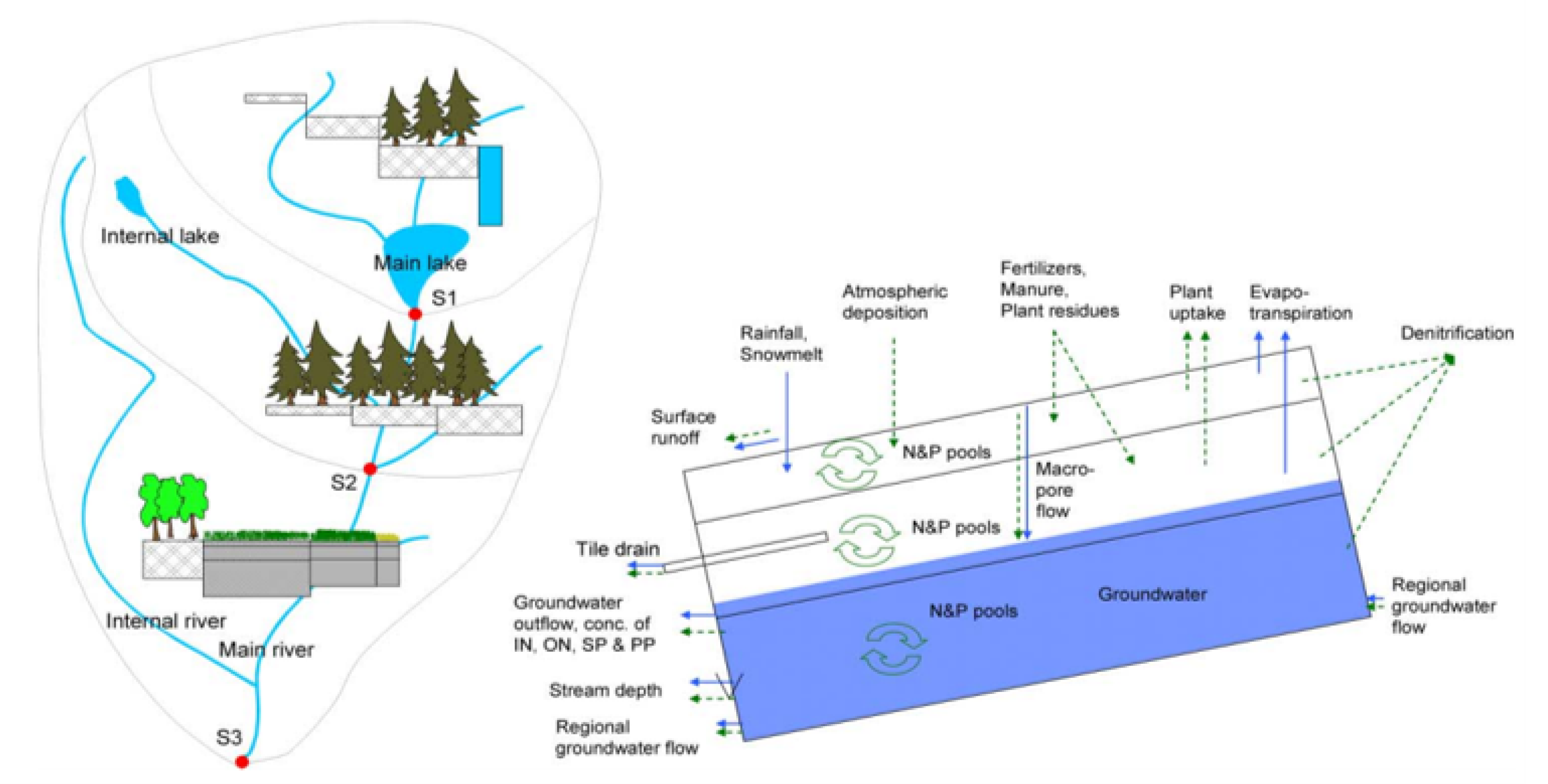
The Hydrological Predictions for the Environment (HYPE) model, is a dynamic, semi-distributed, and process-based model leveraging on well-known hydrological and nutrient transport concepts. It can be used for both small and large scale assessments of water resources and water quality developed at the Swedish Meteorological and Hydrological Institute during the period 2005–2007 [33]. In the HYPE model applications, which simulates water flows [34,35,36], the model domain may be divided into sub-basins, that can either be independent or connected by rivers and a regional groundwater flow, as exemplified in Figure 2.
The model receives as input climate variables, rainfall, and ambient temperature among the most important, and returns the sub-basins’ water flow with a daily time step as output. An overview of the typical input data for the HYPE model is provided in [33], while in [37] a review of those input parameters that majorly influence performances of the model is presented. The HYPE model is particularly appropriate to simulate ungauged catchments, it is made on simple conceptual and empirical equations, and represents one of the best options for large-scale continental or multi-basins simulations [9]. Therefore, HYPE model was selected to compose the here presented hybrid method.
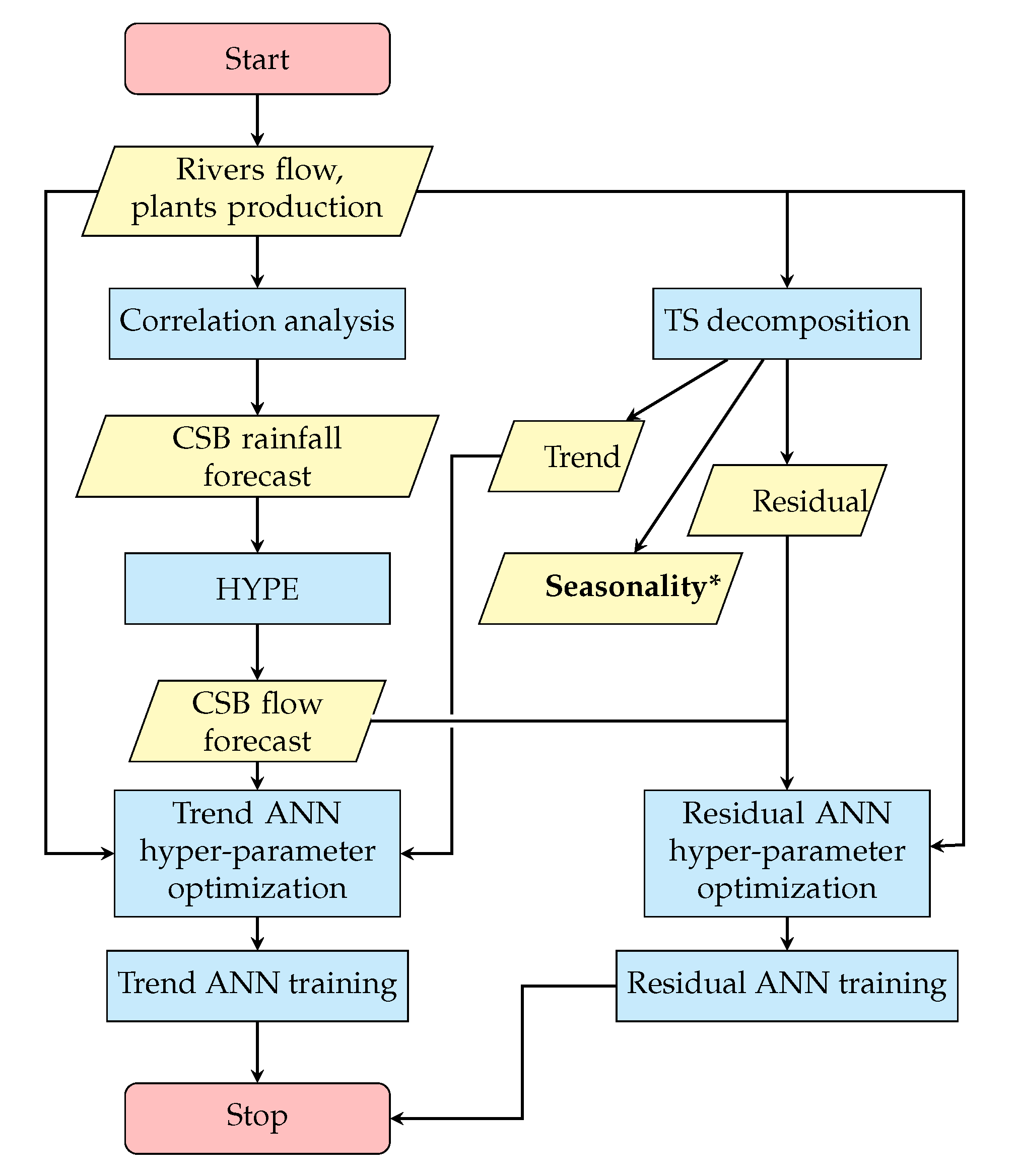
In Figure 3, the adopted method and the process required to train the hybrid network is displayed. The yellow parallelogram highlights the input/output datasets obtained, while the light blue rectangles highlights the processes performed. At first, it is conducted an analysis to identify the most suitable inputs to be fed into the neural network. A correlation analysis is therefore performed, to select the highly Correlated Sub-Basins (CSB) to the considered plant. The rainfall forecast associated to the identified sub-basins is then fed into the HYPE model, that provides the CSB outflow forecast. In parallel to this analysis, a decomposition of the production time series of the considered plant is performed, identifying the Trend, Seasonality*, and Residual components. The second term will be then used in the forecast process (Figure 4). Trend and residual components, together with the considered plant past production and the CSB flow forecast, are exploited to perform at first the hyperparameter optimization for the Trend and Residual ANN sizing, respectively, and then for the network training itself.
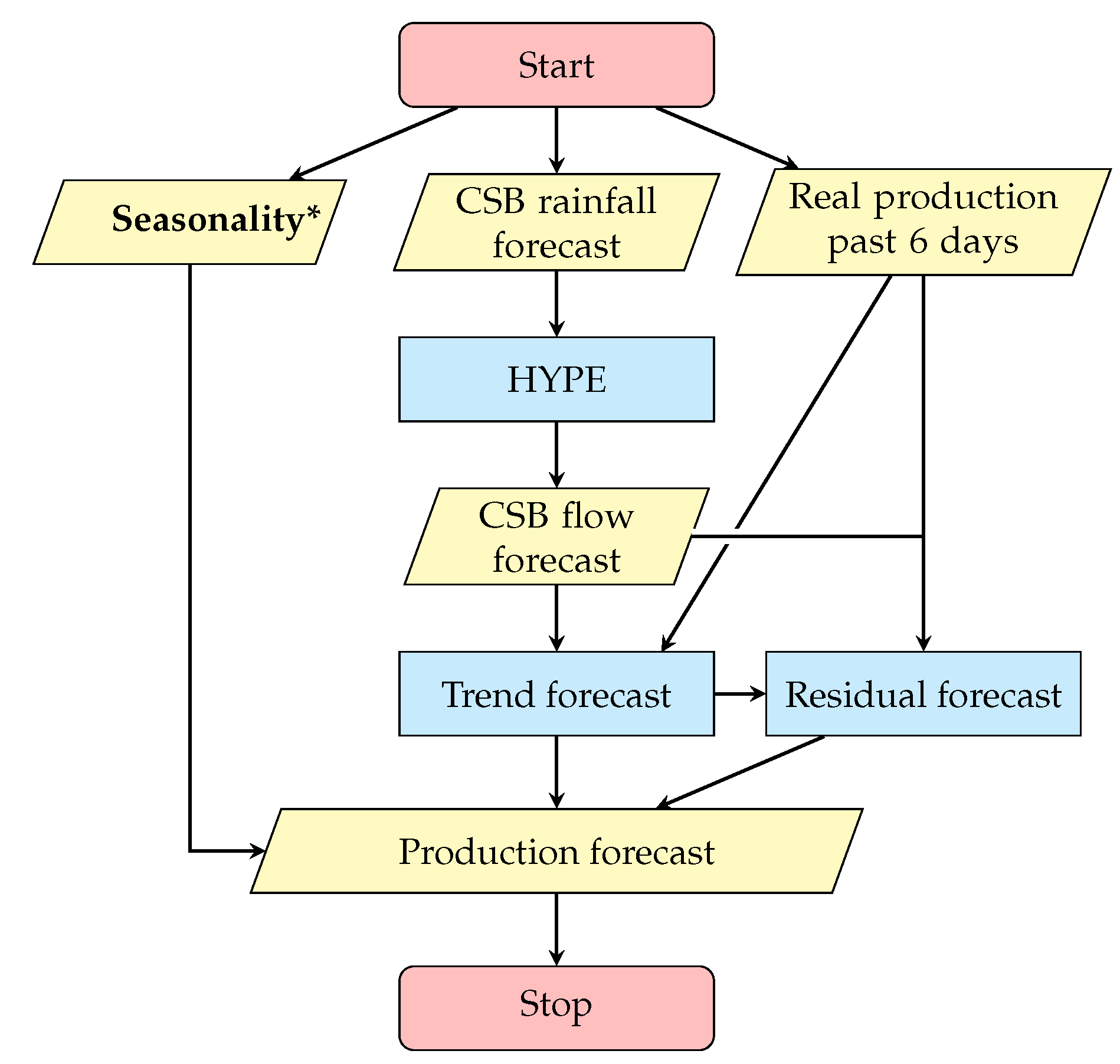
Once the proper network structure is identified, the forecast will be performed, according to the scheme reported in Figure 4. The CSB flow forecast and the real production of the past six days are exploited to get the trend forecast. This forecast is then fed, together with the previous inputs, into the residual ANN, to get the residual forecast. The obtained production components are then summed up to the seasonality profile to get the production forecast. The obtained results are compared to those coming from the adoption of the ANN (without decomposition), which receives as input the same elements of the HYPE model, i.e., the input weather data from national databases. Additional configurations are considered: Hybrid and ANN with decomposition, to highlight the contributions of decomposition and hybrid network, respectively.
Analyzing the process in detail, at first an analysis on correlation factors is conducted, in order to establish the input–output connection and to identify the proper input layer to feed the ANN. The aim is to understand how the energy production is linked with the discharge flow rate of all basins, in order to find groups of sub-basins which are more relevant for the production; when these groups of basins are estimated, their data values will be exploited to feed a neural network, by exploiting just the highly correlated sub-basins.
ρ x y = i = 1 n ( x i x ¯ ) ( y i y ¯ ) i = 1 n ( x i x ¯ ) 2 i = 1 n ( y i y ¯ ) 2
The correlation coefficient (4), ρ , measures the strength of the linear relationship between two variables x and y. When the value of ρ is near zero, it indicates the absence of a linear relationship. Generally, we consider the correlation between two variables to be strong when 0.8 ρ 1 , weak when 0 ρ 0.5 , and moderate otherwise [38]. The analysis allowed to associate at each power plant a list of sub-basins that majorly contribute, from the correlation point of view, to the hydroelectric generation and to identify the most correlated plants. In particular, it emerges that plants on River 3 have a high correlation with very few sub-basins, which largely correspond to those basins contributing to River 3 from sequentiality point of view. Instead, plants on River 1 and River 2 are both highly correlated to many more sub-basins, and especially they have many correlated sub-basins in common, which do not correspond to those identified from the sequentiality logic.
A decomposition procedure is then introduced to separate the different contributions of the series. Decomposition is used in time series analysis to describe the trend and seasonal factors in a time series. One of the main objectives for a decomposition is to estimate seasonal effects that can be used to create and present seasonally adjusted values [39]. One of the strengths of the ANNs is their ability to infer nonlinear relationships between the input and the output [40], as ANN leverage on a nonlinear activation function, therefore a simple correlation analysis and moving average decomposition approach [41] has been adopted, reported in (5).
O b s e r v e d = T r e n d + S e a s o n a l i t y + R e s i d u a l s
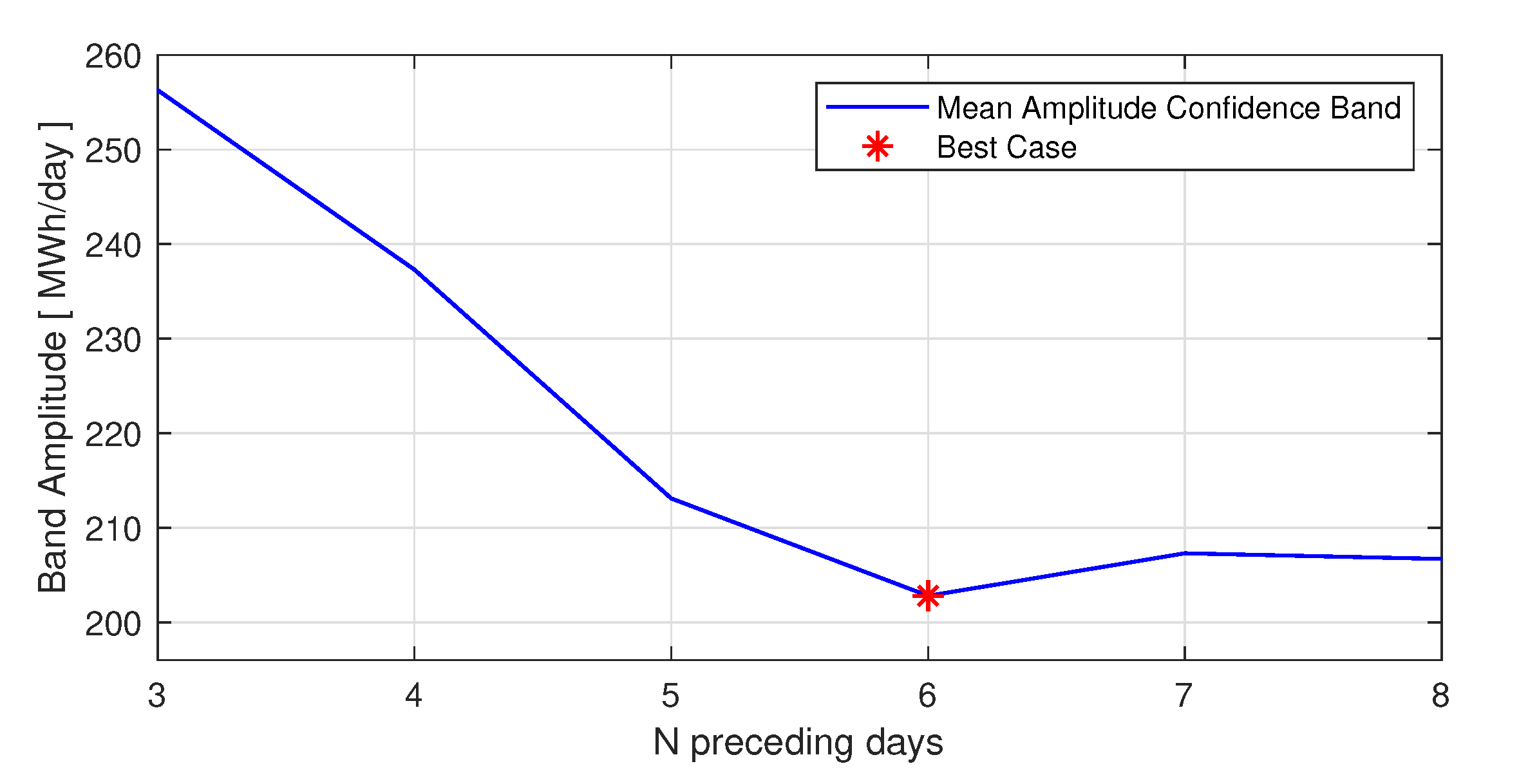
The trend is detected by applying an asymmetrical moving average, with a moving window referred to the past “N” days, thus a methodology that allows to find the best number of past days to apply the moving average is investigated. A statistical approach exploiting confidence interval is adopted. In particular, an adaptive confidence band is implemented, where the band is time-variant and it is computed on the basis of the “N” past days. The objective is to find what is the number such that the 90% of the real data are contained in the confidence band and which of these numbers guarantee the smaller band. At first, it is extracted the trend, applying the mean of the N past samples, for each day D of the dataset, where Observed is the real production dataset and D is the number of samples (from 1 to 366) (6). Subsequently it is computed the error, defined as the difference between the real production and the extracted trend, evaluated from the preceding N days to the day D (7). Finally, on the basis of the standard deviation σ of the error, proportional to the error committed in the past N days, it is found the confidence band amplitude. C is a multiplicative factor to guarantee the inclusion of 90% of real data in the confidence band (8). For the sake of simplicity the value of “N” preceding days varies from 3 to 8.
T r e n d D , N = k = D N + 1 D O b s e r v e d k N
E r r o r D , N = [ O b s e r v e d D N + 1 T r e n d D N + 1 , , , O b s e r v e d D T r e n d D ]
B a n d D = C · σ D = E r r o r D , N E r r o r ¯ D , N N
The number of samples to be included in the moving average has been set equal to 6 days, according to the sensitivity analysis led (Figure 5).
The difference between the starting ( O b s e r v e d i ) time series and the new trend function ( T r e n d i ) is called Ripple (9) and it contains the sum of the seasonal and residuals components.
R i p p l e i = O b s e r v e d i T r e n d i = S e a s o n a l i t y i + R e s i d u a l i
The ripple dataset is then divided in many subsets as the amplitude of the window moving average, 7 in our case (6 previous days plus the day to be forecast), forming 7 datasets containing the ripple component of every day of the week along the whole dataset, as exemplified in (10).
R i p p l e M o n d a y = [ R i p p l e i , R i p p l e i + W , , R i p p l e i + D · W ]
To obtain the seasonal component, the arithmetic mean of each R i p p l e subset is performed (11). The seasonality dataset is made by 7 terms repeated periodically, being the average value of the deviation between the real production and the trend.
S e a s M o n d a y = 1 D k = 1 D R i p p l e M o n d a y
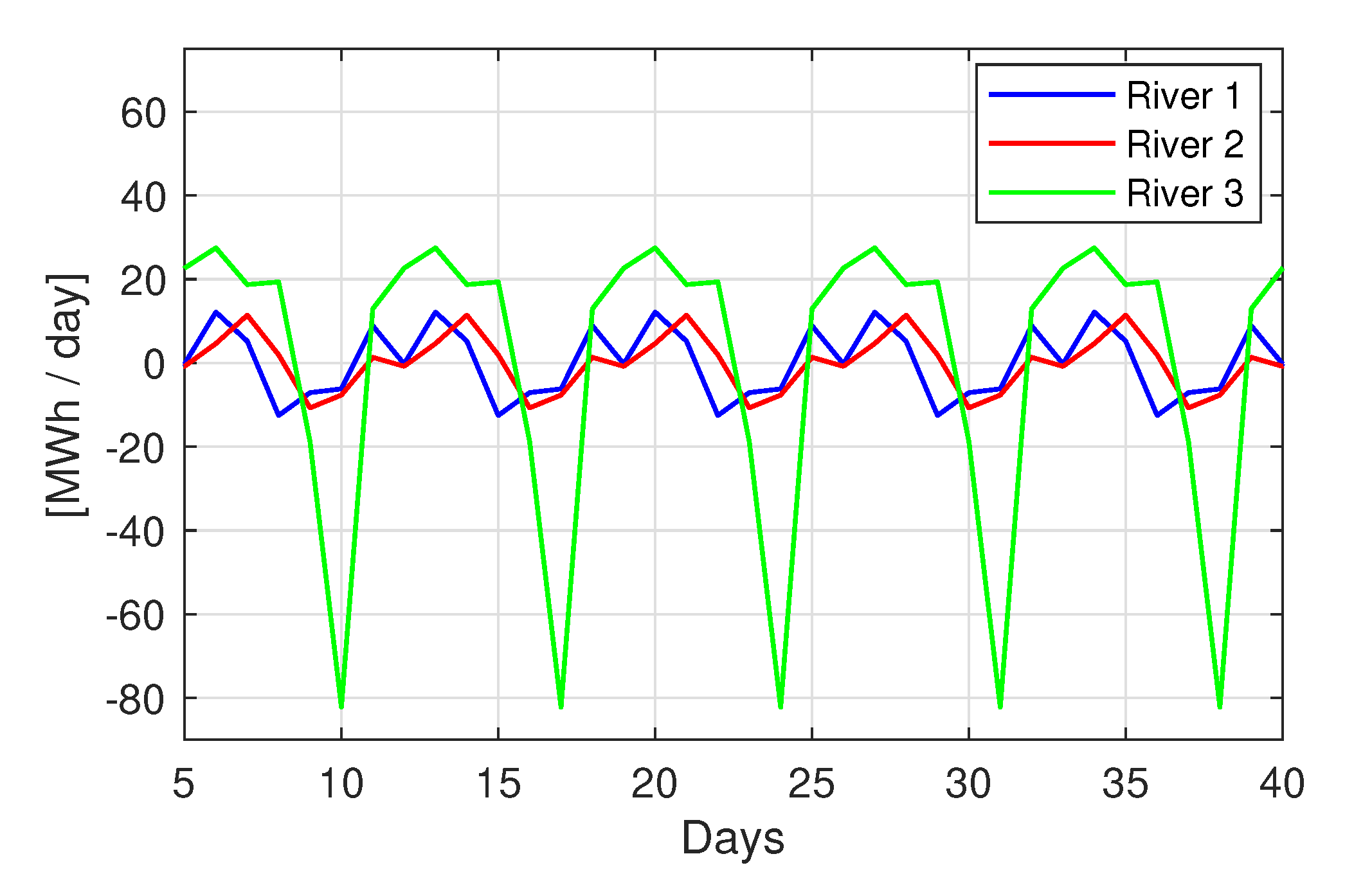
It is important to underline that “seasonal” refers to a “statistical seasonality”. In Figure 6, the seasonal component of three power plants on the three different rivers is represented. The plant on river 3 is characterized by an amplitude in the seasonality profile more stressed than in the other two, therefore it is reasonable to expect that this plant will benefit more than the other two from a decomposition approach.
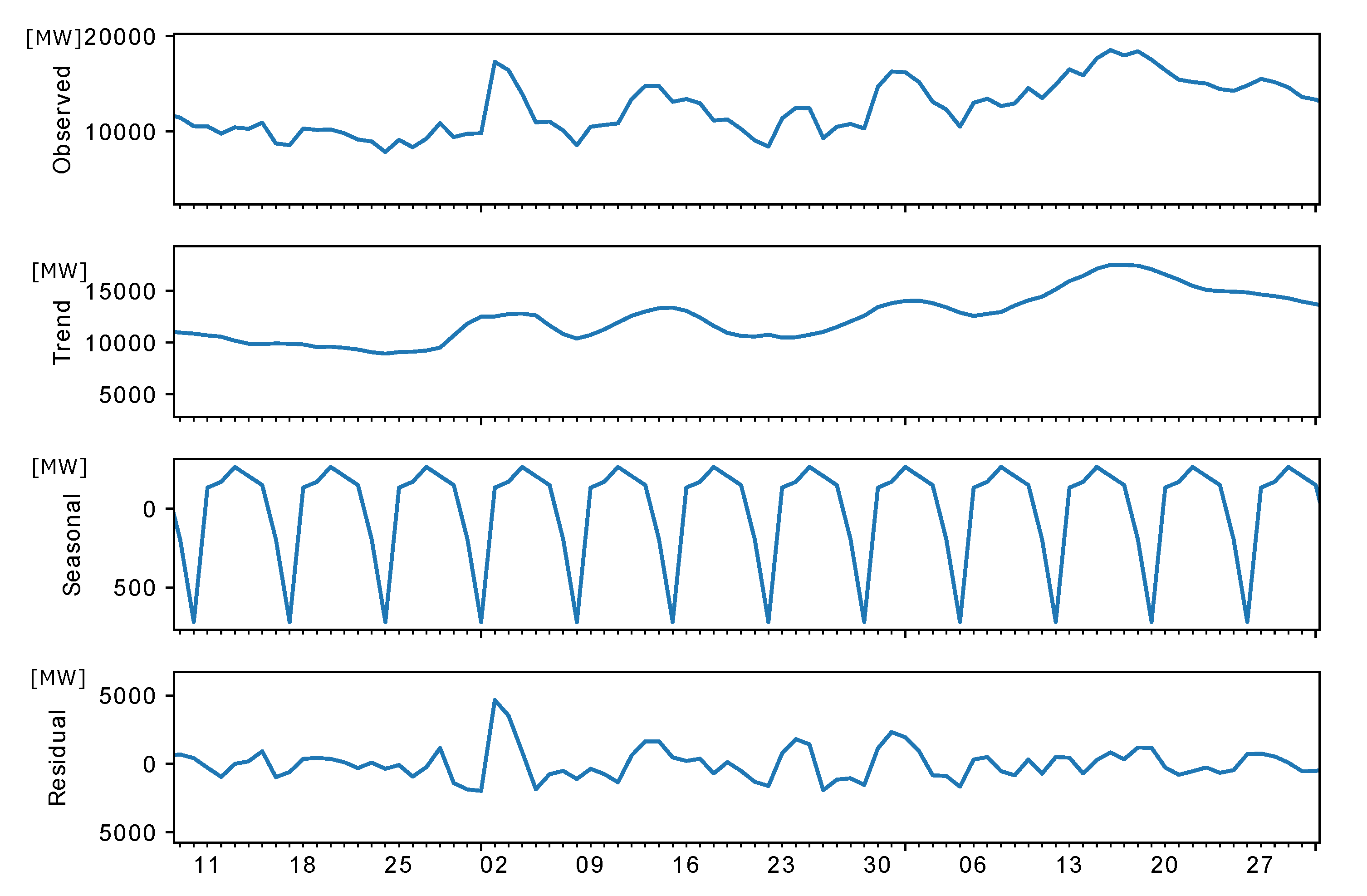
The remaining component is the residual which contains information about the “irregularities” found in the time-series decomposition. Figure 7 shows graphically the extraction of the three components from the observed production of a selected plant. It is evident how the trend is characterized by a smoother profile, with less noise, while the residual absorbs all the “irregularities”. The seasonal component is used to analyze and understand the dynamics of the electric production and the behavior of the river on which the hydroplant lies. To apply the above described decomposition it is exploited the Python function seasonal-decompose, imported from the “statsmodel” library (which is taken from the “stats” package of R language).
On top of the obtained decomposition, the training of the ANN can be set. The novel hybrid approach proposed is characterized by two ANNs having as output layer the trend in one case and the residuals in the other, which will be then summed up to the seasonality component previously extracted to recompose the function, according to (5).
A preliminary analysis is conducted in order to assess the order of magnitude of the main parameters of the network: the size of the training set, the number of hidden layers, and the number of neurons in each hidden layer [42,43]. A hyperparameter optimization is performed varying the training set size and the number of neurons, selecting the combination of parameters that minimizes MAE. The number of neurons is assumed varying in the range [2,40] with step 2.
The three models selected for the comparison undertook themselves a hyper-parameter optimization to properly design their structure.

3. Results and Discussion

The analysis is carried out on the selected hydro plants and tested in the period from 1 January 2017 to 31 December 2017. The training of the networks is performed on the days of the year 2016. As input to the networks is provided the observed power production of the six preceding days to the day to forecast (moving window approach).
From the analysis conducted on correlation factors, it has been decided to provide as input to the neural network just the sub-basins highly correlated with the chosen plant ( ρ > 0.5), in order to delete those basins scarcely correlated to the plant production. The hyperparameter optimization conducted allows to identify the optimal neural network configuration in order to carry out the forecast. In Table 1, the results of the analysis and the parameters settings adopted are summarized: the number of inputs is function of the number of CSB identified.
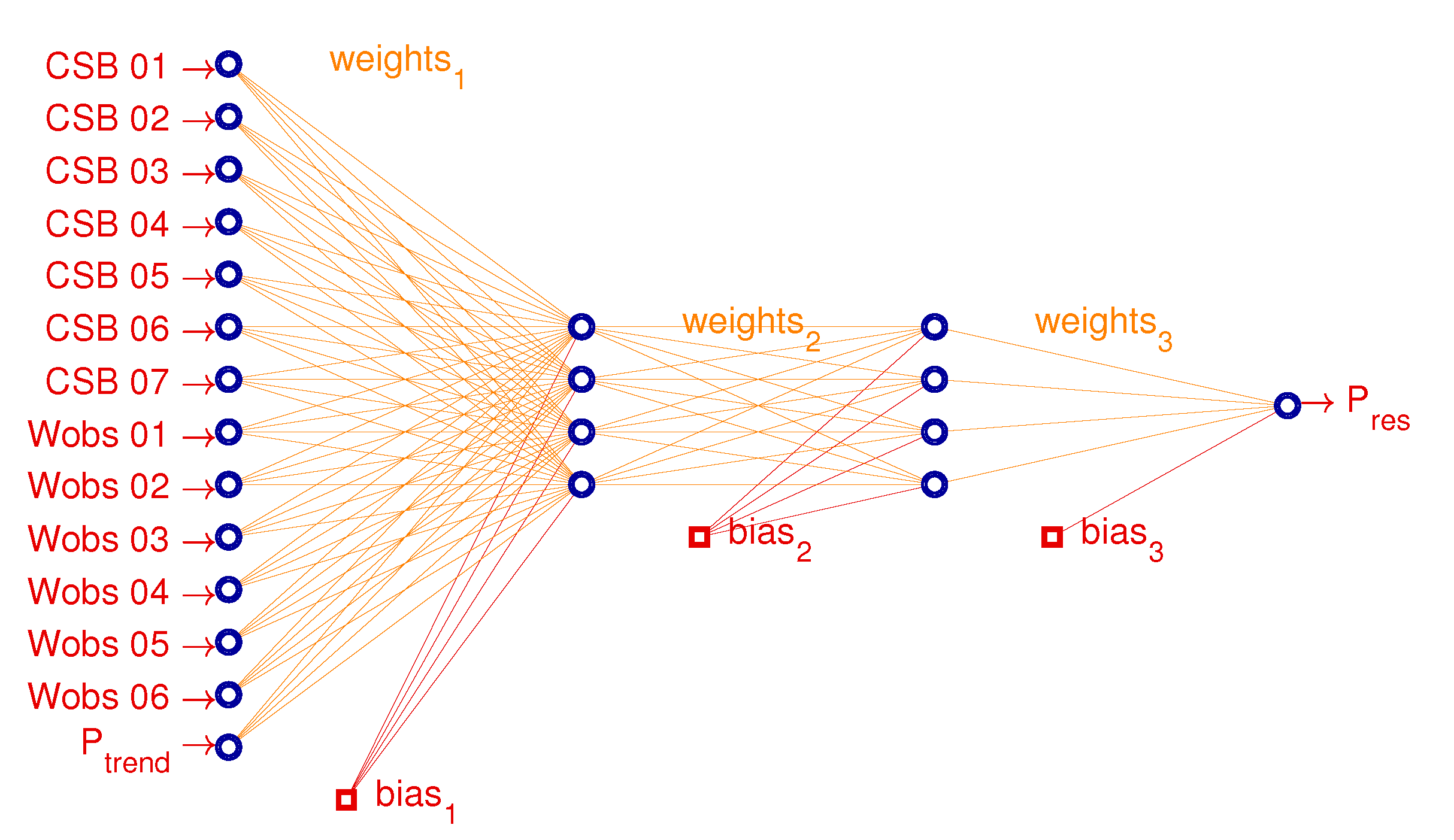
Before starting the training process, the network automatically normalizes the inputs, to speed up the simulation and reduce the computational burden. The activation function implemented in the ANN is the tansigmoid one. It can be noticed that the trend forecast requires a very low number of neurons and a short training set, just 50 days, due to its smoother profile. Residual forecast leverages on a huger TSS, of 100 days, and on a two layers network, each of them made by four neurons. In Figure 8 is represented the Residual ANN structure of the plant 2, river 3: it takes in input the CSB flow (CSB xy), the production of the previous six days (W o b s xy) and the trend forecast (P t r e n d ).
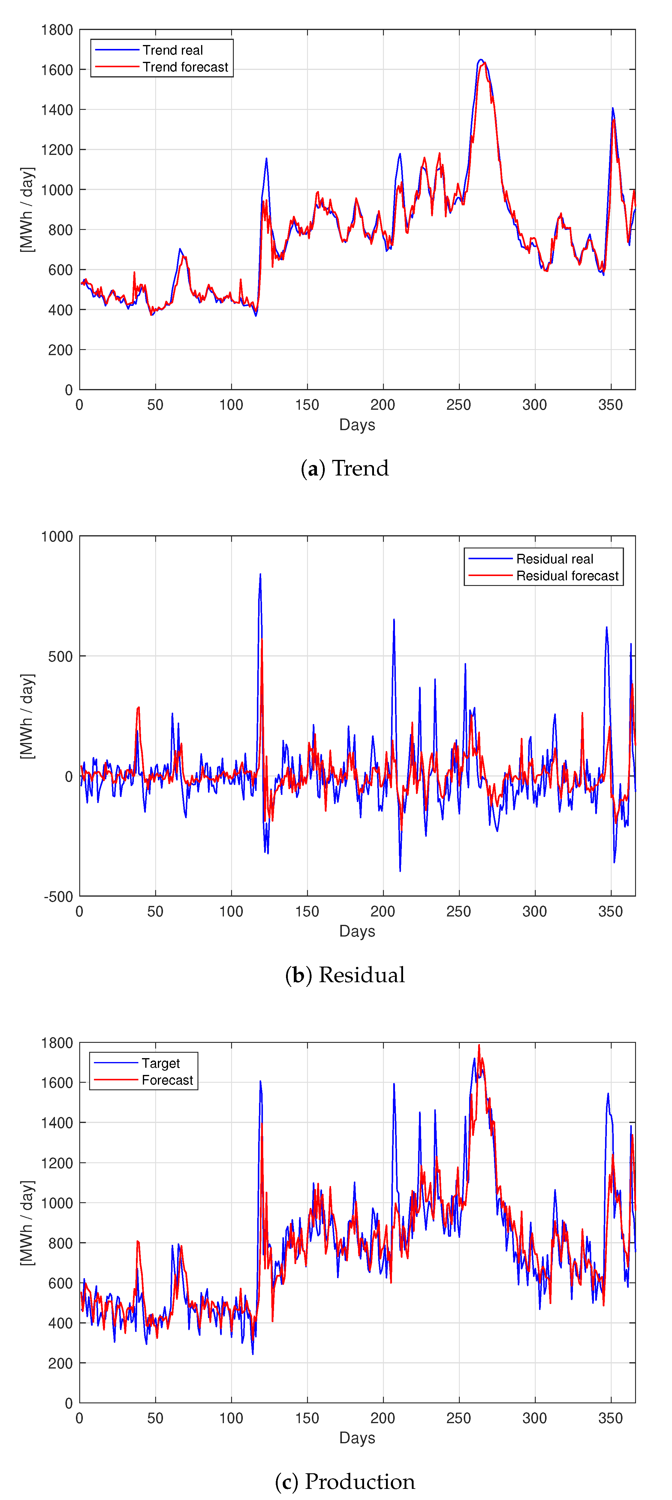
To get the overall foreseen production, the trend and residual forecasts are summed to the seasonality extracted in the decomposition procedure. In Figure 9 are reported the three phases of the decomposition approach: trend (Figure 9a) and residual forecast (Figure 9b) in order to obtain, once these components are summed to the extracted seasonality, the overall production forecast (Figure 9c). As it is possible to observe, the network is able to predict quite accurately the trend behavior, while the residual forecast is less precise and has the aim to detect the sudden increase or decrease of energy production, for instance, around day 120 (positive and negative peaks), or between days 200 and 250 (negative peaks). In the recomposed forecast (Figure 9c) the majority of the peaks, the most difficult to be predicted, are now well interpolated; negative peaks until day 120 are well represented thanks to the seasonality contribution: these negative peaks occur during Sundays. RoR plants can have a small storage capacity (pondage), which can imply the possibility of a limited amount of power regulation, that allows the producer to generate more electric power when electric prices are higher (mid-week), and generate less when prices are lower (weekend). The objective of the seasonal component is to detect these periodic recurrences and adjust the forecast.
To evaluate the performance improvement associated to the hybrid forecast methodology (HYPE + ANN) with decomposition, three alternative configurations are considered: a Hybrid method (without decomposition) and an ANN with the same inputs of the HYPE model (rainfall precipitation), without and with time series components extraction. In Table 2 are reported the optimal parameters settings resulting from the hyper-parameter optimization performed.
As input to the ANNs, instead of the HYPE output, is provided the precipitation measured by three climate stations located in the region, in [mm], in addition to the past real production. This type of input layer has been selected after the hyperparameter optimization performed, as it proved to lead to higher performances in this specific configurations.
In Table 3, the obtained results for the proposed hybrid method and for the three models taken as benchmark are displayed. As an example, it is here reported one plant per each considered river; the results associated to the other plants under analysis can be found in the Appendix A. The investigated hybrid methods (Hybrid and Hybrid with decomposition), show the highest performance (green or olive color) in all the considered metrics and plants. Indeed, in all the cases analyzed the traditional neural network (ANN), with rainfalls in input, shows the worst performances (orange or magenta color). Considering the hybrid method without decomposition, it provides better results than the decomposition approach in nine plants out of fifteen. The hybrid approach could therefore be a valuable alternative to the ANN method to improve forecast performance even though it requires the implementation of a hydrological model, the HYPE.
In Table 4 the aggregated performances are reported, in terms of mean and standard deviation, per river ((4a) to (4f)) and over all the considered plants ((4g), (4h)). In all the analyzed plants, the hybrid method proved to be more performing than the ANN method: considering the nMAE metric, for example, the error committed is more than halved moving from the ANN to the hybrid model. The adoption of the decomposed hybrid approach seems to be beneficial just for the plants located on River 3, while in all the other cases the hybrid approach got the highest forecast accuracy.
Recalling Figure 6, plants on river 3 on average present a wider seasonality profile than plants on the other rivers: this issue could motivate the different performance of the proposed method on the analyzed plants. Taking into account the standard deviation of the considered performance metrics, in most of the cases the hybrid method is characterized by a smaller variability than the ANN one.
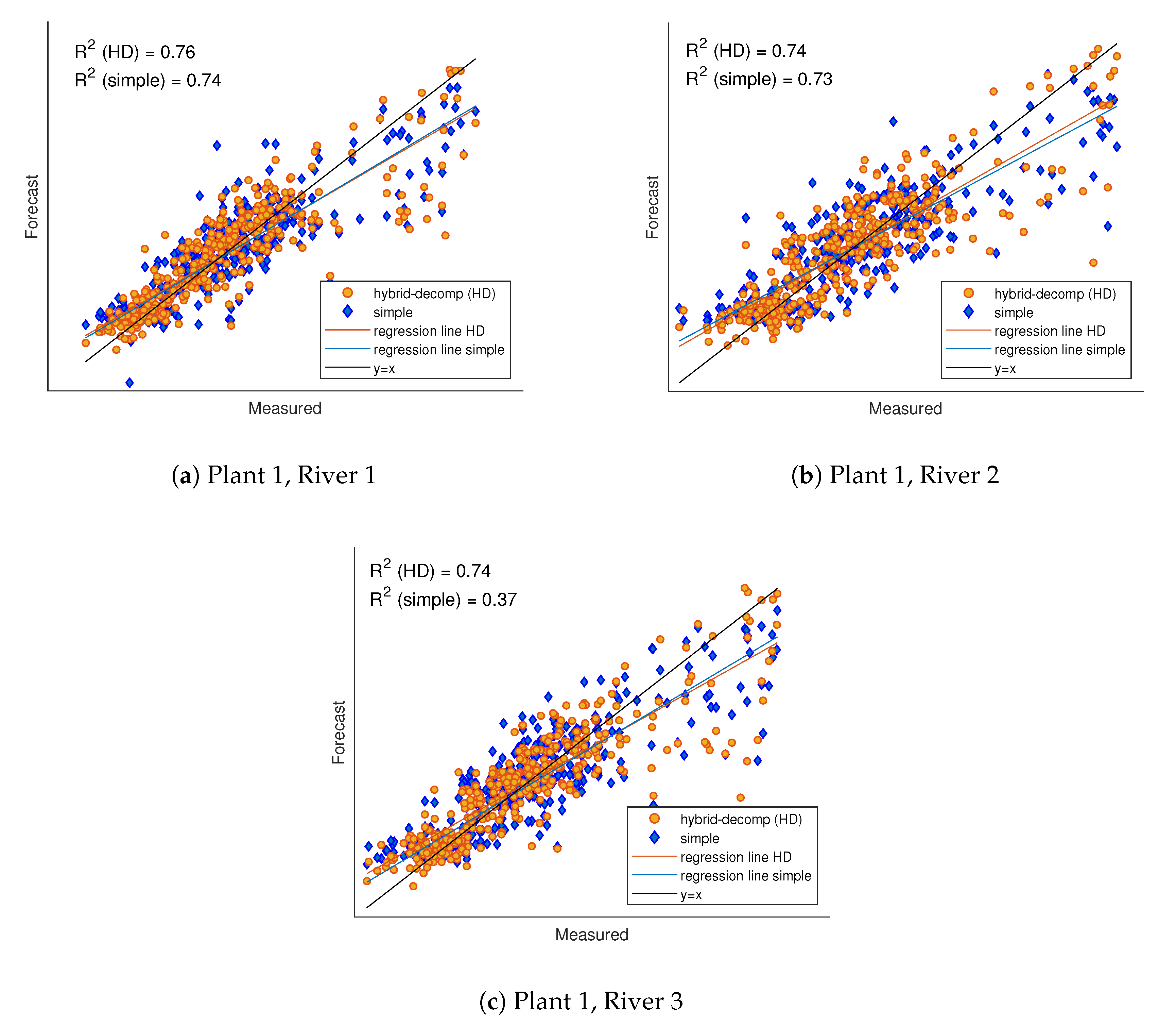
In Figure 10, the scatter plot related to the two approaches—hybrid with decomposition (orange dots) and ANN model (blue diamonds)—together with the associated regression lines (same colors) and the R 2 indicator, to evaluate the degree of accuracy of the forecast over the whole year are reported. In black it is drown the ideal regression line, in case of perfect forecast. On the x-axes is reported the measured production while on the y-axes is reported the forecast production. R 2 measures the goodness of the prediction: it reaches a maximum value of 1, and the closer it is to 1, the more the prediction can be considered precise.
The most distant points are always under the black line, in the right part of the chart, therefore the most relevant errors are made when the electric production is high, as the greater dispersion of the points in the top right highlights. Instead when production is low, as in the left part of the chart, the forecast reaches high levels of accuracy. This is maybe due to the low numerosity of observations of very high production. Indeed, for smaller values of measured power, it is possible to observe a lower dispersion of the points around the black line. In plant 1, River 1 (Figure 10a) and plant 1, River 3 (Figure 10c) the regression lines of the ANN and hybrid models almost coincide, while in plant 1, River 2 (Figure 10b) there is a small discrepancy in favor of the hybrid method. Focusing on the coefficient of determination R 2 , the hybrid decomposition values manage to better explain the variability in the measured data with respect to the ANN approach. The improvement is particularly significant for the plant 1, river 3, where the R 2 index doubles in the hybrid approach with respect to the benchmark case.

4. Conclusions

In this work, different approaches for daily hydroelectric production forecast, applied to fifteen RoR plants, along three different rivers, have been investigated. In particular it has been analyzed the effect, in terms of forecast accuracy, of diverse input data to the artificial neural network: sub-basins flow data derived from a hydrological model (HYPE) and precipitations data from three climate stations have been alternatively provided to a neural network in order to establish which can be more suitable for hydro-production forecast purposes. Furthermore the effect of production decomposition in its three components, trend, seasonality, and residual, has been analyzed. The hybrid approach, where precipitations are processed by the HYPE model to provide sub-basins flow as input to the ANN, outperformed the ANN model, both with and without decomposition. In addition, the hybrid forecast proved to be more performing than decomposed hybrid method in most of the analyzed plants.
Even if the presented case study is inherent to the RoR power plants, the current method could be adopted to other hydroelectric power plants characterized by the same features (seasonality, strong dependence on rainfalls and sub-basins flow, etc.).

Author Contributions

Conceptualization, E.O., A.N., M.M., S.P. and A.Z.; methodology, E.O., A.N. and M.M.; software, E.O., A.N. and M.M.; validation, A.N.; formal analysis, A.N. and E.O.; investigation, A.N.; data curation, A.N.; writing—original draft preparation, review and editing, A.N., E.O., M.M., S.P., A.Z., N.B. and M.A.; supervision, A.Z., M.A. and N.B. All authors have read and agreed to the published version of the manuscript.

Funding

This research received no external funding.

Conflicts of Interest

The authors declare no conflict of interest.

Abbreviations

The following abbreviations are used in this manuscript:
ANNArtificial Neural Network
ARIMAAuto Regressive Integrated Moving Average
CSBCorrelated Sub-Basins
ECAEuropean Climate Assessment
E f Nash–Sutcliffe Efficiency Index
HYPEHYdrological Predictions for the Environment
MAMoving Average
MAEMean Absolute Error
MASEMean Absolute Scaled Error
MBEMean Bias Error
PSPPumped Storage Plant
RoRRun of the River
SDStandard Deviation
SHPStorage Hydro Plants
SMAPESymmetric Mean Absolute Percentage Error
TSTime Series
TSOTransmission System Operator
TSSTraining Set Size

Appendix A

Table A1. Performance comparison: hybrid ANN with decomposition, hybrid ANN, ANN, and ANNs with decomposition.
(a) Plant 2, River 1.nMAEE f MASE
Hybrid + Dec.3.620.940.44
Hybrid3.510.940.43
ANN8.620.711.06
ANN + Dec.10.070.601.24
(b) Plant 3, River 1.nMAEE f MASE
Hybrid + Dec.5.270.870.58
Hybrid4.540.920.50
ANN9.510.721.05
ANN + Dec.12.990.441.43
(c) Plant 2, River 2.nMAEE f MASE
Hybrid + Dec.3.610.920.60
Hybrid3.230.940.54
ANN6.500.741.09
ANN + Dec.8.570.571.43
(d) Plant 3, River 2.nMAEE f MASE
Hybrid + Dec.3.740.930.61
Hybrid3.100.950.50
ANN6.790.721.11
ANN + Dec.9.210.611.50
(e) Plant 4, River 2.nMAEE f MASE
Hybrid + Dec.4.190.930.67
Hybrid3.630.930.58
ANN7.310.721.16
ANN + Dec.9.190.661.46
(f) Plant 5, River 2.nMAEE f MASE
Hybrid + Dec.4.070.930.62
Hybrid3.790.940.58
ANN7.110.761.09
ANN + Dec.9.420.681.44
(g) Plant 2, River 3.nMAEE f MASE
Hybrid + Dec.2.620.960.33
Hybrid2.780.930.35
ANN7.890.711.00
ANN + Dec.8.000.671.02
(h) Plant 3, River 3.nMAEE f MASE
Hybrid + Dec.2.630.960.34
Hybrid2.900.930.37
ANN7.600.720.97
ANN + Dec.7.590.680.97
(i) Plant 4, River 3.nMAEE f MASE
Hybrid + Dec.2.490.950.37
Hybrid2.700.940.40
ANN6.600.790.98
ANN + Dec.6.860.731.02
(j) Plant 5, River 3.nMAEE f MASE
Hybrid + Dec.2.550.960.41
Hybrid2.460.960.39
ANN6.390.791.02
ANN + Dec.6.650.711.07
(k) Plant 6, River 3.nMAEE f MASE
Hybrid + Dec.2.530.960.37
Hybrid2.780.930.40
ANN7.690.271.11
ANN + Dec.6.930.701.00
(l) Plant 7, River 3.nMAEE f MASE
Hybrid + Dec.2.320.960.34
Hybrid2.670.950.39
ANN7.010.711.03
ANN + Dec.7.020.711.03

References

  1. Giebel, G.; Al, E. The State of the Art in Short-Term Prediction of Wind Power. ANEMOS.Plus 2011, 1–110. [Google Scholar] [CrossRef]
  2. Mo, C.; Énergie, N.D.E.L.; Kim, Y.D.; Frei, C. World Energy Resources: Charting the Upsurge in Hydropower Development; World Energy Council: London, UK, 2015; p. 55. [Google Scholar]
  3. Levine, J.G. Pumped Hydroelectric Energy Storage and Spatial Diversity of Wind Resources as Methods of Improving Utilization of Renewable Energy Sources. Ph.D. Thesis, University of Colorado, Boulder, CO, USA, 2007. [Google Scholar]
  4. Resgaard, J.C. Hydrological Modelling and River Basin Management. Ph.D. Thesis, University of Copenhagen, Copenhagen, Denmark, 2007. [Google Scholar]
  5. Bergström, S. Development and Application of a Conceptual Runoff Model for Scandinavian Catchments. In Hydrologi Och Oceanografi, SMHI Reporter; Department of Water Resources Engineering, Lund Institute of Technology, University of Lund: Lund, Sweden, 1976; p. 134. [Google Scholar] [CrossRef]
  6. Arnold, J.G.; Fohrer, N. SWAT2000: Current capabilities and research opportunities in applied watershed modelling. Hydrol. Process. 2005, 19, 563–572. [Google Scholar] [CrossRef]
  7. Gupta, K.; Sharma, G.; Jethoo, A.; Tyagi, J.; Gupta, N. A critical review of hydrological models. In Proceedings of the 20th International Conference on Hydraulics, Water Resources and River Engineering, Roorkee, India, 17–19 December 2015; Volume 1, pp. 17–19. [Google Scholar]
  8. Islam, Z. Literature Review on Physically Based Hydrological Modeling; Technical Report February; University of Alberta: Edmonton, Alberta, 2011. [Google Scholar] [CrossRef]
  9. Dhami, B.S.; Pandey, A. Comparative Review of Recently Developed Hydrologic Models. J. Indian Water Resour. Soc. 2013, 33, 34–41. [Google Scholar]
  10. Solomatine, D.; See, L.M.; Abrahart, R.J. Approaches and Experiences. In Practical Hydroinformatics: Computational Intelligence and Technological Developments in Water Applications; Abrahart, R.J., See, L.M., Solomatine, D.P., Eds.; Springer: Berlin/Heidelberg, Germany, 2008; pp. 17–30. [Google Scholar] [CrossRef]
  11. De Menezes, M.L.; Teixeira Junior, L.A.; Morais De Souza, R.; Mara, C.K.; Moreira Pessanha, J.F.; Castro Souza, R. Hydroelectric energy forecast. Int. J. Energy Stat. 2013. [Google Scholar] [CrossRef]
  12. Mite-León, M.; Barzola-Monteses, J. Statistical model for the forecast of hydropower production in Ecuador. Int. J. Renew. Energy Res. 2018, 8, 1130–1137. [Google Scholar]
  13. Das, U.K.; Tey, K.S.; Seyedmahmoudian, M.; Mekhilef, S.; Idris, M.Y.I.; Van Deventer, W.; Horan, B.; Stojcevski, A. Forecasting of photovoltaic power generation and model optimization: A review. Renew. Sustain. Energy Rev. 2018, 81, 912–928. [Google Scholar] [CrossRef]
  14. Elshorbagy, A.; Corzo, G.; Srinivasulu, S.; Solomatine, D.P. Experimental investigation of the predictive capabilities of data driven modeling techniques in hydrology—Part 1: Concepts and methodology. Hydrol. Earth Syst. Sci. 2010, 14, 1931–1941. [Google Scholar] [CrossRef] [Green Version]
  15. Hammid, A.T.; Sulaiman, M.H.B.; Abdalla, A.N. Prediction of small hydropower plant power production in Himreen Lake dam (HLD) using artificial neural network. Alex. Eng. J. 2018, 57, 211–221. [Google Scholar] [CrossRef]
  16. Cobaner, M.; Haktanir, T.; Kisi, O. Prediction of Hydropower Energy Using ANN for the Feasibility of Hydropower Plant Installation to an Existing Irrigation Dam. Water Resour. Manag. 2008, 22, 757–774. [Google Scholar] [CrossRef]
  17. Beheshti, M.; Heidari, A.; Saghafian, B. Susceptibility of hydropower generation to climate change: Karun III Dam case study. Water 2019, 11, 1025. [Google Scholar] [CrossRef] [Green Version]
  18. Li, M.; Deng, C.H.; Tan, J.; Yang, W.; Zheng, L. Research on Small Hydropower Generation Forecasting Method Based on Improved BP Neural Network. In 2016 3rd International Conference on Materials Engineering, Manufacturing Technology and Control; Atlantis Press: Paris, France, 2016; pp. 1085–1090. [Google Scholar] [CrossRef] [Green Version]
  19. Monteiro, C.; Ramirez-Rosado, I.J.; Fernandez-Jimenez, L.A. Short-term forecasting model for electric power production of small-hydro power plants. Renew. Energy 2013, 50, 387–394. [Google Scholar] [CrossRef]
  20. Haykin, S. Neural Networks and Learning Machines, 3th ed.; Pearson: Upper Saddle River, NJ, USA, 2014. Available online: http://xxx.lanl.gov/abs/1312.6199v4 (accessed on 27 August 2020).
  21. Sobri, S.; Koohi-Kamali, S.; Rahim, N.A. Solar photovoltaic generation forecasting methods: A review. Energy Convers. Manag. 2018, 156, 459–497. [Google Scholar] [CrossRef]
  22. Escobar, R.; Antonanzas, J.; Antonanzas-Torres, F.; Urraca, R.; Osorio, N.; Martinez-de Pison, F. Review of photovoltaic power forecasting. Sol. Energy 2016, 136, 78–111. [Google Scholar] [CrossRef]
  23. Hussin, S.N.; Malek, M.A.; Jaddi, N.S.; Hamid, Z.A. Hybrid metaheuristic of artificial neural network-Bat algorithm in forecasting electricity production and water consumption at Sultan Azlan shah Hydropower plant. In Proceedings of the PECON 2016–2016 IEEE 6th International Conference on Power and Energy, Conference Proceeding, Melaka, Malaysia, 28–29 November 2016; pp. 28–31. [Google Scholar] [CrossRef]
  24. Wang, S.; Yu, L.; Tang, L.; Wang, S. A novel seasonal decomposition based least squares support vector regression ensemble learning approach for hydropower consumption forecasting in China. Energy 2011, 36, 6542–6554. [Google Scholar] [CrossRef]
  25. Zhang, H.; Singh, V.P.; Wang, B.; Yu, Y. CEREF: A hybrid data-driven model for forecasting annual streamflow from a socio-hydrological system. J. Hydrol. 2016, 540, 246–256. [Google Scholar] [CrossRef]
  26. Gaudard, L.; Avanzi, F.; De Michele, C. Seasonal aspects of the energy-water nexus: The case of a run-of-the-river hydropower plant. Appl. Energy 2018, 210, 604–612. [Google Scholar] [CrossRef]
  27. Wang, W.C.; Chau, K.W.; Xu, D.M.; Chen, X.Y. Improving Forecasting Accuracy of Annual Runoff Time Series Using ARIMA Based on EEMD Decomposition. Water Resour. Manag. 2015, 29, 2655–2675. [Google Scholar] [CrossRef]
  28. Zhang, G.P.; Qi, M. Neural network forecasting for seasonal and trend time series. Eur. J. Oper. Res. 2005, 160, 501–514. [Google Scholar] [CrossRef]
  29. Miller, D.M.; Williams, D. Shrinkage estimators of time series seasonal factors and their effect on forecasting accuracy. Int. J. Forecast. 2003, 19, 669–684. [Google Scholar] [CrossRef]
  30. Cleveland, W.P.; Tiao, G.C. Decomposition of Seasonal Time Series: A Model for the Census X-11 Program. J. Am. Stat. Assoc. 1976, 71, 581–587. [Google Scholar] [CrossRef]
  31. Sala, S.; Amendola, A.; Leva, S.; Mussetta, M.; Niccolai, A.; Ogliari, E. Comparison of Data-Driven Techniques for Nowcasting Applied to an Industrial-Scale Photovoltaic Plant. Energies 2019, 12, 4520. [Google Scholar] [CrossRef] [Green Version]
  32. Nespoli, A.; Ogliari, E.; Gavazzeni, M.; Vigani, S.; Paccanelli, F. Data quality analysis in day-ahead load forecast by means of LSTM. In Proceedings of the 2020 IEEE International Conference on Environment and Electrical Engineering and 2020 IEEE Industrial and Commercial Power Systems Europe (EEEIC/I&CPS Europe), Madrid, Spain, 9–12 June 2020. [Google Scholar]
  33. Lindström, G.; Pers, C.; Rosberg, J.; Strömqvist, J.; Arheimer, B. Development and testing of the HYPE (Hydrological Predictions for the Environment) water quality model for different spatial scales. Hydrol. Res. 2010, 41, 295–319. [Google Scholar] [CrossRef]
  34. Donnelly, C.; Andersson, J.C.M.; Arheimer, B. Using flow signatures and catchment similarities to evaluate the E-HYPE multi-basin model across Europe. Hydrol. Sci. J. 2016, 61, 255–273. [Google Scholar] [CrossRef]
  35. Strömqvist, J.; Arheimer, B.; Dahné, J.; Donnelly, C.; Lindström, G. Water and nutrient predictions in ungauged basins: Set-up and evaluation of a model at the national scale. Hydrol. Sci. J. 2012, 57, 229–247. [Google Scholar] [CrossRef] [Green Version]
  36. Arheimer, B.; Wallman, P.; Donnelly, C.; Nyström, K.; Arheimer, B.; Wallman, P.; Donnelly, C.; Nyström, K.; Pers, C. E-HypeWe: Service for Water and Climate Information and Future Hydrological Collaboration across Europe. In International Symposium on Environmental Software Systems; Springer: Berlin/Heidelberg, Germany, 2011; pp. 656–657. [Google Scholar]
  37. Andersson, J.C.M.; Pechlivanidis, I.G.; Gustafsson, D.; Donnelly, C.; Arheimer, B. Key factors for improving large-scale hydrological model performance. Eur. Water 2015, 49, 77–88. [Google Scholar]
  38. Montgomery, D.C.; Runger, G.C.; Hubele, N.F. Engineering Statistics, 5th ed.; John Wiley & Sons: Hoboken, NJ, USA, 2011. [Google Scholar]
  39. Adhikari, R. An Introductory Study on Time Series Modeling and Forecasting. 2013. Available online: http://xxx.lanl.gov/abs/1302.6613 (accessed on 29 August 2020).
  40. Tawfik, M. Linearity versus non-linearity in forecasting Nile River flows. Adv. Eng. Softw. 2003, 34, 515–524. [Google Scholar] [CrossRef]
  41. Da’Ar, O.B.; Ahmed, A.E. Underlying trend, seasonality, prediction, forecasting and the contribution of risk factors: An analysis of globally reported cases of Middle East Respiratory Syndrome Coronavirus. Epidemiol. Infect. 2018, 146, 1878. [Google Scholar] [CrossRef] [Green Version]
  42. Bashiri, M.; Farshbaf Geranmayeh, A. Tuning the parameters of an artificial neural network using central composite design and genetic algorithm. Sci. Iran. 2011, 18, 1600–1608. [Google Scholar] [CrossRef] [Green Version]
  43. Grimaccia, F.; Leva, S.; Mussetta, M.; Ogliari, E. ANN sizing procedure for the day-ahead output power forecast of a PV plant. Appl. Sci. 2017, 7, 622. [Google Scholar] [CrossRef] [Green Version]
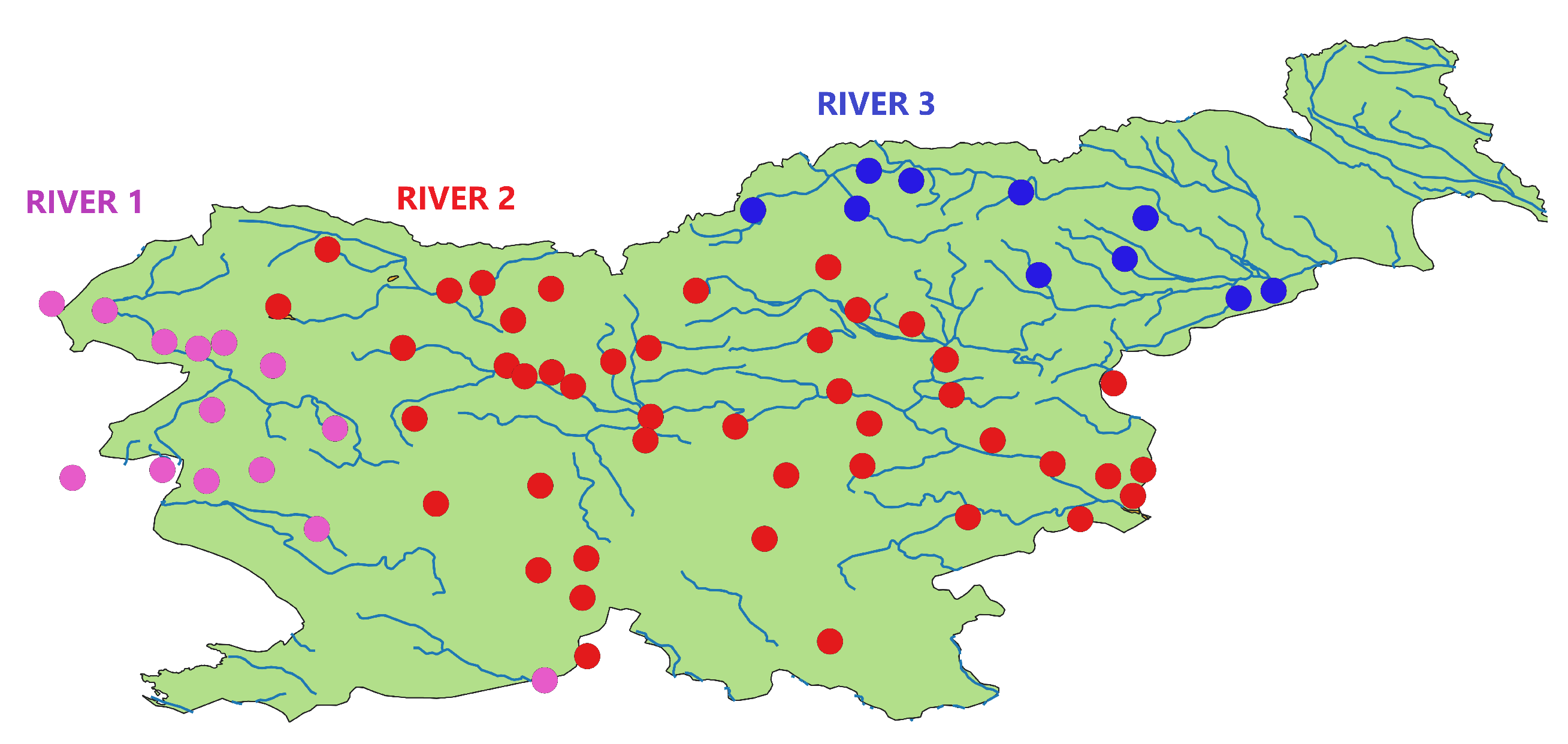
Figure 1. Sub-basins divided by river.
Forecasting 02 00022 g001
Figure 2. Hype schematic model.
Forecasting 02 00022 g002
Figure 3. Hybrid ANN training flow chart; CSB stands for Correlated Sub-Basins.
Forecasting 02 00022 g003
Figure 4. Hybrid ANN forecast flow chart; CSB stands for Correlated Sub-Basins.
Forecasting 02 00022 g004
Figure 5. Sensitivity analysis to select the number of days for the moving average computation.
Forecasting 02 00022 g005
Figure 6. Seasonal component of 3 plants on different rivers.
Forecasting 02 00022 g006
Figure 7. Production decomposition: observed, trend, seasonal, and residual power. X-axis indicates the day of the month from 9 May to 31 July.
Forecasting 02 00022 g007
Figure 8. Residual ANN structure for the hybrid approach of plant 2.
Forecasting 02 00022 g008
Figure 9. Comparison between forecast (red) and observed (blue) values in the decomposition phases: (a) Trend component; (b) Residual Component; (c) Recomposed production (Trend, Seasonality and Residual).
Forecasting 02 00022 g009
Figure 10. Scatterplot comparison, obtained with real data on x-axis and forecast data on y-axis. In blue the results got with the hybrid decomposition approach, in orange the results with the ANN model for three of the considered plants: (a) Plant 1 on river 1; (b) Plant 1 on river 2; (c) Plant 1 on river 3.
Forecasting 02 00022 g010
Table 1. Hybrid ANN parameters settings; TSS is the Training Set Size.
Decomposition-TrendDecomposition-Resididual
TSS [ d a y s ] 50100
N. Layers12
N. Neurons84,4
N. Inputs6 + N of CSB7 + N of CSB
Input LayerCSB ( ρ > 0.5),CSB ( ρ > 0.5),
W o b s past 6 days W o b s past 6 days, trend forecast
Output Layertrend forecastresidual forecast
Table 2. Benchmark ANNs parameters settings: Hybrid, ANN, and ANNs with decomposition (Trend and Residual); TSS is the Training Set Size.
HybridANNANN + Dec.-TrendANN + Dec.-Resididual
TSS [ d a y s ] 25025050100
N. Layers1112
N. Neurons12466,3
N. Inputs6 + N of CSB9910
Input LayerCSB ( ρ > 0.5),precipitation [mm],precipitation [mm],precipitation [mm],
W o b s past 6 days W o b s past 6 days W o b s past 6 days W o b s past 6 days, trend forecast
Output Layerproduction forecastproduction forecasttrend forecastresidual forecast
Table 3. Performance comparison proposed method and the three benchmarks considered: Hybrid with decomposition, Hybrid, ANN, and ANNs with decomposition for three of the analyzed plants: (a) plant 1 on river 1, (b) plant 1 on river 2 and (c) plant 1 on river 3. Color legend from the best to the worst result: green, olive, orange, and magenta.
(a) Plant 1, River 1.nMAEE f MASE
Hybrid + Dec.4.750.910.61
Hybrid3.890.940.50
ANN8.180.721.04
ANN + Dec.10.940.571.40
(b) Plant 1, River 2.nMAEE f MASE
Hybrid + Dec.3.680.870.72
Hybrid2.970.920.58
ANN5.530.711.08
ANN + Dec.7.840.471.53
(c) Plant 1, River 3.nMAEE f MASE
Hybrid + Dec.2.520.960.39
Hybrid2.560.960.40
ANN6.790.651.04
ANN + Dec.6.830.691.05
Table 4. Mean performance and standard deviation (SD) of the methods under analysis: (a) and (b) refer to River 1, (c) and (d) refer to River 2, (e) and (f) refer to River 3 while (g) and (h) report mean and standard deviation of all the plants together.
(a) Mean Plants on River 1.nMAEE f MASE
Hybrid + Dec.3.860.920.64
Hybrid3.340.940.56
ANN6.650.731.10
ANN + Dec.8.850.601.47
(b) SD Plants on River 1.nMAEE f MASE
Hybrid + Dec.0.250.030.05
Hybrid0.350.010.03
ANN0.700.020.03
ANN + Dec.0.650.080.04
(c) Mean Plants on River 2.nMAEE f MASE
Hybrid + Dec.4.550.910.54
Hybrid3.980.930.48
ANN8.770.721.05
ANN + Dec.11.330.531.35
(d) SD Plants on River 2.nMAEE f MASE
Hybrid + Dec.0.840.030.09
Hybrid0.520.010.40
ANN0.680.010.01
ANN + Dec.1.500.080.11
(e) Mean Plants on River 3.nMAEE f MASE
Hybrid + Dec.2.520.960.36
Hybrid2.700.940.39
ANN7.140.661.02
ANN + Dec.7.130.701.02
(f) SD Plants on River 3.nMAEE f MASE
Hybrid + Dec.0.100.010.03
Hybrid0.140.010.02
ANN0.590.180.05
ANN + Dec.0.490.020.03
(g) Mean All PlantsnMAEE f MASE
Hybrid + Dec.3.370.930.49
Hybrid3.170.940.46
ANN7.300.701.06
ANN + Dec.8.540.631.24
(h) SD All Plants.nMAEE f MASE
Hybrid + Dec.0.930.030.14
Hybrid0.590.010.08
ANN0.990.120.05
ANN + Dec.1.800.090.22
Publisher’s Note: MDPI stays neutral with regard to jurisdictional claims in published maps and institutional affiliations.