Forecasting of Future Flooding and Risk Assessment under CMIP6 Climate Projection in Neuse River, North Carolina


Abstract
1. Introduction
- (a)
- What would be the impact of climate change on future streamflow, and how will it affect the flood frequency?
- (b)
- Under the projected design discharge, what would be the future change in flood extent and patterns?
- (c)
- By what times would the future flood risk increase under the climate change scenarios compared to existing FEMA scenario?
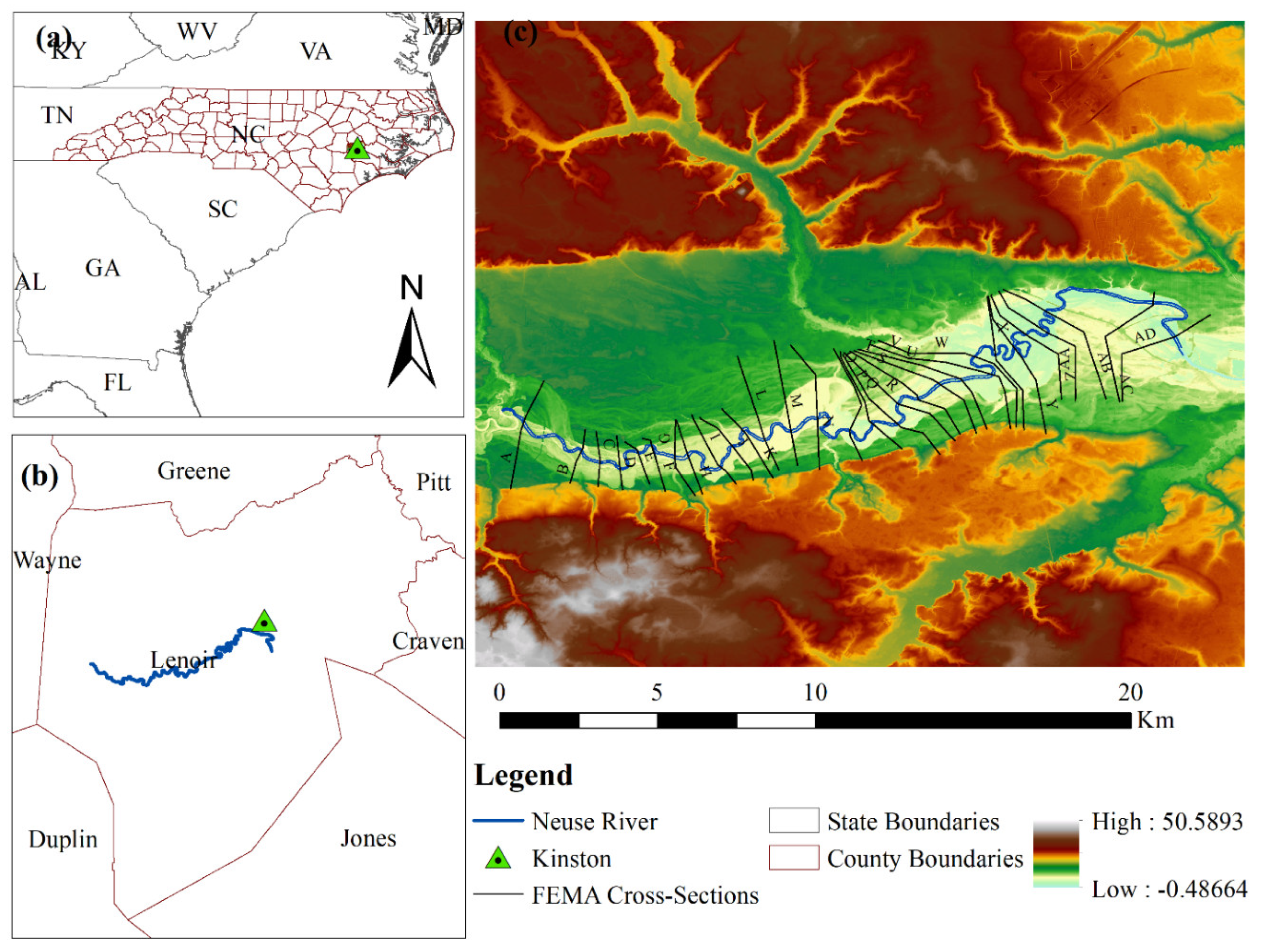
2. Study Area and Data Used
2.1. Study Area
2.2. Dataset
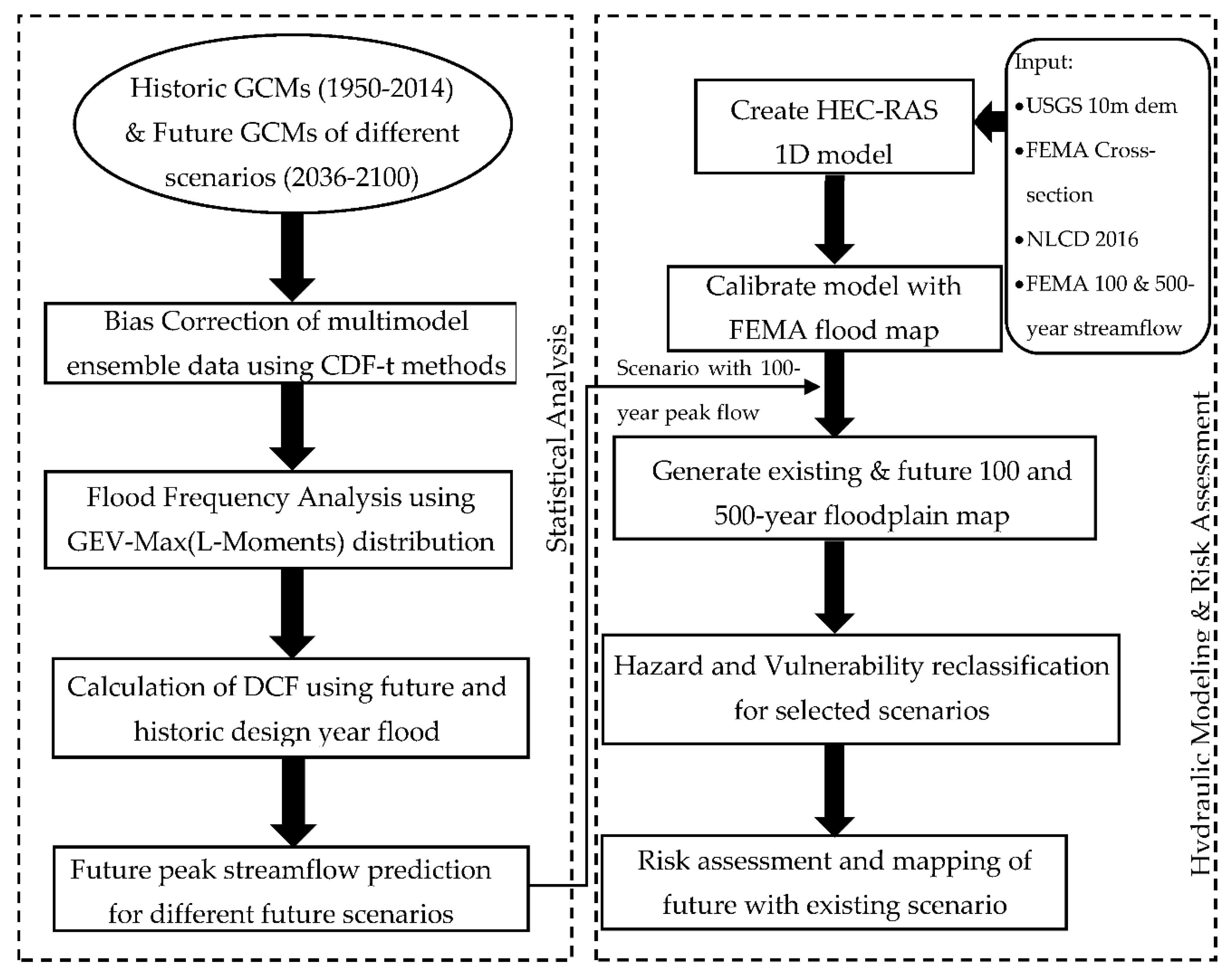
3. Methods
3.1. Statistical Analysis
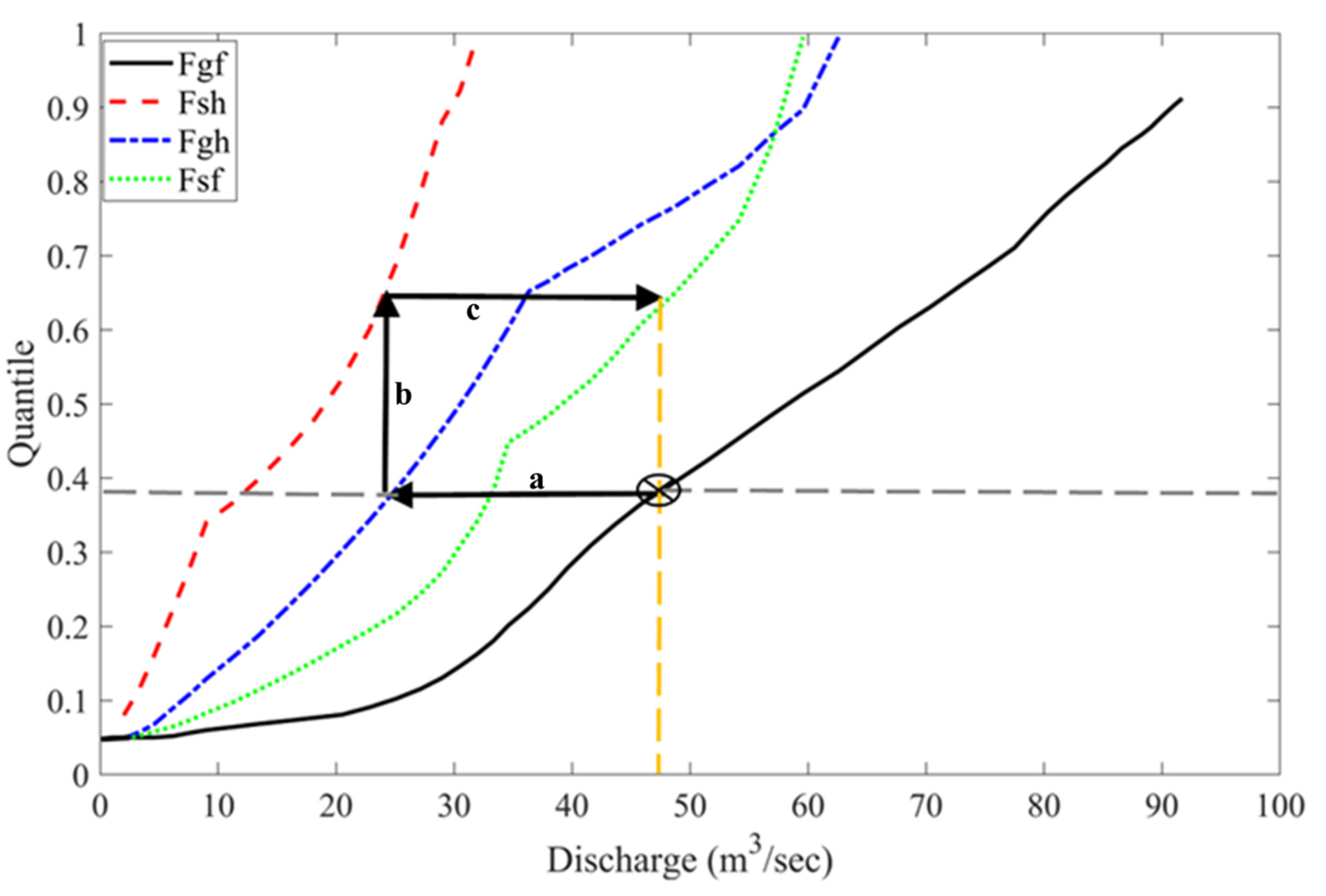
3.1.1. Bias Correction
3.1.2. Quantification of the Future Design Flow
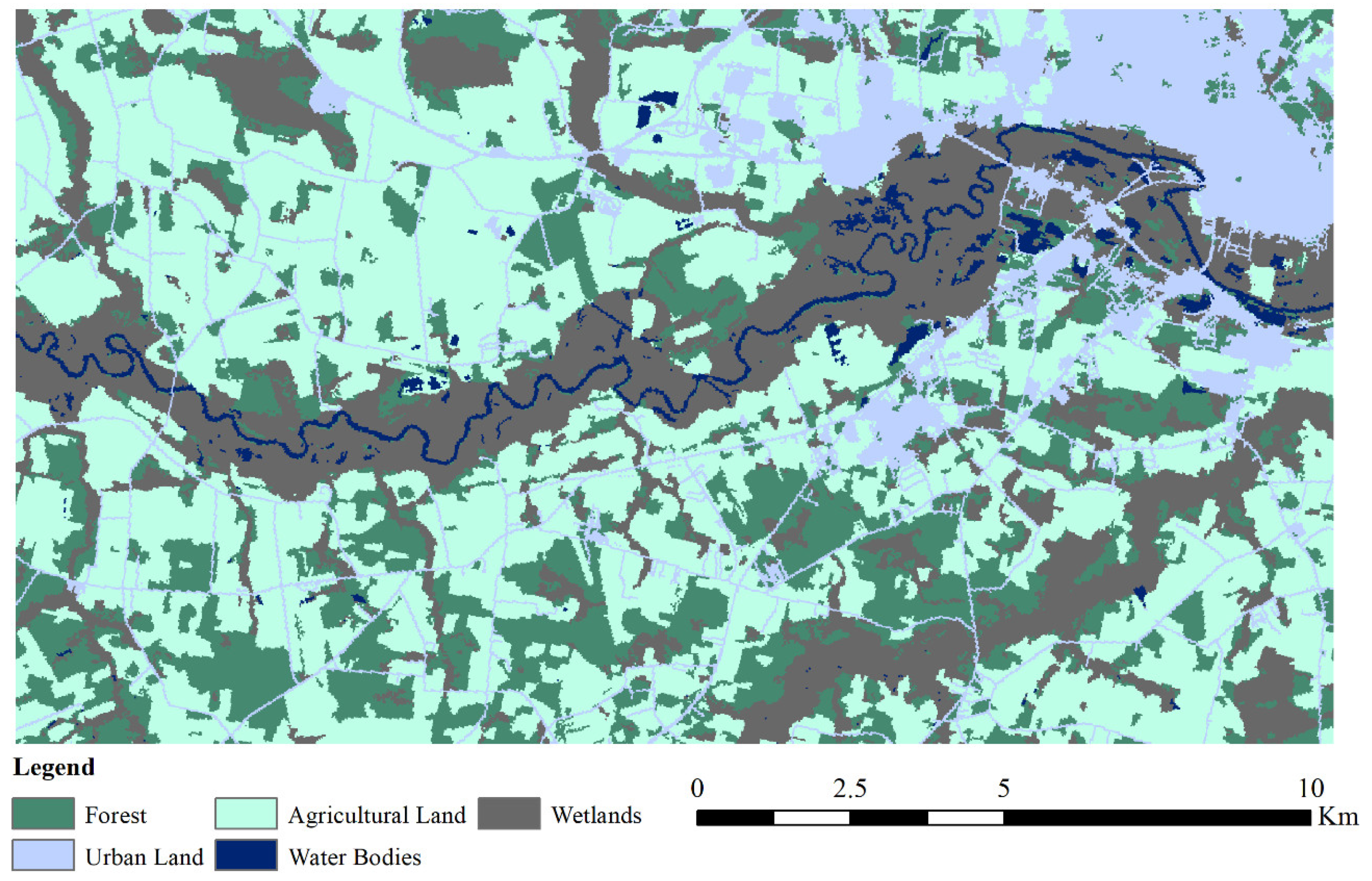
3.2. Hydraulic Modeling and Risk Assessment Classification
4. Results
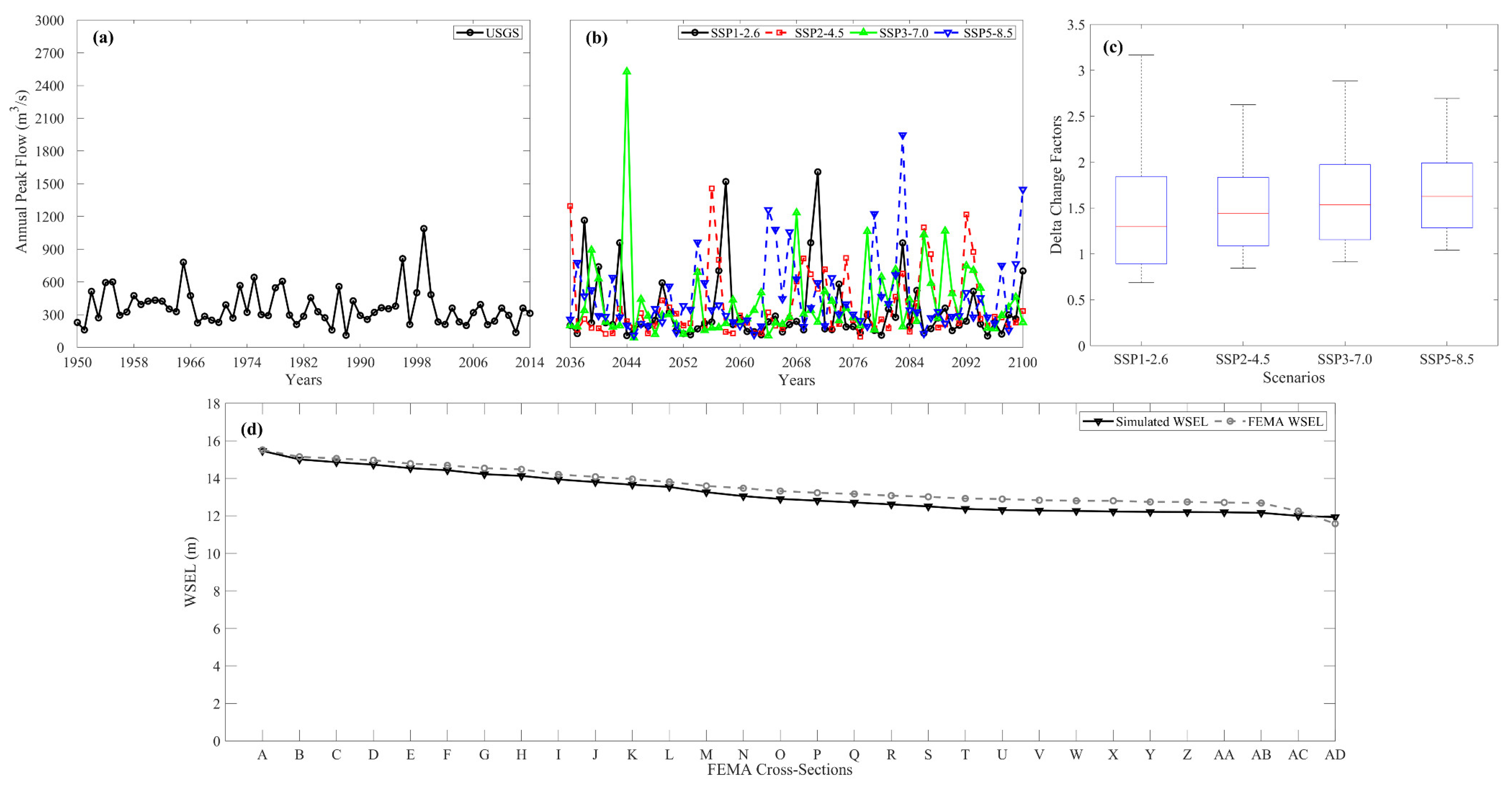
4.1. Flood Frequency Analysis and Performance of Hydraulic Modeling
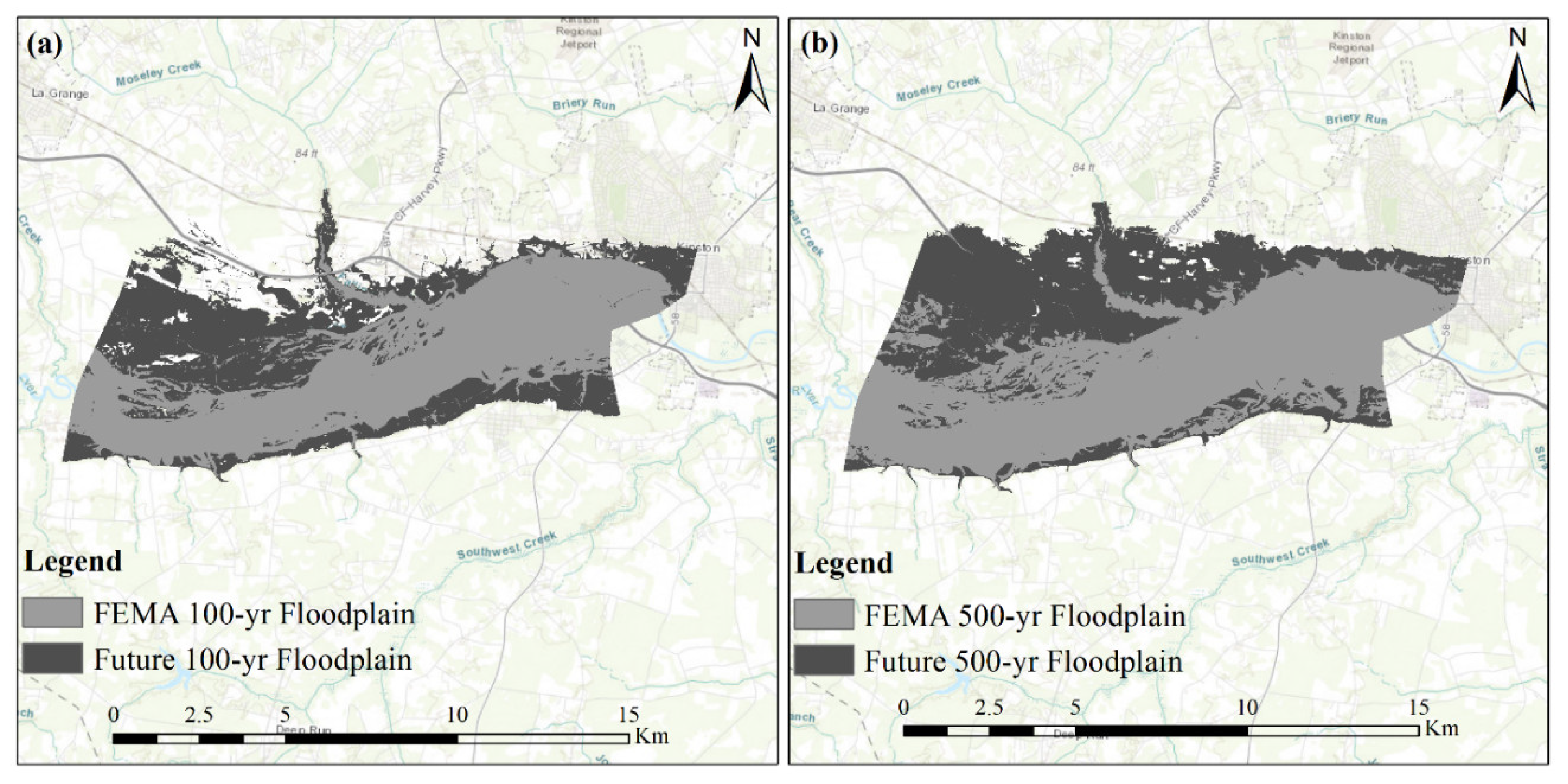
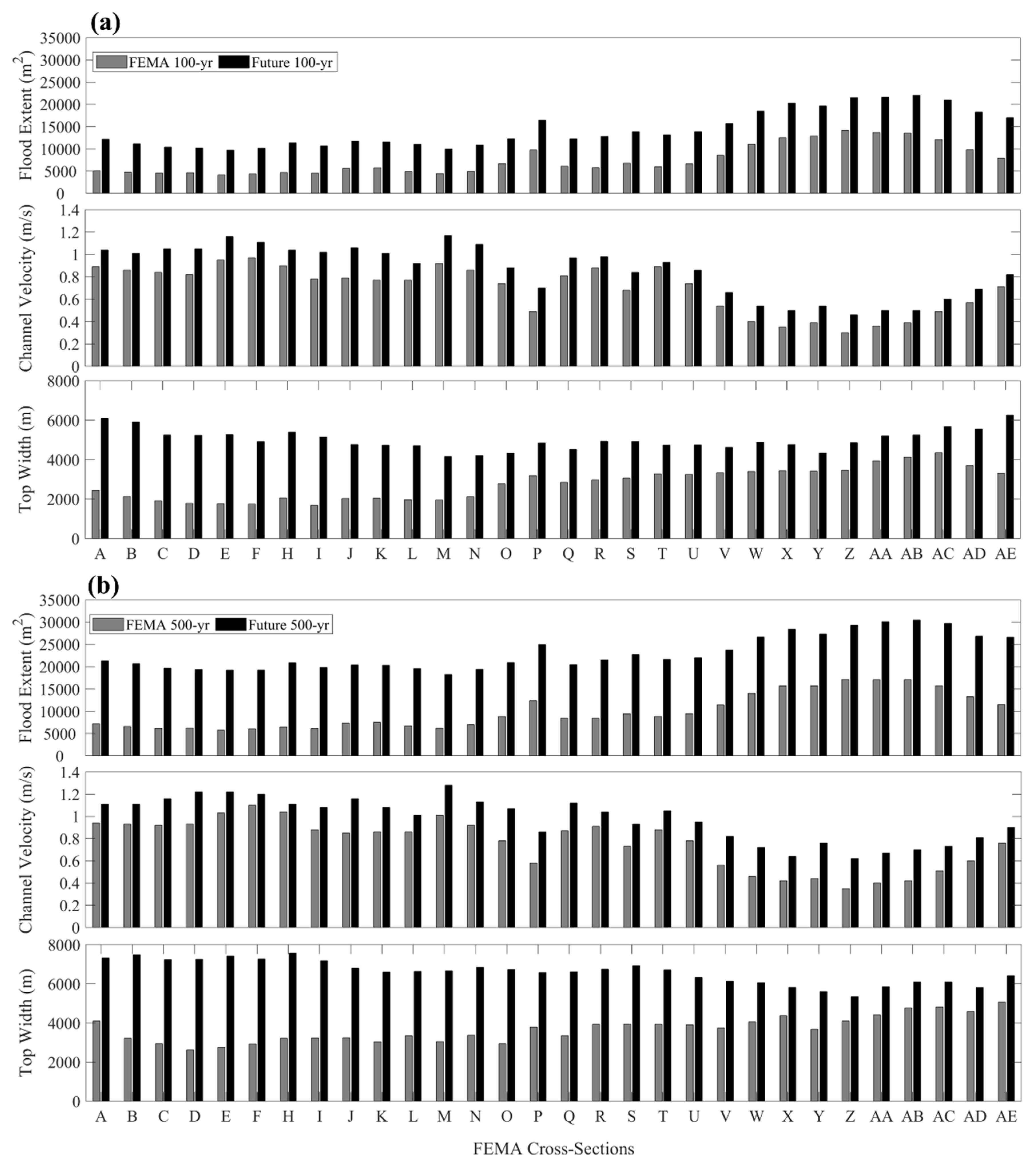
4.2. Flood Inundation Mapping
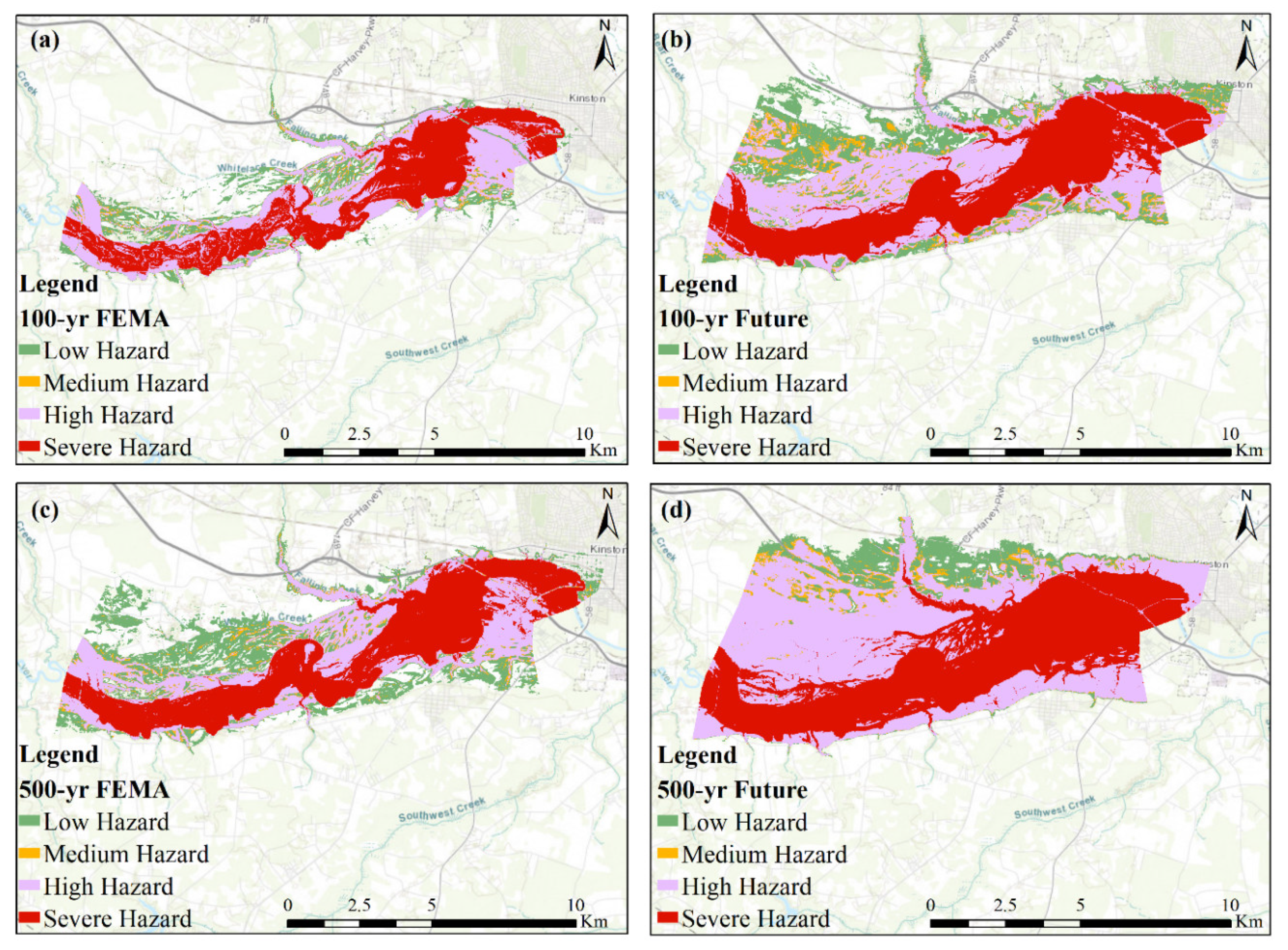
4.3. Flood Hazard Assessment
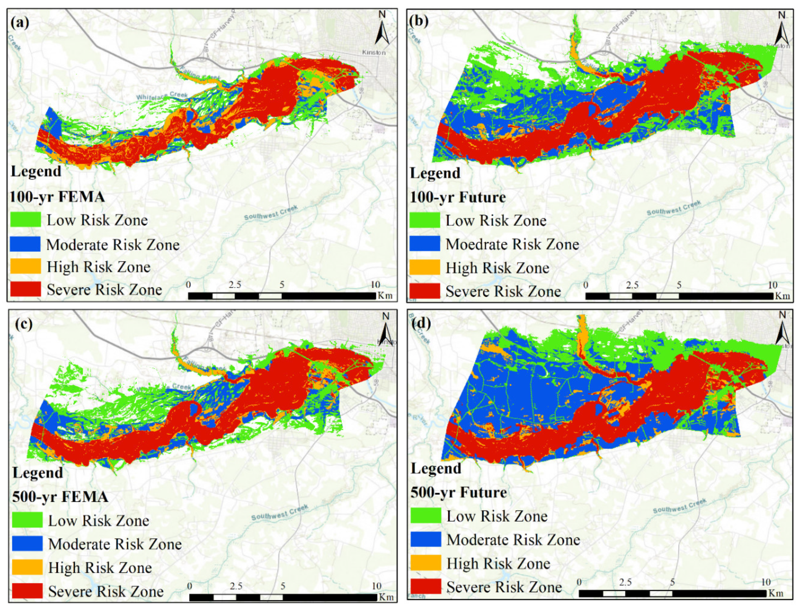
4.4. Risk Zone Assessment and Mapping
5. Discussion
6. Conclusions
- Bias correction of different scenarios obtained from the multimodel ensemble with the historical data was performed using the CDF-t method. The CDF-t method increases the robustness in evaluating future change in streamflow.
- For the estimation of the design flow, GEV-Max (L-Moments) was utilized, where SSP5-8.5 was found to have a maximum flow for the 100-year return period.
- The DCF for most future scenarios were found to be higher than 1, suggesting the increase in future streamflow in comparison with the existing (FEMA) flow.
- For the 100-year return period flood event, future scenario SSP5-8.5 predicted the maximum increase in the peak flow in Neuse River.
- HEC-RAS 1D steady modeling was used to simulate the floodplain mapping extent of Neuse River, NC. The result showed a higher extent of flooding for the future 100-year scenario than for the existing FEMA 500-year peak flows.
- Reclassification and mapping of hazard, vulnerability, and risk were completed utilizing the SSP5-8.5 scenario for the assessment of risk.
- The extent of different flood risk zone of future flows for 100 and 500-year flood events highlights the increase in potential risk and their severity in the future.
Author Contributions
Funding
Acknowledgments
Conflicts of Interest
References
- Allen, R.M.; Dube, O.P.; Solecki, W.; Aragon-Durand, F.; Cramer, W.; Humphreys, S.; Kainuma, M.; Kala, J.; Mahowald, N.; Mulugetta, Y.; et al. Framing and context. In Global Warming of 1.5 °C. An IPCC Special Report on the Impacts of Global Warming of 1.5 °C above Pre-Industrial Levels and Related Global Greenhouse Gas Emission Pathways, in the Context of Strengthening the Global Response to the Threat of Climate Change, Sustainable Development, and Efforts to Eradicate Poverty; Masson-Delmotte, V.P., Zhai, H.-O., Portner, D., Roberts, J., Skea, P.R., Shukla, A., Pirani, W., Moufouma-Okia, C., Pean, R., Pidcock, S., et al., Eds.; Intergovernmental Panel on Climate Change: Geneva, Switzerland, 2018; in press. [Google Scholar]
- Merz, B.; Aerts, J.; Arnbjerg-Nielsen, K.; Baldi, M.; Becker, A.; Bichet, A.; Blöschl, G.; Bouwer, L.M.; Brauer, A.; Cioffi, F.; et al. Floods and climate: Emerging perspectives for flood risk assessment and management. NHESS 2014, 14, 1921–1942. [Google Scholar] [CrossRef]
- Easterling, D.R.; Meehl, G.A.; Parmesan, C.; Changnon, S.A.; Karl, T.R.; Mearns, L.O. Climate extremes: Observations, modeling, and impacts. Science 2000, 289, 2068–2074. [Google Scholar] [CrossRef]
- Griffin, M.T.; Montz, B.E.; Arrigo, J.S. Evaluating climate change induced water stress: A case study of the lower cape fear basin, NC. Appl. Geogr. 2013, 40, 115–128. [Google Scholar] [CrossRef]
- Middelkoop, H.; Daamen, K.; Gellens, D.; Grabs, W.; Kwadijk, J.C.; Lang, H.; Wilke, K. Impact of climate change on hydrological regimes and water resources management in the Rhine basin. Clim. Chang. 2001, 49, 105–128. [Google Scholar] [CrossRef]
- Roy, L.; Leconte, R.; Brissette, F.P.; Marche, C. The impact of climate change on seasonal floods of a southern Quebec River Basin. Hydrol. Process. 2001, 15, 3167–3179. [Google Scholar] [CrossRef]
- Arnell, N.W.; Gosling, S.N. The impacts of climate change on river flood risk at the global scale. Clim. Chang. 2016, 134, 387–401. [Google Scholar] [CrossRef]
- Hirabayashi, Y.; Kanae, S.; Emori, S.; Oki, T.; Kimoto, M. Global projections of changing risks of floods and droughts in a changing climate. Hydrol. Sci. J. 2008, 53, 754–772. [Google Scholar] [CrossRef]
- De Paola, F.; Giugni, M.; Pugliese, F.; Annis, A.; Nardi, F. GEV parameter estimation and stationary vs. non-stationary analysis of extreme rainfall in African test cities. Hydrology 2018, 5, 28. [Google Scholar] [CrossRef]
- Alfieri, L.; Feyen, L.; Dottori, F.; Bianchi, A. Ensemble flood risk assessment in Europe under high end climate scenarios. Glob. Environ. Chang. 2015, 35, 199–212. [Google Scholar] [CrossRef]
- Bhandari, R.; Kalra, A.; Kumar, S. Analyzing the effect of CMIP5 climate projections on streamflow within the Pajaro River Basin. Water J. 2020, 6, 5. [Google Scholar]
- Chattopadhyay, S.; Jha, M.K. Hydrological response due to projected climate variability in Haw River watershed, North Carolina, USA. Hydrol. Sci. J. 2016, 61, 495–506. [Google Scholar] [CrossRef]
- Johnson, T.; Butcher, J.; Deb, D.; Faizullabhoy, M.; Hummel, P.; Kittle, J.; Sarkar, S. Modeling streamflow and water quality sensitivity to climate change and urban development in 20 US watersheds. JAWRA J. Am. Water. Resour. Assoc. 2015, 51, 1321–1341. [Google Scholar] [CrossRef]
- Arnell, N.W. Climate change and global water resources. Glob. Environ. Chang. 1999, 9, S31–S49. [Google Scholar] [CrossRef]
- Hall, K. Expected Costs of Damage from Hurricane Winds and Storm-Related Flooding; Congressional Budget Office: Washington, DC, USA, 2019; pp. 1–48. [Google Scholar]
- Guidance of Flood Risk Analysis and Mapping; Hydraulics: One-Dimensional Analysis. Available online: https://www.fema.gov/media-library-data/1484864685338-42d21ccf2d87c2aac95ea1d7ab6798eb/Hydraulics_OneDimensionalAnalyses_Nov_2016.pdf (accessed on 3 January 2020).
- Brunner, G.W. HEC-RAS, River Analysis System Hydraulic Reference Manual, Version 5.0; US Army Corps of Engineers: Davis, CA, USA, 2016; pp. 3–538. [Google Scholar]
- Joshi, N.; Lamichhane, G.R.; Rahaman, M.M.; Kalra, A.; Ahmad, S. Application of HEC-RAS to Study the Sediment Transport Characteristics of Maumee River in Ohio; World Environmental and Water Resources Congress: Reston, VA, USA, 2019; pp. 257–267. [Google Scholar]
- Yang, J.; Townsend, R.D.; Daneshfar, B. Applying the HEC-RAS model and GIS techniques in river network floodplain delineation. Can. J. Civil. Eng. 2006, 33, 19–28. [Google Scholar] [CrossRef]
- Lim, N.J. Performance and Uncertainty Estimation of 1-and 2-Dimensional Flood Models. Master’s Thesis, University of Gävle, Gävle, Sweden, June 2011. [Google Scholar]
- ShahiriParsa, A.; Noori, M.; Heydari, M.; Rashidi, M. Floodplain zoning simulation by using HEC-RAS and CCHE2D models in the Sungai Maka river. Sage Open. 2016, 9. [Google Scholar] [CrossRef]
- Mehta, D.J.; Ramani, M.M.; Joshi, M.M. Application of 1-D HEC-RAS model in design of channels. Methodology 2013, 1, 4–62. [Google Scholar]
- Peng, A.; Liu, F. Flooding simulation due to hurricane florence in North Carolina with HEC RAS. arXiv 2019, arXiv:1911.09525. [Google Scholar]
- Bathi, J.R.; Das, H.S. Vulnerability of coastal communities from storm surge and flood disasters. Int. J. Environ. Res. Public Health 2016, 13, 239. [Google Scholar] [CrossRef]
- Tingsanchali, T.; Karim, F. Flood-hazard assessment and risk-based zoning of a tropical flood plain: Case study of the Yom River, Thailand. Hydrol. Sci. J. 2010, 55, 145–161. [Google Scholar] [CrossRef]
- Mihu-Pintilie, A.; Cîmpianu, C.I.; Stoleriu, C.C.; Pérez, M.N.; Paveluc, L.E. Using high-density LiDAR Data and 2D streamflow hydraulic modeling to improve urban flood hazard maps: A HEC-RAS multi-scenario approach. Water 2019, 11, 1832. [Google Scholar] [CrossRef]
- Klijn, F.; Kreibich, H.; De Moel, H.; Penning-Rowsell, E. Adaptive flood risk management planning based on a comprehensive flood risk conceptualisation. Mitig. Adapt. Strateg. Glob. Chang. 2015, 20, 845–864. [Google Scholar] [CrossRef]
- Tingsanchali, T.; Karim, M.F. Flood hazard and risk analysis in the southwest region of Bangladesh. Hydrol. Process. 2005, 19, 2055–2069. [Google Scholar] [CrossRef]
- Noren, V.; Hedelin, B.; Nyberg, L.; Bishop, K. Flood risk assessment–practices in flood prone Swedish municipalities. Int. J. Disaster. Risk Reduct. 2016, 18, 206–217. [Google Scholar] [CrossRef]
- Eyring, V.; Bony, S.; Meehl, G.A.; Senior, C.A.; Stevens, B.; Stouffer, R.J.; Taylor, K.E. Overview of the Coupled Model Intercomparison Project Phase 6 (CMIP6) experimental design and organization. Geosci. Model Dev. 2016, 9, 1937–1958. [Google Scholar] [CrossRef]
- Meehl, G.A.; Moss, R.; Taylor, K.E.; Eyring, V.; Stouffer, R.J.; Bony, S.; Stevens, B. Climate model intercomparisons: Preparing for the next phase. Eos Trans. Am. Geophys. Union 2014, 95, 77–78. [Google Scholar] [CrossRef]
- Riahi, K.; Van Vuuren, D.P.; Kriegler, E.; Edmonds, J.; O’neill, B.C.; Fujimori, S.; Lutz, W. The shared socioeconomic pathways and their energy, land use, and greenhouse gas emissions implications: An overview. Glob. Environ. Chang. 2017, 42, 153–168. [Google Scholar] [CrossRef]
- Stouffer, R.J.; Eyring, V.; Meehl, G.A.; Bony, S.; Senior, C.; Stevens, B.; Taylor, K.E. CMIP5 scientific gaps and recommendations for CMIP6. Bull. Am. Meteorol. Soc. 2017, 98, 95–105. [Google Scholar] [CrossRef]
- O’Neill, B.C.; Tebaldi, C.; Van Vuuren, D.P.; Eyring, V.; Friedlingstein, P.; Hurtt, G.; Meehl, G.A. The scenario model intercomparison project (ScenarioMIP) for CMIP6. Geosci. Model Dev. 2016, 9, 3461–3482. [Google Scholar] [CrossRef]
- Joshi, N.; Tamaddun, K.; Parajuli, R.; Kalra, A.; Maheshwari, P.; Mastino, L.; Velotta, M. Future changes in water supply and demand for Las Vegas valley: A system dynamic approach based on CMIP3 and CMIP5 climate projections. Hydrology 2020, 7, 16. [Google Scholar] [CrossRef]
- Moradkhani, H.; Baird, R.G.; Wherry, S.A. Assessment of climate change impact on floodplain and hydrologic ecotones. J. Hydrol. 2010, 395, 264–278. [Google Scholar] [CrossRef]
- Alfieri, L.; Bisselink, B.; Dottori, F.; Naumann, G.; de Roo, A.; Salamon, P.; Wyser, K.; Feyen, L. Global projections of river flood risk in a warmer world. Earths Future 2017, 5, 171–182. [Google Scholar] [CrossRef]
- Shrestha, A.; Rahaman, M.M.; Kalra, A.; Jogineedi, R.; Maheshwari, P. Climatological drought forecasting using bias corrected CMIP6 climate data: A case study for India. Forecasting 2020, 2, 4. [Google Scholar] [CrossRef]
- Stevenson, D.S.; Dentener, F.J.; Schultz, M.G.; Ellingsen, K.; Van Noije, T.P.C.; Wild, O.; Bergmann, D.J. Multimodel ensemble simulations of present-day and near-future tropospheric ozone. J. Geophys. Res. Atmos. 2006, 111. [Google Scholar] [CrossRef]
- Nohara, D.; Kitoh, A.; Hosaka, M.; Oki, T. Impact of climate change on river discharge projected by multimodel ensemble. J. Hydrometeorol. 2006, 7, 1076–1089. [Google Scholar] [CrossRef]
- Nam, D.H.; Udo, K.; Mano, A. Future fluvial flood risks in C entral V ietnam assessed using global super-high-resolution climate model output. J. Flood Risk Manag. 2015, 8, 276–288. [Google Scholar] [CrossRef]
- Kay, A.L.; Davies, H.N.; Bell, V.A.; Jones, R.G. Comparison of uncertainty sources for climate change impacts: Flood frequency in England. Clim. Chang. 2009, 92, 41–63. [Google Scholar] [CrossRef]
- Christensen, J.H.; Boberg, F.; Christensen, O.B.; Lucas-Picher, P. On the need for bias correction of regional climate change projections of temperature and precipitation. Geophys. Res. Lett. 2008, 35. [Google Scholar] [CrossRef]
- Nyaupane, N.; Thakur, B.; Kalra, A.; Ahmad, S. Evaluating future flood scenarios using CMIP5 climate projections. Water 2018, 10, 1866. [Google Scholar] [CrossRef]
- Wang, L.; Chen, W. Equiratio cumulative distribution function matching as an improvement to the equidistant approach in bias correction of precipitation. Atmos. Sci. Lett. 2014, 15, 1–6. [Google Scholar] [CrossRef]
- Salvi, K.; Kannan, S.; Ghosh, S. Statistical downscaling and bias-correction for projections of Indian rainfall and temperature in climate change studies. In Proceedings of the 4th International Conference on Environmental and Computer Science, Singapore, 2–4 September 2011; pp. 16–18. [Google Scholar]
- Mishra, B.K.; Rafiei Emam, A.; Masago, Y.; Kumar, P.; Regmi, R.K.; Fukushi, K. Assessment of future flood inundations under climate and land use change scenarios in the Ciliwung River Basin, Jakarta. J. Flood Risk Manag. 2018, 11, S1105–S1115. [Google Scholar] [CrossRef]
- Cannon, A.J.; Sobie, S.R.; Murdock, T.Q. Bias correction of GCM precipitation by quantile mapping: How well do methods preserve changes in quantiles and extremes? J. Clim. 2015, 28, 6938–6959. [Google Scholar] [CrossRef]
- Camici, S.; Brocca, L.; Melone, F.; Moramarco, T. Impact of climate change on flood frequency using different climate models and downscaling approaches. J. Hydrol. Eng. 2014, 19, 04014002. [Google Scholar] [CrossRef]
- Guo, L.Y.; Gao, Q.; Jiang, Z.H.; Li, L. Bias correction and projection of surface air temperature in LMDZ multiple simulation over central and eastern China. Adv. Clim. Chang. Res. 2018, 9, 81–92. [Google Scholar] [CrossRef]
- Michelangeli, P.A.; Vrac, M.; Loukos, H. Probabilistic downscaling approaches: Application to wind cumulative distribution functions. Geophys. Res. Lett. 2009, 36. [Google Scholar] [CrossRef]
- Pierce, D.W.; Cayan, D.R.; Maurer, E.P.; Abatzoglou, J.T.; Hegewisch, K.C. Improved bias correction techniques for hydrological simulations of climate change. J. Hydrometeorol. 2015, 16, 2421–2442. [Google Scholar] [CrossRef]
- Famien, A.M.; Janicot, S.; Ochou, A.D.; Vrac, M.; Defrance, D.; Sultan, B.; Noel, T. A bias-corrected CMIP5 dataset for Africa using the CDF-t method: A contribution to agricultural impact studies. Earth Syst. Dynam. 2018, 9, 313–338. [Google Scholar] [CrossRef]
- Yuan, X.; Wood, E.F. Downscaling precipitation or bias-correcting streamflow? Some implications for coupled general circulation model (CGCM)-based ensemble seasonal hydrologic forecast. Water Resour. Res. 2012, 48. [Google Scholar] [CrossRef]
- Hamzah, F.M.; Yusoff, S.H.M.; Jaafar, O. L-moment-based frequency analysis of high-flow at Sungai Langat, Kajang, Selangor, Malaysia. Sains Malays. 2019, 48, 1357–1366. [Google Scholar] [CrossRef]
- Teegavarapu, R.S.; Pathak, C.S. Statistical analysis of precipitation extremes. In Statistical Analysis of Hydrologic Variables: Methods and Applications; American Society of Civil Engineering: Reston, VA, USA, 2019; pp. 5–70. [Google Scholar]
- Ayuketang Arreyndip, N.; Joseph, E. Generalized extreme value distribution models for the assessment of seasonal wind energy potential of Debuncha, Cameroon. J. Renew. Energy 2016, 2016, 9. [Google Scholar] [CrossRef]
- Hosking, J.R.M.; Wallis, J.R.; Wood, E.F. Estimation of the generalized extreme-value distribution by the method of probability-weighted moments. Technometrics 1985, 27, 251–261. [Google Scholar] [CrossRef]
- Santos, E.B.; Lucio, P.S.; e Silva, C.M.S. Estimating return periods for daily precipitation extreme events over the Brazilian Amazon. Theor. Appl. Climatol. 2016, 126, 585–595. [Google Scholar] [CrossRef]
- Hosking, J.R. L-moments: Analysis and estimation of distributions using linear combinations of order statistics. J. R. Stat. Soc. Ser. B 1990, 52, 105–124. [Google Scholar] [CrossRef]
- Hosking, J.R.M.; Wallis, J.R. L-moments. In Regional Frequency Analysis: An Approach Based on L-Moments; Cambridge University Press: Cambridge, UK, 2005; pp. 14–41. [Google Scholar]
- Re, M.; Barros, V.R. Extreme rainfalls in se South America. Clim. Chang. 2009, 96, 119–136. [Google Scholar] [CrossRef]
- Shi, P.; Chen, X.; Qu, S.M.; Zhang, Z.C.; Ma, J.L. Regional frequency analysis of low flow based on L moments: Case study in Karst area, Southwest China. J. Hydrol. Eng. 2010, 15, 370–377. [Google Scholar]
- Kasiviswanathan, K.S.; He, J.; Tay, J.H. Flood frequency analysis using multi-objective optimization based interval estimation approach. J. Hydrol. 2017, 545, 251–262. [Google Scholar] [CrossRef]
- NEUSE: River of Peace. Available online: https://www.americanrivers:river/neuse-river/ (accessed on 9 December 2019).
- Neuse River. Available online: https://www.britannica.com/place/Neuse-River (accessed on 9 December 2019).
- US Climate Data. Available online: https://www.usclimatedata.com/climate/kinston/north-carolina/united-states/usnc0359 (accessed on 9 December 2019).
- Stewart, S.R.; Berg, R. National Hurricane Center Tropical Cyclone Report Hurricane Florence (AL062018); National Hurricane Centre: Miami, FL, USA, 2019; pp. 2–98. [Google Scholar]
- Flood Insurance Study: A Report of Hazard in Lenoir County, North Carolina and Incorporated Areas. Available online: https://fris.nc.gov/FRIS_WS/PDF/5e19eaf2b15b4aefa17344e46a19c500.pdf (accessed on 25 November 2019).
- World Research Climate Programme. Available online: https://esgf-node.llnl.gov/search/cmip6/ (accessed on 5 November 2019).
- Saksena, S.; Merwade, V. Incorporating the effect of DEM resolution and accuracy for improved flood inundation mapping. J. Hydrol. 2015, 530, 180–194. [Google Scholar] [CrossRef]
- Multi-Resolution Land Characteristics (MRLC) Consortium. Available online: https://www.mrlc.gov/ (accessed on 22 November 2019).
- Sillmann, J.; Kharin, V.V.; Zwiers, F.W.; Zhang, X.; Bronaugh, D. Climate extremes indices in the CMIP5 multimodel ensemble: Part 2. Future climate projections. J. Geophys. Res. Atmos. 2013, 118, 2473–2493. [Google Scholar] [CrossRef]
- Joshi, N.; Bista, A.; Pokhrel, I.; Kalra, A.; Ahmad, S. Rainfall-Runoff Simulation in Cache River Basin, Illinois, Using HEC-HMS. In Proceedings of the World Environmental and Water Resources Congress: Watershed Management, Irrigation and Drainage, and Water Resource Planning and Management, Pittsburgh, PA, USA, 19–23 May 2019; American Society of Civil Engineers: Reston, VA, USA, 2019; pp. 348–360. [Google Scholar] [CrossRef]


| Scenarios | Model Name | Modeling Institute | ||
|---|---|---|---|---|
| CNRM-CM6 | CNRM-ESM2 | CNRM-CM6-HR | ||
| Historical | √ (24) | √ (5) | √ (1) | CNRM-CFRFACS |
| SSP5-8.5 | √ (5) | √ (6) | CNRM-CFRFACS | |
| SSP3-7.0 | √ (5) | √ (6) | CNRM-CFRFACS | |
| SSP2-4.5 | √ (5) | √ (6) | CNRM-CFRFACS | |
| SSP1-2.6 | √ (5) | √ (6) | CNRM-CFRFACS | |
| Flooding Source | Location | Drainage Area (Sq. Km) | 10% Annual Chance (m3/s) | 2% Annual Chance (m3/s) | 1% Annual Chance (m3/s) | 0.2% Annual Chance (m3/s) |
|---|---|---|---|---|---|---|
| Neuse River | Approximately 1.2 km upstream of the confluence of Adkin branch | 6972.25 | 639.96 | 982.59 | 1146.83 | 1574.42 |
| Hazards Class | Flood Depth (m) | Flood Hazard | Description of Hazard |
|---|---|---|---|
| Low Hazard | <0.8 | H1 | Poses less of a hazard to people, and on-foot evacuation can be done. |
| Moderate Hazard | 0.8–1 | H2 | On-foot evacuation will be difficult and adult evacuation will be difficult. The infant will be at a serious threat. |
| High Hazard | 1–3.5 | H3 | Hazard inside house and evacuation only possible from the roof. |
| Severe Hazard | >3.5 | H4 | All the structures will be underwater, evacuation from the roof will also be a threat as people may be drowned there too. |
| Land Classification (NLCD 2016) | Reclassification of Land Use | Score |
|---|---|---|
| Developed High Intensity | Urbanized Area | 1 |
| Developed Low Intensity | ||
| Developed Medium Intensity | ||
| Developed Open Space | ||
| Deciduous Forest | Forest | 2 |
| Evergreen Forest | ||
| Mixed Forest | ||
| Barren Land | ||
| Grassland/Herbaceous | ||
| Shrub/Scrub | ||
| Cultivated Crops | Agricultural Land | 3 |
| Pasture/Hay | ||
| Emergent Herbaceous Wetlands | Wetlands | 4 |
| Woody Wetlands | ||
| Open Water | River | 5 |
| Risk Zone | Existing Scenario (FEMA) (km2) | Future Scenario (SSP5-8.5) (km2) | ||
|---|---|---|---|---|
| 100-Year | 500-Year | 100-Year | 500-Year | |
| Low Risk Zone | 10,468.76 | 18,101.99 | 23,773.57 | 21,904.91 |
| Moderate Risk Zone | 6113.23 | 10,503.02 | 22,104.30 | 38,869.48 |
| High Risk Zone | 9432.64 | 6044.54 | 5211.76 | 8038.58 |
| Severe Risk Zone | 18,644.73 | 23,330.17 | 26,373.23 | 28,685.39 |
| Total | 44,659.37 | 57,979.73 | 77,462.86 | 97,498.36 |
© 2020 by the authors. Licensee MDPI, Basel, Switzerland. This article is an open access article distributed under the terms and conditions of the Creative Commons Attribution (CC BY) license (http://creativecommons.org/licenses/by/4.0/).
Share and Cite
Pokhrel, I.; Kalra, A.; Rahaman, M.M.; Thakali, R. Forecasting of Future Flooding and Risk Assessment under CMIP6 Climate Projection in Neuse River, North Carolina. Forecasting 2020, 2, 323-345. https://doi.org/10.3390/forecast2030018
Pokhrel I, Kalra A, Rahaman MM, Thakali R. Forecasting of Future Flooding and Risk Assessment under CMIP6 Climate Projection in Neuse River, North Carolina. Forecasting. 2020; 2(3):323-345. https://doi.org/10.3390/forecast2030018
Chicago/Turabian StylePokhrel, Indira, Ajay Kalra, Md Mafuzur Rahaman, and Ranjeet Thakali. 2020. "Forecasting of Future Flooding and Risk Assessment under CMIP6 Climate Projection in Neuse River, North Carolina" Forecasting 2, no. 3: 323-345. https://doi.org/10.3390/forecast2030018
APA StylePokhrel, I., Kalra, A., Rahaman, M. M., & Thakali, R. (2020). Forecasting of Future Flooding and Risk Assessment under CMIP6 Climate Projection in Neuse River, North Carolina. Forecasting, 2(3), 323-345. https://doi.org/10.3390/forecast2030018