Abstract
Bus travel time analysis plays a key role in transit operation planning, and methods are needed for investigating its variability and for forecasting need. Nowadays, telematics is opening up new opportunities, given that large datasets can be gathered through automated monitoring, and this topic can be studied in more depth with new experimental evidence. The paper proposes a time-series-based approach for travel time forecasting, and data from automated vehicle monitoring (AVM) of bus lines sharing the road lanes with other traffic in Rome (Italy) and Lviv (Ukraine) are used. The results show the goodness of such an approach for the analysis and reliable forecasts of bus travel times. The similarities and dissimilarities in terms of travel time patterns and city structure were also pointed out, showing the need to take them into account when developing forecasting methods.
1. Introduction
Travel time plays a key role in assuring the reliability and quality of service in a transit system. The use of this variable ranges from operation planning (e.g., for short- and long-term planning) to service monitoring (e.g., for real-time information). Moreover, in large historical cities (e.g., Rome, Italy), the influence of traffic congestion on travel time variability has been pointed out. It is linked, on the one hand, to the city structure and, on the other hand, with the growing number of private and freight vehicles travelling into the city [1,2,3]. Therefore, transit operators have to take into consideration the travel time variability when they design new lines or when they work to improve existing lines. Usually, in cities, transit services share the road lanes with other vehicles; subsequently, their travel times are highly impacted by congestion, and their temporal patterns could be similar to private/freight ones, as emerged from some surveys carried out around the world [4,5], where seasonality and trend/cycle components were revealed. Time series analysis captures this pattern [6].
Therefore, the availability of reliable travel time forecasting is a relevant attribute for transit operators [6,7,8,9,10] to use when designing or updating service timetables. This can also contribute to attracting more passengers and increasing their satisfaction [11,12]. Moreover, in order to provide accurate information to the passenger, models and procedures must be developed to forecast travel time.
According to the Guidelines for Developing and Implementing a Sustainable Urban Mobility Plan (SUMP; [13]), SUMP has to improve urban accessibility as well as to offer users high-quality and sustainable mobility services from/to the study area. It regards the needs of the functioning city and its hinterland rather than a municipal administrative region. Furthermore, SUMP has to foster a balanced development of all relevant transport modes, while encouraging a shift towards more sustainable modes (e.g., transit). The plan puts forward an integrated set of technical, infrastructure, policy-based, and soft measures to improve performance and cost-effectiveness with regard to the declared goal and specific objectives [13]. Among the topics that are typically addressed, one of the most relevant is public transport, for which it is requested to present a strategy to enhance the quality, security, integration and accessibility of public transport services, covering infrastructure, rolling stock, and services. Public transport is a good way to reduce congestion and environment- and health-harming emissions in urban areas, especially when they run on alternative, cleaner fuels. Therefore, information on the state of the public network and reliable timetables and service schedules may be an effective tool for improving the quality and effectiveness of services perceived by users ([14]) and, hence, for diverting people to public transport modes.
Currently, one of the new challenges facing urban planners is to find solutions that can reduce the impacts of urban mobility without penalising passengers’ mobility needs. Therefore, since suitable time estimates are needed for designing timetables and schedule services on the different routes, the development of travel time forecasting methodologies (including models) has to point out the complexity of urban systems as well as city sizes and characteristics. In fact, cities can differ from each other in both mobility/transport patterns and traffic conditions, as well as in other factors including geographical, environmental, demographic and socioeconomic conditions, cultural backgrounds, and institutional and legal frameworks. Hence, an incoming challenge is to develop performing forecasting methods and test their transferability [14,15]. Therefore, an outline of city similarities or dissimilarities with respect to the travel time of transit services could be useful for supporting the development and implementation of project/scenario actions. Such analysis could be a preguideline for planners in an ex-ante assessment. It can verify whether the experiment results and forecasting methods used in a city match those obtained from other cities in the way of defined goals (e.g., shifting users to more sustainable transit services) and identify factors that need in-depth and specific investigations.
Using some comparable surveys carried out in two cities that are very different in terms of spatial and economic patterns, the paper highlights the similarity and dissimilarity that exist in bus travel time and points out an easy-to-apply methodology for forecasting. Such a tool can help transit agencies achieve further advances in transit systems, both from the travellers’ (i.e., transit trip planners) and operators’ perspective (i.e., decision support system for operations control). The paper thus aims at identifying if the results obtainable by travel time forecasting methods can be easily transferred from one city to another.
Information about travel time, thus, benefits operators and passengers [16]. It assists operators in defining optimal slack times to maximise the on-time arrival performance of buses [17], in determining the reliability of systems [18], and in defining timetables [19]. Accuracy in travel time forecasting for defining service timetables and schedules can contribute to increasing the perceptions of service quality and help users in their decision-making about departure time and route choice [20,21,22]. This is found to be as valuable [23], or even more valuable, than a reduction in travel time [24].
In this paper, a time-series approach is applied to investigate bus travel times; the analysed data refer to the automatic vehicle location (AVL) of some transit lines in the cities of Rome (Italy, [5]) and Lviv (Ukraine, [25]). The first objective is to correlate bus travel time with general traffic patterns and other explanatory variables. Once the bus travel time has been analysed, the second objective is to provide a travel time forecasting procedure based on time series and to point out if similarities exist among travel time patterns in cities that are quite different.
This paper is organised as follows. Section 2 briefly reviews the current literature on bus travel time forecasting methods. Section 3 summarises the available data, while Section 4 describes the methodology used and synthetises the data available, the analyses performed, and the results obtained. Finally, Section 5 draws conclusions and the road ahead.
2. Literature Review
As said, travel time and, of course, onboard loads [26,27] are two of the most commonly used performance indicators in public transport systems. In particular, travel time (or commercial speed) is generally proposed as one of the fundamental parameters for assessing the effectiveness of the transport service. On the other hand, providing users with accurate and reliable travel forecasts can be a valid driver in attracting new demand and, therefore, favouring modal shifting.
In the following, unless otherwise specified, travel time between two successive time points is defined as the total time taken between departure (or passage) from one time-point to restart (or passage) from the next time-point. The definition of travel time is shown in Figure 1.
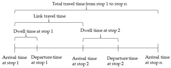
Figure 1.
Notation on bus travel time [28].
Travel time forecasts can be classified as short term/real-time forecasts and long-term forecasts. The difference between the two types is mainly due to their forecast horizons. The short-term travel time forecast aims to predict the travel time on the forecast horizon as equal to or less than a time value T [22], in which T could be defined case by case, e.g., 15 min. The long-term travel time forecast aims to predict the travel time as the longest forecast horizon of T, which could be the following day, week or year [29,30]. Long-term forecasting uses only historical average traffic condition data to predict future traffic status and travel time. Figure 2 illustrates the definition of travel time estimation and forecast/prediction.
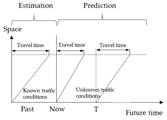
Figure 2.
Estimation and prediction notations on bus travel time [28].
Therefore, given the values of the travel time observed up to time T, the forecast/prediction at time T of the future realisation can be of two types:
- historical: the forecasting model obtained is applied to a future situation, for example, the following month or the following year, in the context of operational planning.
- real-time: current data, possibly combined with historical, are used to predict future values, for example, in the context of operations control.
Real-time forecasting can, in turn, follow the one-step-ahead forecasting approach, i.e., at time T + 1, realisations up to time T + 1 are used to forecast the value of the variable at time T + 2. In the event that the weights to be attributed to the previous creations decrease over time, there is the approach known in the literature as “exponential smoothing” [31].
In transit systems, travel time (TT) forecasts are used both for operations and monitoring planning [32,33,34,35,36,37], and different methods and models have been developed both for long- and short-term. Below, the literature is reviewed, and the pros and cons of each proposed approach are pointed out. Long-term travel times that are forecast for bus services [38,39,40] have been studied through regression methods and time series methods. Regression methods explain travel time (the dependent variable) through a set of independent variables (e.g., loads, street characteristics). To point out that nonlinear relationships between independent and dependent variables can exist [38], more complex models were developed, e.g., k-nearest neighbour regression, support vector regression, project pursuit regression, and artificial neural networks. Although such methods do not give satisfactory results when traffic conditions are not stable, they are largely applied [38,39,40] because they reveal which independent variables are relevant or most important for the reproduction/forecast of travel times.
Time-series-based methods focus on the relationship between the variables to be predicted (travel time) through the analysis of historical data [41,42,43,44]. Their strength consists of the high calculation speed due to the simple formulation of the analysis algorithm and the small number of operating variables of the service: only the travel times of the bus relative to the instant in time to which they were found. They allow the structure of travel time variability to be highlighted and the effects over time (e.g., hours of the day, day of the week, time of year), which are relevant in the links where the buses travel alongside other traffic components [5,45], to be revealed.
Deepening studies developed for short-term forecasting, these works can be classified into time-series [46,47], regression models [8,48], artificial neural networks (ANNs) [8,49,50,51,52], Kalman filter [52,53,54,55], and nonparametric regression models (NPRs) [47,56,57,58]. Time series models, such as autoregressive integrated moving average (ARIMA) models and exponential smoothing models, can forecast based on historical values. Large variations in historical data could lead to significant differences between observations and forecasts because time series models depend on the transferability of historical trends (patterns) to forecast trends [50]. Regression models are used to predict travel time through linkage with context-specific independent variables (e.g., traffic conditions, road link characteristics). Given that the explanatory variables must be statistically independent of each other and many of the variables relating to transport systems are highly correlated [52], ANN models have been developed. In fact, ANN models allow complex nonlinear relationships to be pointed out and can also generate better results than other models such as Kalman filter-based methods, smoothing models, historical profiles, and real-time profiles [51]. However, ANN models take longer computational time for the training process than other models.
3. Forecasting Methodology and Data Analysis
The collected data are related to two lines in the city of Rome (Italy; Lines A and B) and one line (Line C) in the city of Lviv (Ukraine). Table 1 reports the characteristics of the investigated bus service lines (Rome and Lviv). Figure 3 shows the observed travel times during working days (i.e., from Monday to Friday). The travel time for each bus line is analysed in two cases: to the city centre and from the city centre. According to the time of the day, we can observe a similarity in the shape of the data if travel is to or from the city centre: two peak hours present in the mornings and afternoon. Particularly, for the investigated bus lines, the variance is higher in the afternoon peak hour than in the morning (e.g., for Line A, direction to city centre: 229,800 sec2 vs. 160,284 sec2; direction from city centre: 155,034 sec2 vs. 110,413 sec2). Moreover, given that the roads are congested during peak hours and less congested during nonpeak hours, and, subsequently, travel time is longer in rush hours than in nonpeak hours, time series allow these patterns to be captured. In the following sections, time-series components of bus travel time data are studied.

Table 1.
The investigated bus lines.
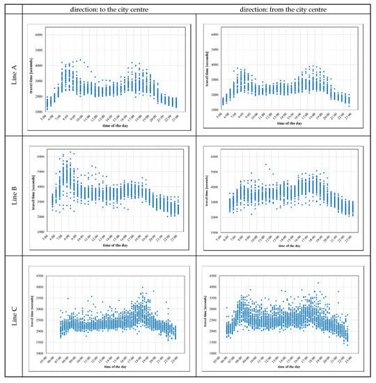
Figure 3.
Analysed bus lines: hourly fluctuation of travel time during working days.
4. Bus Travel Time Analysis and Forecasting
4.1. Bus Travel Time Analysis
Given a bus line, the bus travel time (TT) from a terminal to another is assumed to be the sum of the running time (RT) between successive stops and the dwelling time at stops (DW):
with RTi the running time between stop i and successive one i+1, and DWi the dwelling time spent at stop i.
Running time and dwelling time depends on a set of determinants. Running time is a function of speeds (related to flow composition and link flow), link characteristics (infrastructural and functional), context conditions (e.g., weather conditions; [59]), while dwelling time depends on on-board flow, alighting and boarding users, and bus features (e.g., number of doors, lift operations). Therefore, the analysis of bus travel time variability has to be investigated by capturing the fluctuations of these determinants. This pattern can be pointed out by time-series analysis.
A time series Yt can be composed of three components: a trend-cycle component Tt, a seasonal component St, and a remainder component Et that contains anything else in the time series. Therefore, assuming an additive relation among the three above components, the time series can be expressed as
Once the output of time series decomposition is used for forecasting, forecast accuracy has to be evaluated. An approach to evaluating the accuracy of forecasts relies on the application of the model on new data that were not used in the model calibration [31]. To do this, the available data are divided into two sets, training and test data. The training data is used to set up the forecasting model (i.e., identification of time-series components) and the test data is used to evaluate its accuracy (e.g., one week ahead). Since the test data is not used in determining the model, it should provide a reliable indication of how well the model is able to forecast by using new data. With this approach, the forecast error (ei) is assumed to be the difference between an observed value and its forecast, as follows:
where Yi denotes the ith observation and denotes a modelled value of Yi.
The most known accuracy measures [31] are MAE (mean absolute error), RMSE (root mean squared error), and MAPE (mean absolute percentage error). MAE and RMSE are scale-dependent measures and are based on absolute errors or squared errors :
On the other hand, MAPE has the advantage of being scale-independent:
with , which measures the percentage error.
4.2. Bus Travel Time Forecasting
As mentioned above, the used data refer to observed values of three bus lines during some working days of 10 consecutive weeks in Rome and Lviv. The last two weeks were set up as the test set, while the remaining weeks as the training set. Therefore, the time-series period was set in a week (five working days).
The time series decomposition (Figure 4 and Figure 5) was performed through seasonal and trend decomposition using the loess (STL; [60,61]) method implemented in R software [31]. The results analysis can be pointed out, and it shows similarities with patterns revealed in other urban contexts ([32,45,62]):
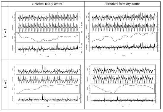
Figure 4.
Travel time STL decomposition with weekly period (8 weeks): Rome.
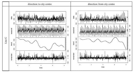
Figure 5.
Travel time STL decomposition with weekly period (8 weeks): Lviv.
- trends/cycles (T): small differences between maximum and minimum values, i.e., less than 5% for Line A, and about 2% for Lines B and C;
- weekly seasonality (S; Figure 6): the effects emerge for all days, with a periodic shape; differences emerge among the first and last days of the week (i.e., Monday/Tuesday vs. Thursday/Friday);
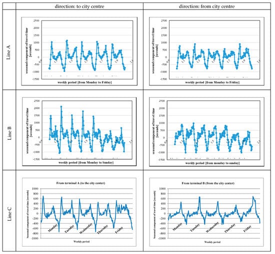 Figure 6. Seasonal components of the analysed bus lines.
 - daily seasonality (S; Figure 6):
- ○
- quite relevant for different hours of the day; as expected, it is influenced by the variance of traffic flows (i.e., buses share the lanes with other traffic components and bus travel time is influenced);
- ○
- quite different for routes to or from the city centre; higher values were revealed in the morning due to high concentrations of constrained trip arrivals (e.g., systemic trips, such as to work or school); on the other hand, the effects are more spread along the hours in the afternoon.
- remainder (E): low contributions in terms of variance of about 29% (Line A) and 21% (Line B) for Rome, while it is quite high in Lviv (Line C); it reflects the singular variability revealed in some days because of chance events concentrated in time and space rather than structural factors (Table 2).
 Table 2. Variance (σ2) and mean (µ) of the observed travel time (Y) and the remainder (E).
The capability to reproduce the observed data is then tested by using trend/cycle (Tt) and daily/hourly seasonality (St; i.e., time-series systematic components). The modelled error e can be assumed to be the remainder E (i.e., e ≡ E).
Figure 7 shows an example of a comparison between observed and modelled travel time for the test set, while Table 3 reports the accuracy for the investigated period. As synthetised by MAPE (smaller than 8%), the systemic component of travel time (i.e., trend/cycle and seasonality) allows the main part of variance to be explained. It means an average error in reproducing travel time less than 3 min (and about 1 min for Line B from the city centre) for the investigated lines. These accuracy metrics have the same magnitude as those we can find in the literature ([19,27,45,54]).
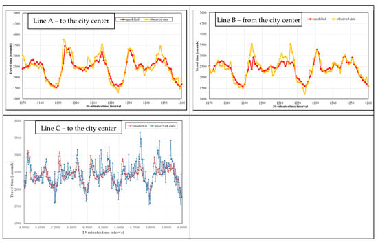
Figure 7.
Example of a comparison between observed and forecasted/modelled values.

Table 3.
Accuracy indicators of a route of Lines A, B and C.
The results of these analyses refer to the improvement of long-term travel time forecasting, but they can suggest new research opportunities for short-term forecasting, as also suggested by Cristobal et al. [8], who proposed short-term travel bus methods based on the similarity between historical ones.
4.3. Discussion
The comparison of the bus lines operating in two different (both in size and economic structure) cities pointed out a number of major findings. Bus lines in Lviv operate within the historical centre of the city, while in Rome, the study area merges suburbs with the inner-city area.
As regards spatial form, the inner area of Rome is surrounded by radially distributed roads. Lviv is an Eastern European city with a strong influence from Western cities in its urbanisation. Both the study areas are characterised by narrow streets and buses shares the lanes; therefore, their commercial speed is highly influenced by private traffic. In relation to bus travel time, there are no significant differences in patterns, with high values during morning and afternoon peak hours.
An in-depth comparison between Lviv and Rome showed that the travel time pattern is not strictly dependent on the size of the cities, but it is related to traffic jams (due mainly to lifestyle, e.g., starting of working day). Lviv presents a not-high perturbation during the morning, as indeed happens in Rome, where the high concentration of traffic dominates. Therefore, there is also a very similar pattern in relation to time distribution along the day, although Rome sees activity in the early morning and afternoon, and Lviv does not. The same is reflected in departures from the centre in the afternoon.
Finally, the differences between Rome and Lviv are primarily due to city morphology and lifestyle. The Rome study area has a road network with narrow streets, and it favours an increase of time during the morning peak hour due to high demand, with a high concentration of trip arrivals on time at the workplace or school. The buses share the lanes and necessarily require travel time to be longer. The second reason is lifestyle and the start of work time, in particular of offices and the opening time of shops and stores. While Rome has two main peak hours and more specific regulations (in Rome, a limited traffic zone has been implemented), in Lviv, the circulation of traffic is always allowed in the morning.
According to these first results, the proposed forecasting methods present high performance in covering variances. Of course, the transferability of results in terms of accuracy issues is not direct, and city-specific surveys are needed. Additionally, the general conclusion is that a more systemic approach could be used in forecasting travel time by trying to define more comprehensive methods that are able to capture the characteristics of traffic, taking into account that some features are city-specific. Results, such as those derived in this paper, can contribute to more effective and rational management of resources, offering to mobility agency technicians an easy-to-apply method for designing or revising timetables and scheduled services.
Further analyses are also in progress to improve these first results by developing other analyses through the inclusion of zonal and level-of-service attributes (e.g., traffic volumes, passive and active accessibility) and the characteristics of users that reach these areas for daily activity, as well as alighting and boarding flows. Currently, the travel time variable has been the only independent variable taken into consideration. It does not capture the influence of factors such as weather conditions, road pavement conditions, and pedestrian flows. A time series-based regression model that also includes more independent variables that capture the above effects is under development. Finally, the degree of transferability of the models and the obtainable accuracy is a work in progress.
5. Conclusions
An investigation of bus travel time variability was carried out, and the first results for developing an easy-to-apply methodology for the urban areas of Rome and Lviv are presented. The findings can be used by urban mobility agency technicians for designing transit service timetables and vehicle scheduling in the replanning of existing lines. The developed approach focuses on the systematic components of travel time. The results are mainly devoted to bus lines that share the road lanes with other traffic components (e.g., cars, freight vehicles, and so on). The analyses were performed through time-series methods, which allowed factors such as trends, seasonal variations, cycles, and irregular components to be pointed out. Time of the day as well as the day of the week (i.e., Wednesday vs. Thursday) were discovered to have significant effects on travel time variability, and, if rightly modelled, performing forecasts can be obtained. Moreover, the findings can be integrated into a short-term approach, which, traditionally, is not considered. In fact, the development of models for short-term travel time forecasts that consider the variety of different factors, such as demand, transport conditions, and weather conditions, is a research challenge. From the above statements, the further development of this study germinates the availability of further data on bus line operations and loads, data on other vehicles with whom lanes are shared (e.g., floating car data for revealing local traffic patterns), in-depth analysis of residuals coming from time-series decomposition, as well as an approach to incorporate covariates such as weather data to model travel time as this factor might impact bus line travel time significantly. Finally, bus travel time forecasts are based on profile similarities through the time-series and regression methods.
Author Contributions
Conceptualization, A.C.; methodology, A.C.; software, A.P.; validation, A.C. and A.P.; formal analysis, A.C. and A.P.; investigation, A.C. and A.P.; data curation, A.C. and A.P.; writing—original draft preparation, A.C. and A.P.; writing—review and editing, A.C.; visualization, A.C. and A.P.; supervision, A.C. All authors have read and agreed to the published version of the manuscript.
Funding
This research received no external funding. The APC was funded by MDPI.
Acknowledgments
The authors wish to thank M. Zhuk, V. Kovalyshyn and V. Hilevych, for having shared data from Lviv. The authors wish to thank the anonymous reviewers for their suggestions, which were most useful in revising the paper.
Conflicts of Interest
The authors declare no conflict of interest.
References
- Russo, F.; Comi, A. Investigating the effects of city logistics measures on the economy of the city. Sustainability 2020, 12, 1439. [Google Scholar] [CrossRef]
- Musolino, G.; Polimeni, A.; Vitetta, A. Freight vehicle routing with reliable link travel times: A method based on network fundamental diagram. Transp. Lett. 2018, 10, 159–171. [Google Scholar] [CrossRef]
- Birr, K.; Jamroz, K.; Kustra, W. Travel time of public transport vehicles estimation. Transp. Res. Procedia 2014, 3, 359–365. [Google Scholar] [CrossRef][Green Version]
- Fusco, G.; Colombaroni, C.; Isaenko, N. Short-term speed predictions exploiting big data on large urban road networks. Transp. Res. Part C Emerg. Technol. 2016, 73, 183–201. [Google Scholar] [CrossRef]
- Comi, A.; Nuzzolo, A.; Brinchi, S.; Verghini, R. Bus travel time variability: Some experimental evidences. Transp. Res. Procedia 2017, 27, 101–108. [Google Scholar] [CrossRef]
- Karami, Z.; Kashef, R. Smart transportation planning: Data, models, and algorithms. Transp. Eng. 2020, 2, 100013. [Google Scholar] [CrossRef]
- Cats, O. Determinants of bus riding time deviations: Relationship between driving patterns and transit performance. J. Transp. Eng. Part A Syst. 2019, 145, 04018078. [Google Scholar] [CrossRef]
- Cristóbal, T.; Padrón, G.; Quesada-Arencibia, A.; Alayón, F.; De Blasio, G.; Garcia, C.D. Bus travel time prediction model based on profile similarity. Sensors 2019, 19, 2869. [Google Scholar] [CrossRef]
- Wu, J.; Wu, Q.; Shen, J.; Cai, C. Towards attention-based convolutional long short-term memory for travel time prediction of bus journeys. Sensors 2020, 20, 3354. [Google Scholar] [CrossRef]
- Balasubramanian, P.; Rao, K. An adaptive long-term bus arrival time prediction model with cyclic variations. J. Public Transp. 2015, 18, 6. [Google Scholar] [CrossRef]
- Jeong, R.H.; Rilett, L.R. Prediction model of bus arrival time for real-time applications. Transp. Res. Rec. 2005, 1927, 195–204. [Google Scholar] [CrossRef]
- Comi, A.; Nuzzolo, A.; Brinchi, S.; Verghini, R. Bus dispatching irregularity and travel time dispersion. In Proceedings of the 5th IEEE International Conference on Models and Technologies for Intelligent Transportation Systems (MT-ITS), Naples, Italy, 26 June 2017; pp. 856–860. [Google Scholar]
- Jeffery, D. Guidelines for Assessing the Transferability of an Innovative Urban Transport Concept; NICHES+, Coordination Action funded by the European Commission under the Seventh Framework Programme for R&D, Sustainable Surface Transport; 2011; Available online: www.rupprecht-consult.eu/uploads/tx_rupprecht/NICHES_Guideline_Transferability_01.pdf (accessed on 28 July 2020).
- Wu, F.; Hu, X.; An, S.; Zhang, D. Exploring passengers’ travel behaviors based on elaboration likelihood model under the impact of intelligent bus information. J. Adv. Transp. Vol. 2019, 9095279. [Google Scholar] [CrossRef]
- Rupprecht Consult. Guidelines for Developing and Implementing a Sustainable Urban Mobility Plan, Second Edition. 2019. Available online: https://www.eltis.org/mobility-plans/sump-guidelines (accessed on 20 July 2020).
- Mazloumi, E.; Rose, G.; Currie, G.; Sarvi, M. An integrated framework to predict bus travel time and its variability using traffic flow data. J. Intell. Transp. Syst. 2011, 15, 75–90. [Google Scholar] [CrossRef]
- Kimpel, T.J.; Strathman, J.G.; Callas, S. Improving scheduling through monitoring using AVL/APC data. In Proceedings of the 9th International Conference on Computer-Aided Scheduling of Public Transport (CASPT), San Diego, CA, USA, 9–11 August 2004. [Google Scholar]
- Turochy, R.; Smith, B. Measuring variability in traffic conditions by using archived traffic data. Transp. Res. Rec. 2002, 1804, 168–172. [Google Scholar] [CrossRef]
- Ceder, A. Public Transit Planning and Operation: Modeling, Practice and Behavior, 2nd ed.; CRC Press: Boca Raton, FL, USA; Taylor & Francis Group: Abingdon, UK, 2015. [Google Scholar]
- Bates, J.; Polak, J.; Jones, P.; Cook, A. The valuation of reliability for personal travel. Transp. Res. Part E 2001, 37, 191–229. [Google Scholar] [CrossRef]
- Lam, T.C.; Small, K.A. The value of time and reliability: Measurement from a value pricing experiment. Transp. Res. Part E 2001, 37, 231–251. [Google Scholar] [CrossRef]
- Nuzzolo, A.; Comi, A. A subjective optimal strategy for transit simulation models. J. Adv. Transp. 2018, 2018, 8797328. [Google Scholar] [CrossRef]
- Sun, C.; Arr, G.; Ramachandran, R.P. Vehicle reidentification as method for deriving travel time and travel time distributions. Transp. Res. Rec. 2003, 1826, 25–31. [Google Scholar] [CrossRef]
- Sun, D.; Luo, H.; Fu, L.; Liu, W.; Liao, X.; Zhao, M. Predicting bus arrival time on the basis of global positioning system data. Transp. Res. Rec. 2007, 2034, 62–72. [Google Scholar] [CrossRef]
- Comi, A.; Zhuk, M.; Kovalyshyn, V.; Hilevych, V. Investigating bus travel time and predictive models: A time series-based approach. Transp. Res. Procedia 2020, 45, 692–699. [Google Scholar] [CrossRef]
- Nuzzolo, A.; Comi, A. Advanced public transport and intelligent transport systems: New modelling challenges. Transp. A Transp. Sci. 2016, 12, 674–699. [Google Scholar] [CrossRef]
- Gong, X.; Guo, X.; Dou, X.; Lu, L. Bus travel time deviation analysis using automatic vehicle location data and structural equation modeling. J. Adv. Transp. Vol. 2015. [Google Scholar] [CrossRef][Green Version]
- Kieu, L.M.; Bhaskar, A.; Chung, E. Benefits and issues for bus travel time estimation and prediction. In Proceedings of the Australasian Transport Research Forum 2012, Perth, Australia, 26–28 September 2012. [Google Scholar]
- Liu, H. Travel Time Prediction for Urban Networks. Ph.D. Thesis, Netherlands Research School for Transport, Infrastructure and Logistics, TU Delft, The Netherlands, 2008. [Google Scholar]
- van Lint, J.W.C.; Hoogendoorn, S.P.; van Zuylen, H.J. Accurate freeway travel time prediction with state-space neural networks under missing data. Transp. Res. Part C Emerg. Technol. 2005, 13, 347–369. [Google Scholar] [CrossRef]
- Hyndman, R.J.; Athanasopoulos, G. Forecasting: Principles and Practice, 2nd ed.; OTexts: Melbourne, Australia, 2018; Available online: OTexts.com/fpp2 (accessed on 17 July 2020).
- Rajbhandari, R. Bus Arrival Time Prediction Using Stochastic Time Series and Markov Chains. Ph.D. Thesis, Faculty of New Jersey Institute of Technology, Newark, NJ, USA, 2006. [Google Scholar]
- Bolshinsky, E.; Freidman, R. Traffic Flow Forecast Survey; Technical Report; Technion–Israel Institute of Technology: Haifa, Israel, 2012. [Google Scholar]
- Fan, W.; Gurmu, Z. Dynamic travel time prediction models for buses using only GPS data. Int. J. Transp. Sci. Technol. 2015, 4, 353–366. [Google Scholar] [CrossRef]
- Moreira-Matias, L.; Mendes-Moreira, J.; de Sousa, J.F.; Gama, J. Improving mass transit operations by using AVL-based systems: A survey. IEEE Trans. Intell. Transp. Syst. 2015, 16, 1636–1653. [Google Scholar] [CrossRef]
- Yu, Z.; Wood, J.S.; Gayah, V.V. Using survival models to estimate bus travel times and associated uncertainties. Transp. Res. Part C Emerg. Technol. 2017, 74, 366–382. [Google Scholar] [CrossRef]
- He, P.; Jiang, G.; Lam, S.K.; Tang, D. Travel-time prediction of bus journey with multiple bus trips. IEEE Trans. Intell. Transp. Syst. 2019, 20, 4192–4205. [Google Scholar] [CrossRef]
- Chen, M.; Liu, X.; Xia, J.; Chien, S.I. A dynamic bus-arrival time prediction model based on APC data. Comput. Aided Civ. Infrastruct. Eng. 2004, 19, 364–376. [Google Scholar] [CrossRef]
- Mendes-Moreira, J.; Jorge, A.M.; de Sousa, J.F.; Soares, C. Comparing state-of-the-art regression methods for long term travel time prediction. Intell. Data Anal. 2012, 16, 427–449. [Google Scholar] [CrossRef]
- Moreira-Matias, L.; Cats, O.; Gama, J.; Mendes-Moreira, J.; de Sousa, J.F. An online learning approach to eliminate bus bunching in real-time. Appl. Soft Comput. 2016, 47, 460–482. [Google Scholar] [CrossRef]
- Williams, B.M.; Hoel, L.A. Modeling and forecasting vehicular traffic flow as a seasonal ARIMA process: Theoretical basis and empirical results. J. Transp. Eng. 2013, 129, 664–672. [Google Scholar] [CrossRef]
- Jeong, R.H. The Prediction of Bus Arrival Time Using Automatic Vehicle Location Systems Data. Ph.D. Thesis, Texas A&M University, College Station, TX, USA, 2004. [Google Scholar]
- Billings, D.; Yang, J.-S. Application of the ARIMA models to urban roadway travel time prediction—A case study. In Proceedings of the 2006 IEEE International Conference on Systems, Man and Cybernetics, Taipei, Taiwan, 8 October 2006; Volume 3, pp. 2529–2534. [Google Scholar]
- Suwardo, M.N.; Ibrahim, K. ARIMA models for bus travel time prediction. J. Inst. Eng. 2010, 71, 49–58. [Google Scholar]
- Yetiskul, E.; Senbil, M. Public bus transit travel-time variability in Ankara (Turkey). Transp. Policy 2012, 23, 50–59. [Google Scholar] [CrossRef]
- Ahmed, M.; Cook, A. Analysis of freeway traffic time series data by using Box–Jenkins techniques. Transp. Res. Board 1979, 722, 1–9. [Google Scholar]
- Smith, B.L.; Williams, B.M.; Oswald, R.K. Comparison of parametric and nonparametric models for traffic flow forecasting. Transp. Res. Part C 2002, 10, 303–321. [Google Scholar] [CrossRef]
- Lin, W.H.; Zeng, J. Experimental study of real-time bus arrival time prediction with GPS data. Transp. Res. Rec. 1999, 1666, 101–109. [Google Scholar] [CrossRef]
- Kalaputapu, R.; Demetsky, M.J. Modeling schedule deviations of buses using automatic vehicle-location data and artificial neural networks. Transp. Res. Rec. 1995, 1479, 44–52. [Google Scholar]
- Smith, B.L.; Demetsky, M.J. Short-term flow prediction: Neural network approach. Transp. Res. Rec. 1995, 1453, 98–104. [Google Scholar]
- Park, D.; Rilett, L.R. Forecasting freeway link travel times with a multilayer feedforward neural network. Comput. Aided Civ. Infrastruct. Eng. 1999, 14, 357–367. [Google Scholar] [CrossRef]
- Chien, S.; Ding, Y.; Wei, C. Dynamic bus arrival time prediction with artificial neural network. ASCE J. Transp. Eng. 2002, 128, 429–438. [Google Scholar] [CrossRef]
- Chen, M.; Chien, S. Dynamic freeway travel-time prediction with probe vehicle data: Link based versus path based. Transp. Res. Rec. 2001, 1879, 89–98. [Google Scholar] [CrossRef]
- Cathey, F.; Dailey, D. A prescription for transit arrival/departure prediction using AVL data. Transp. Res. Part C 2003, 11, 241–264. [Google Scholar] [CrossRef]
- Shalaby, A.; Farhan, A. Prediction model of bus arrival and departure times using AVL and APC data. J. Public Transp. 2004, 7, 41–61. [Google Scholar] [CrossRef]
- Davis, G.; Nihan, N. Nonparametric regression and short-term freeway traffic forecasting. J. Transp. Eng. 1991, 117, 178–188. [Google Scholar] [CrossRef]
- Sun, H.; Liu, H.X.; Xiao, H.; He, R.R.; Ran, B. Use of local linear regression model for short-term traffic forecasting. Transp. Res. Rec. 2003, 1936, 143–150. [Google Scholar] [CrossRef]
- Qi, Y.; Smith, B.L. Identifying nearest-neighbors in a large-scale incident data archive. Transp. Res. Rec. 2004, 1879, 89–98. [Google Scholar] [CrossRef]
- Zhang, X.; Chen, M. Quantifying the impact of weather events on travel time and reliability. J. Adv. Transp. Vol. 2019. [Google Scholar] [CrossRef]
- Cleveland, R.B.; Cleveland, W.S.; Terpenning, I. STL: A seasonal-trend decomposition procedure based on loess. J. Off. Stat. 1990, 6, 3. [Google Scholar]
- Jeon, S.; Hong, B. Monte Carlo simulation-based traffic speed forecasting using historical big data. Future Gener. Comput. Syst. 2016, 65, 182–195. [Google Scholar] [CrossRef]
- Bai, C.; Peng, Z.R.; Lu, Q.C.; Sun, J. Dynamic bus travel time prediction models on road with multiple bus routes. J. Adv. Transp. Vol. 2015. [Google Scholar] [CrossRef]
© 2020 by the authors. Licensee MDPI, Basel, Switzerland. This article is an open access article distributed under the terms and conditions of the Creative Commons Attribution (CC BY) license (http://creativecommons.org/licenses/by/4.0/).