Article

Machine Learning-Based Error Modeling to Improve GPM IMERG Precipitation Product over the Brahmaputra River Basin

by
Md Abul Ehsan Bhuiyan
1,*,
Feifei Yang
2,
Nishan Kumar Biswas
3,
Saiful Haque Rahat
4 and
Tahneen Jahan Neelam
5
1
Department of Natural Resources and the Environment, University of Connecticut, Storrs, CT 06269-3088, USA
2
Department of Civil and Environmental Engineering, University of Connecticut, Storrs, CT 06269-3088, USA
3
Department of Civil and Environmental Engineering, University of Washington, Seattle, WA 98195, USA
4
Department of Chemical and Environmental Engineering, University of Cincinnati, Cincinnati, OH 45220, USA
5
Department of Biological and Environmental Engineering, Cornell University, Ithaca, NY 14853, USA
*
Author to whom correspondence should be addressed.
Forecasting 2020, 2(3), 248-266; https://doi.org/10.3390/forecast2030014
Submission received: 10 June 2020 / Revised: 20 July 2020 / Accepted: 21 July 2020 / Published: 25 July 2020
(This article belongs to the Special Issue Advances in Hydrological Forecasting)

Abstract

:
The Integrated Multisatellite Retrievals for Global Precipitation Measurement (GPM) (IMERG) Level 3 estimates rainfall from passive microwave sensors onboard satellites that are associated with several uncertainty sources such as sensor calibration, retrieval errors, and orographic effects. This study aims to provide a comprehensive investigation of multiple machine learning (ML) techniques (Random Forest, and Neural Networks), to stochastically generate an error-corrected improved IMERG precipitation product at a daily time scale and 0.1°-degree spatial resolution over the Brahmaputra river basin. In this study, we used the operational IMERG-Late Run version 06 product along with several meteorological and land surface parameters (elevation, soil type, land type, soil moisture, and daily maximum and minimum temperature) to produce an improved precipitation product in the Brahmaputra basin. We trained, tested, and optimized ML algorithms using 4 years (from 2015 through 2019) of reference rainfall data derived from the rain gauge. The ML generated precipitation product exhibited improved systematic and random error statistics for the study area, which is a strong indication for using the proposed algorithms in retrieving precipitation across the globe. We conclude that the proposed ML-based ensemble framework has the potential to quantify and correct the error sources for improving and promoting the use of satellite-based precipitation estimates for water resources applications.

1. Introduction

The accurate estimation of precipitation incorporates a significant impact on the hydrology, vegetation, natural life, and ecology of any water resource system [1,2]. Despite the fact that precipitation is one of the most imperative parameters for water resource management, documenting precise precipitation information on a global scale is a challenge for climate experts and the scientific community [3,4,5]. While in situ rain gauge station and weather radar data are the most common sources to obtain precipitation information, satellite-based precipitation products have been recognized as a subordinate source of precipitation data to overcome the restrictions due to inadequate spatial coverage or uneven conveyance from ground-based observations [1,6,7,8,9]. However, complex terrain regions with high-altitude satellite precipitation estimates are associated with substantial error due to variability and uncertainty introduced by orographic effects [10,11,12,13,14,15,16].
Different satellite-based precipitation products are accessible to supply precipitation at fine spatio-temporal resolutions for a broad range of applications [15,16]. Among these precipitation products, the Integrated Multi-satellite Retrievals for GPM (IMERG) is a combination of features of three multi-satellite precipitation products including (1) Tropical Rainfall Measurement Mission (TRMM) Multi-satellite Precipitation Analysis (TMPA), (2) Climate Prediction Center Morphing (CMORPH) and (3) Precipitation Estimation from Remotely Sensed Information using Artificial Neural Networks (PERSIANN) deemed to have advantages over available satellite-based precipitation products [1,3,17,18]. While IMERG and ground-based observations agree reasonably well for the variations of mean daily precipitation, IMERG tends to overestimate higher monthly precipitation amounts and underestimate dry season precipitation amounts, specifically in multiple regions of Asia [3,19,20].
Moreover, previous studies have assessed the performance of IMERG over varied topographic and geographic features considering seasonal characteristics [19,21,22,23,24,25,26,27,28,29]. The validation of the IMERG dataset using ground-based observations (i.e., gauges and radar) in conterminous US and Canada suggests an overall improvement in surface precipitation measurement from previous similar products [22,26]. Relative to Tropical Rainfall Measurement Mission (TRMM), IMERG displays improvement associated with the misrepresentation of the rainfall pattern with significant bias reduction in the US conterminous [22] and provides a better correlation in daily and monthly scale in mainland China [27,29,30]. In addition, IMERG showed poor performance even with its improved ability to sense frozen precipitation and deemed to be unreliable over Northern China [31]. Similarly, Murali et al. [24] showed region-specific biases and underestimation for the IMERG products compared to the observed precipitation over the Indian subcontinent. Islam et al. [32] concluded that the performance of IMERG is relatively unsatisfactory for the winter season in Bangladesh and deemed it to be inefficient to estimate the amount of rainfall in general. Such inconsistencies in IMERG products might be associated with various sources of errors causing a detrimental impact on the hydrologic investigation [15,16,33,34], and the need to eliminate these errors for certain regions like Ganges Brahmaputra Meghna (GBM) basin is paramount.
Historically, a significant divergence of opinion on the development of the Brahmaputra river basin has existed among the three demographic giants (namely China, India, and Bangladesh) in this region [35,36,37]. All these bordering countries are under ever-increasing pressure due to global change, severe water scarcity, and rising demands from population growth [35,38]. Owing to the geopolitical relationships among the countries, Ray et al. [39] identify the absence of an authoritative, dependable, and comprehensive network of basin-wide information on climate as a critical compounding factor in the Brahmaputra basin. A better representative, error-corrected satellite precipitation dataset is essential to fill in the current knowledge gaps in this region.
Therefore, error modeling is vital for improving the use of satellite-based precipitation product (GPM IMERG Precipitation estimates) in precipitation-sensitive applications such as hydrological modeling [40]. The first step to error modeling is to recognize the physical error factors and then evaluate the related error magnitudes. Research on error analysis of the satellite precipitation product has been reported in several past studies, which considered the dependence on precipitation rates and types, as well as surface conditions like soil moisture and land cover [40,41]. A multidimensional satellite rainfall error model (SREM2D) developed by Hossain and Anagnostou [42] has been used in several error modeling studies of satellite rainfall products [43,44,45]. Bhuiyan et al. [33] recently applied machine learning-based error modeling to evaluate the errors of passive microwave precipitation retrievals based on high-resolution ground radar-rainfall estimates. In that study, they combined meteorological and land surface data from multiple sources to study the impact of land surface conditions (e.g., vegetation cover and soil moisture) on the passive microwave retrieval error.
Recently, nonparametric models have become increasingly popular in weather forecasting, climate change prediction, and the modeling of hydrological processes [14,15,16,46,47,48,49,50]. Moreover, Non-parametric machine learning techniques such as Quantile Regression Forests (QRF) [51], Random Forests (RF) [52], Classification and Regression Trees (CART) [53], Bayesian Additive Regression Trees (BART) [54], and Neural Networks (NN) [55,56,57] have become especially popular in hydro-meteorological application [14,33,58,59,60,61,62]. Specifically, NN and RF have been used in several studies to predict precipitation and showed promising results in quantifying precipitation uncertainties for global hydrologic applications [63,64,65,66,67].
The objective of this study is to investigate the use of two machine learning-based error models: Neural Network (NN) and Random forest (RF) in representing the realizations of error-adjusted IMERG rainfall products. The prediction consistency and dependence of NN and RF models in terms of point estimation of GPM IMERG retrieval error are explored carefully to show how the two models perform under different evaluation criteria. The paper is structured as follows: in Section 2, we describe the study area and dataset. Section 3 describes the prediction model, validation methodology, and the performance evaluation error metrics. Evaluation results and discussions are explored in Section 4. Conclusions and recommendations are discussed in Section 5.

2. Study Area and Datasets

2.1. Study Area

The GBM basin consists of the Ganges, Brahmaputra, and Meghna rivers originating from the Himalayas and Vindhya ranges flowing through China, Bhutan, Nepal, India, and Bangladesh and ultimately connecting with the inlet at the Bay of Bengal [68]. In terms of hydrologic vulnerability assessment, GBM deserves special attention for some reasons. For instance, the GBM basin dominates annual flooding cycles, the region of inundation, and the withdrawal of floodwaters based on the hydrologic settings of the adjacent countries surrounded by it [46,69].
Moreover, under changing climate scenarios, dry season rainfall pattern is projected to further decrease for elevated temperature while monsoon rainfall is expected to be more intense resulting from the glacier or early snowmelt. Therefore, a basin level assessment with a more comprehensive evaluation of climate change impacts is mandatory for flood regions such as Nepal, India and Bangladesh [70,71,72]. Improved IMERG data with limited error might have the utility for the large-scale water resources modeling in GBM to assess climate impact [21,29,39].
Inside the GBM basin, the Brahmaputra River (alternatively known as Yarlung Tsangpo river in China) Basin in Southeast Asia is the fourth largest fluvial system in the world [73]. This basin has a drainage area of about 570,000 km2 with rugged terrain, accommodating a population of 130 million which is spread over China, India, Bhutan, and Bangladesh [74]. Hydrological modeling for this region is crucial and complex due to its intense seasonal rainfall, unevenly distributed and poorly maintained real-time rain gauge data, and convoluted transboundary issues [75,76].
The study area has a varied topographic gradient from around 8500 m MSL at the origin to about 2 m MSL at the outlet where it meets the Ganges. The upper Brahmaputra river basin lies in the temperate climate zone with mostly unpopulated area whereas the lower Brahmaputra river basin is in a tropical climate that is densely populated and vulnerable to monsoon flooding [77,78]. Hence, this region has a higher number of in situ stations. The study area and the corresponding in situ gauge networks consisting of 120 stations are shown in Figure 1.

2.2. Datasets

The datasets used in this study span from March 2015 to March 2019. The daily accumulated precipitation datasets from these stations were collected from the Central Water Commission, India; Bangladesh Meteorological Department, Bangladesh, and the Department of Hydrometeorology, Nepal. The gauge measurement were averaged at 0.1 × 0.1 degree grid resolution. For this study, we used the operational IMERG-Late Run version 06 product [79] which was the latest available late run product (https://disc.gsfc.nasa.gov/datasets/GPM_3IMERGDL_06/summary). IMERG precipitation has three different versions, (a) early run; (b) late run and (c) final run. In this study we used late run product which uses a climatological adjustment that incorporates gauge data. The IMERG late run product has both backward and forward morphing and retrieved from different passive microwave (PMW) and infrared (IR) sensors. We used the latest available product (V06) late run version of IMERG because the objective of this study was to focus on the operational use of this precipitation in short-term decision making, cropping, drought management, and water resources planning for the resource-limited stakeholder organizations. Moreover, the latest version of IMERG (V6) has a number of advantages over previous versions such as upgraded GPROF-TMI V05 incorporation into the dataset (https://gpm.nasa.gov/sites/default/files/document_files/IMERG_V06_release_notes_190503.pdf). IMERG (V6) is a high-resolution product available with 0.1 × 0.1 degree spatial and 30 min temporal resolution [6,79]. The dataset’s spatial coverage is from 90° N–90° S and temporal coverage is from April 2014 to the present (https://gpm.nasa.gov/data-access/downloads/gpm).
For model forcing, elevation data were extracted from a 30 × 30 DEM (Shuttle Radar Topography Mission) 1 Arc-Second Global (Digital Object Identifier (DOI) number:/10.5066/F7PR7TFT). Soil Moisture Active Passive (SMAP) Level-4 soil moisture data were collected from the National Snow and Ice Data Center for spatial coverage: N: 85.044, S: −85.044, E: 180, W: −180. This dataset has a 9 km Equal-Area Scalable Earth (EASE)-Grid spatial and 3-hourly temporal resolution [80]. The SMAP soil moisture data from March 2015 to March 2019 was used in this study. Daily maximum and minimum land surface temperature was collected from NASA Land Processes Distributed Active Archive Center (LP DAAC). The MOD11C1 version 06 products provide land surface temperature value in a 0.05° by 0.05° Climate Modeling Grid on a daily temporal scale with a latency of approximately 1 day [81]. For land type, USGS Global Land Cover Characterization (GLCC) product with 1 km spatial resolution was used [82]. Soil type was extracted from the FAO Harmonized World Soil Database [83]. Table 1 summarizes land surface and meteorological datasets.
All the meteorological datasets were resampled to 0.1° by 0.1° using the cubic spline method. The original soil moisture dataset was of 9 km EASE grid with 3 hourly temporal resolution. These datasets were averaged into the daily scale and resampled to 0.1° by 0.1° using the cubic spline method. Daily maximum and minimum temperature data were 0.05° by 0.05°. These data were resampled to the same resolution of the principal forcing data (precipitation) using the cubic spline method. Regarding land surface variables, Shuttle Radar Topographic Mission (SRTM) based Digital Elevation Model (DEM) elevation was extracted for each of the grid locations of the precipitation. Similarly, USGS land cover type and FAO soil type were extracted in each of the grid locations of precipitation. The in-situ precipitation was station-based (in discrete locations). For each day of the study period, all the available in-situ rainfall data were converted into gridded rainfall using Inverse Distance Weightage (IDW) method as mentioned in [84]. Finally, all daily data were mapped to the 0.1° grid chosen to be the final spatial grid for the error model to generate the error-corrected IMERG product. For the error models, the response variable is the rainfall estimate from rain gauge.

3. Methodology

3.1. Precipitation Error Modeling

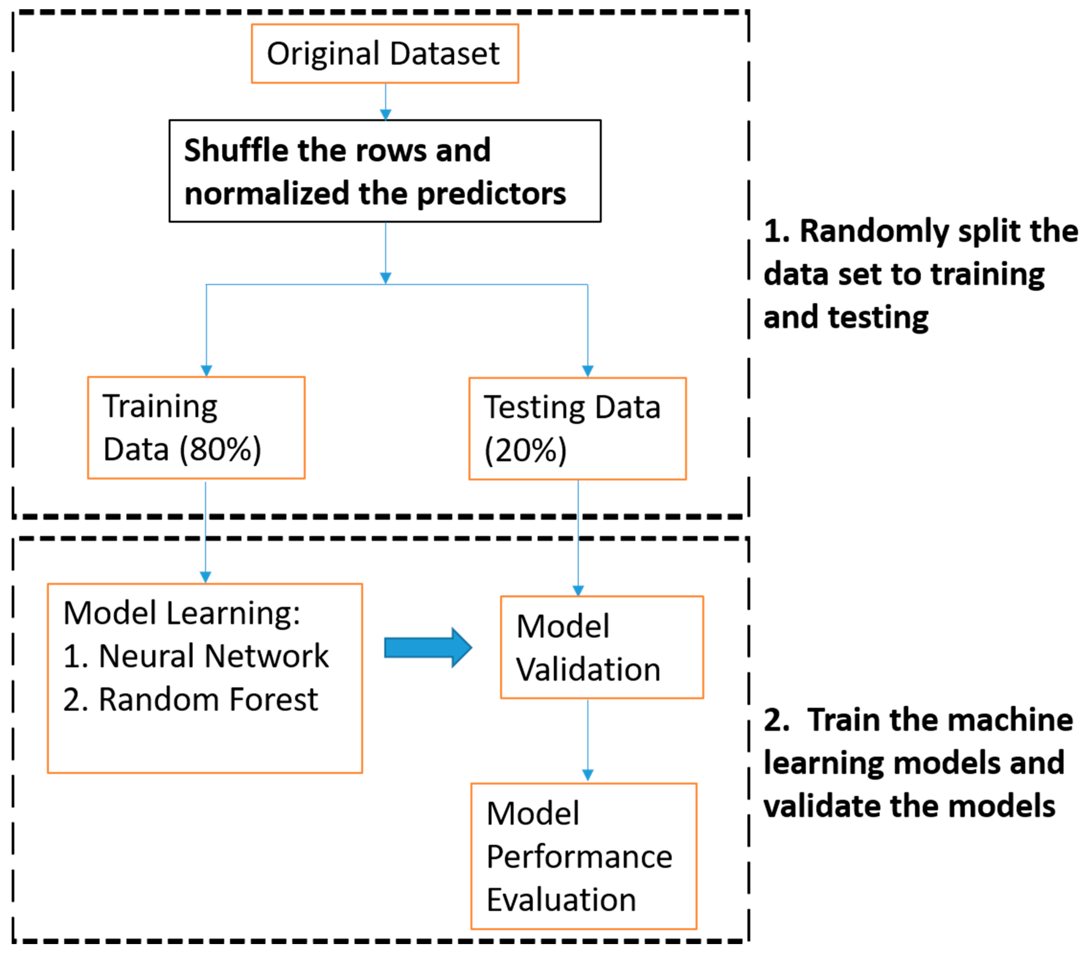
To develop the error models for the study area we used two machine learning techniques: Random Forests (RF) and Neural Network (NN), to improve GPM IMERG precipitation product. A schematic diagram of the error modeling process is shown in Figure 2. This study devised a randomized and out-of-sample validation experiment to quantify the uncertainty of IMERG precipitation product. Specifically, the two error models, (Neural Network and Random Forest) were developed on the training dataset and were used to predict the holdout dataset, which was applied for testing.
We used “sample” function in R programming to shuffle the row indices of all the dataset to reorder the rows of the dataset randomly. Then, we split 80% of the dataset into the training set and remaining 20% of them into the testing set. Specifically, randomly divided 121,046 rows of data were treated as training and 30,259 rows of the data as testing. To avoid overfitting, we used these independent test data to check the method’s accuracy on training data after training which adjusted network structure as well as optimization algorithm parameters of network weight. By using these data and according to the magnitude of mean squared residuals, the network parameters were adjusted. The performance of the error models was evaluated by comparing the error metrics described in Section 3.2.

3.1.1. Random Forests (RF)

To develop the precipitation error model, we used non-parametric Random Forest (RF) algorithm which uses ensembles (“forests”) of classification or regression trees [52]. Each tree depends on the values of a random vector sampled independently and with the same distribution for all trees in the forest. The generalization error for forests converges as the number of trees in the forest becomes large [85,86]. We used R package of “randomForest” and number of trees 1000 for the RF model, and the error for the model was converged before number of trees 1000 as shown in Figure 3.
Initially, to optimize the model, datasets were randomly divided into a training dataset, validation dataset, and test dataset based on the 8:1:1 split rule and the parameters were adjusted for this algorithm. One of the challenges in a data-driven machine learning algorithm is overfitting. In the RF algorithm, each tree chooses and permutes random subsets of input variables at each splitting node, which reduces overfitting and improves the strength of predictions [52]. Therefore, RF utilizes the optimal number “mtry” (size of the random subset of input variables) for split point selection at each node, which introduces randomness in the forests to reduce the correlation between trees [14]. After finalizing the model, we split 80% of the dataset into the training set and remaining 20% of them into the testing set. A schematic diagram is presented in Figure 4. The model testing results are described in Section 4.2.

3.1.2. Neural Network (NN)

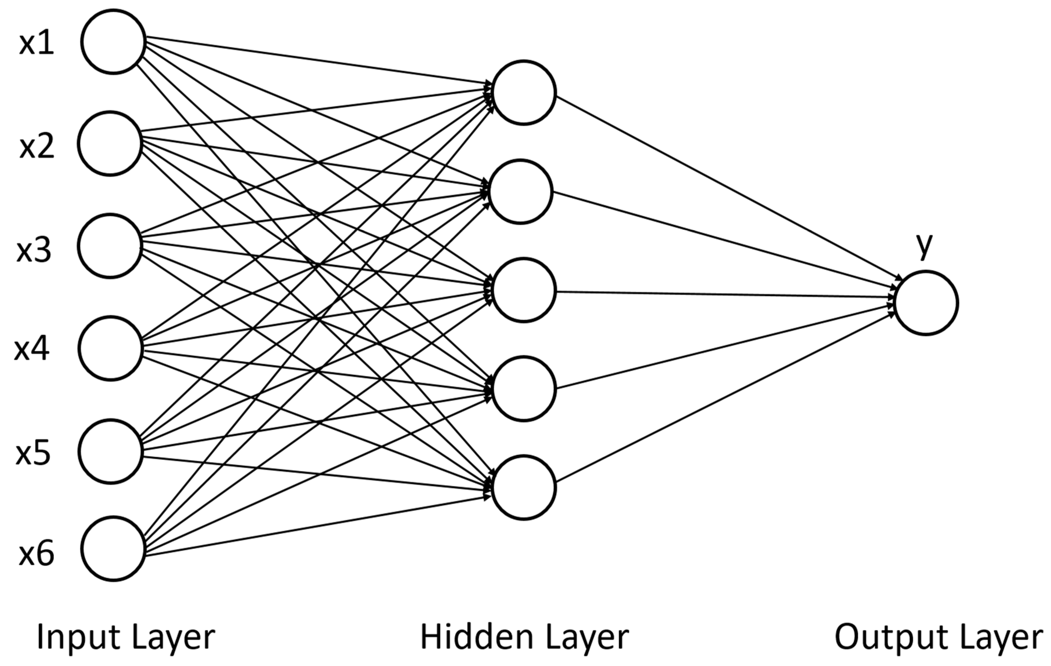
The neural network replicates the function of clusters of biological neurons that constitute an animal brain. The fundamental building blocks are called nodes and are used as information processing elements [55,56,57]. Through a training process, neural networks learn algorithms that can be fitted to the information for detailed data analysis. A schematic representation of Neural Network (NN) is shown in Figure 5. Such learning algorithms are defined by the utilization of a given output that is comparable to the predicted output and by adjusting the parameters as per the comparison.
These predicted outputs are usually transformed through the hidden layers of the neural network from the input data by weights in the parameter [87,88]. When an input enters the node, it gets multiplied by a weight value and the resulting value is either observer or passed to the next layer of the network, which can be helpful to understand the mechanism of such a concept. Suppose a neural network calculates an output y = f(x), for a given input x and weight, w. However, the training process is not completed yet. As such, the predicted output y will be different from the observed output x. To identify such discrepancies, error function E, like the sum of squared errors, SSE = i = 1 n ( y i x i ) 2 can be used; where y i is the ith value of the variable to be predicted. All weights keep getting adapted based on the rule of the learning algorithm.
The process stops when all the partial derivative,   d E d w of the error function with respect to the weights are smaller than the defined threshold. Such a methodology was implemented in order to reduce errors for satellite weather data propagation [89]. In this study, NN used backpropagation, namely the resilient backpropagation (RPROP) algorithm [90] which allowed for flexible settings through custom-choice of error and activation function. Finally, to optimize the error model, the calculation of generalized weights [91] was implemented and generated error corrected IMERG prediction. Table 2 summarizes the tuned hyperparameters for the algorithms used in this study.

3.2. Performance Evaluation Error Metrics

We tasked various error metrics to assess the error model performances. We evaluated the random error component based on the normalized centered root mean square error (NCRMSE), and defined as:
N C R M S E = 1 n i = 1 n [ y ^ i y i 1 n i = 1 n ( y ^ i y i ) ] 2 1 n i = 1 n y i
Here, y i is the reference rainfall, y ^ i is model predicted rainfall, and n is the quantity of samples used in the calculation. NCRMSE ranges from 0 (an optimal value) to positive infinity.
To measure the systematic error, we used mean relative error (MRE) which is the mean of the relative percentage error, calculated by the normalized average:
M R E = 1 n i = 1 n ( y ^ i y i y i )
MRE represents the magnitude and direction of error with positive value referring to overestimation while negative value referring to underestimation.
We applied Theil’s ‘coefficient of inequality’ for the model performances. Theil’s inequality coefficient U1 and U2 are expressed as below [92]:
U 1 = 1 n t = 1 n ( y t f t ) 2 1 n t = 1 n y t 2 + 1 n t = 1 n f t 2
U 2 = t = 1 n 1 ( f t + 1   y t + 1 y t ) 2 t = 1 n 1 ( y t + 1   y t y t ) 2
Here, the variable of interested is denoted by y t and the forecast is denoted by ft. The magnitude of U 1 ranges from 0 and 1 with U 1 = 0 suggesting perfect forecast ( y t = f t ). Similarly, U 2 , a value of zero indicates perfect forecast (yt+1 = ft+1). U 2 value of 1 indicates how the model performance compares with naïve forecast (ft+1 = yt) (Details in [62]).
To assess the relative error metric difference ( Δ e r r o r ) (in %) between model corrected IMERG and original IMERG products we devised the following equation:
Δ e r r o r = Δ m Δ i Δ i
where Δ m indicates the error metric for model corrected IMERG, and Δ i represents the error metric for original IMERG product. To calculate the relative reduction of random error, NCRMSE error metric is used in Equation (5). Similarly, we used MRE in Equation (5) to calculate the relative reduction of systematic error (Details in [15]).

4. Results

4.1. Variable Importance

To construct the error model, the selection of features was based on past research, which demonstrated that several meteorological and land surface features such as satellite-based precipitation, elevation, soil type, land type, soil moisture, and temperature are crucial input features that contribute to the uncertainty of the ML-based error model [14,15,16]. After choosing these input features, p-value experiment and the variable importance methodology [52] were applied to quantify the impact of change from one feature to another.
To assess the impact of the sample size and variability of each variable, p-value experiments were examined for this study area. A variable’s low p-value (<0.05) indicates the rejection of the null hypothesis which means there is a trend in the time series. In this study, p-values were determined for all the variables, i.e., IMERG, temperature, soil moisture, elevation, land cover, and soil type. The p-values were found close to 0 which are less than the significance level α (alpha) = 0.05 for all the input variables. The result is considered statistically significant by rejecting the null hypothesis. Therefore, the predictor variables are significant in machine learning-based error modeling for this study area.
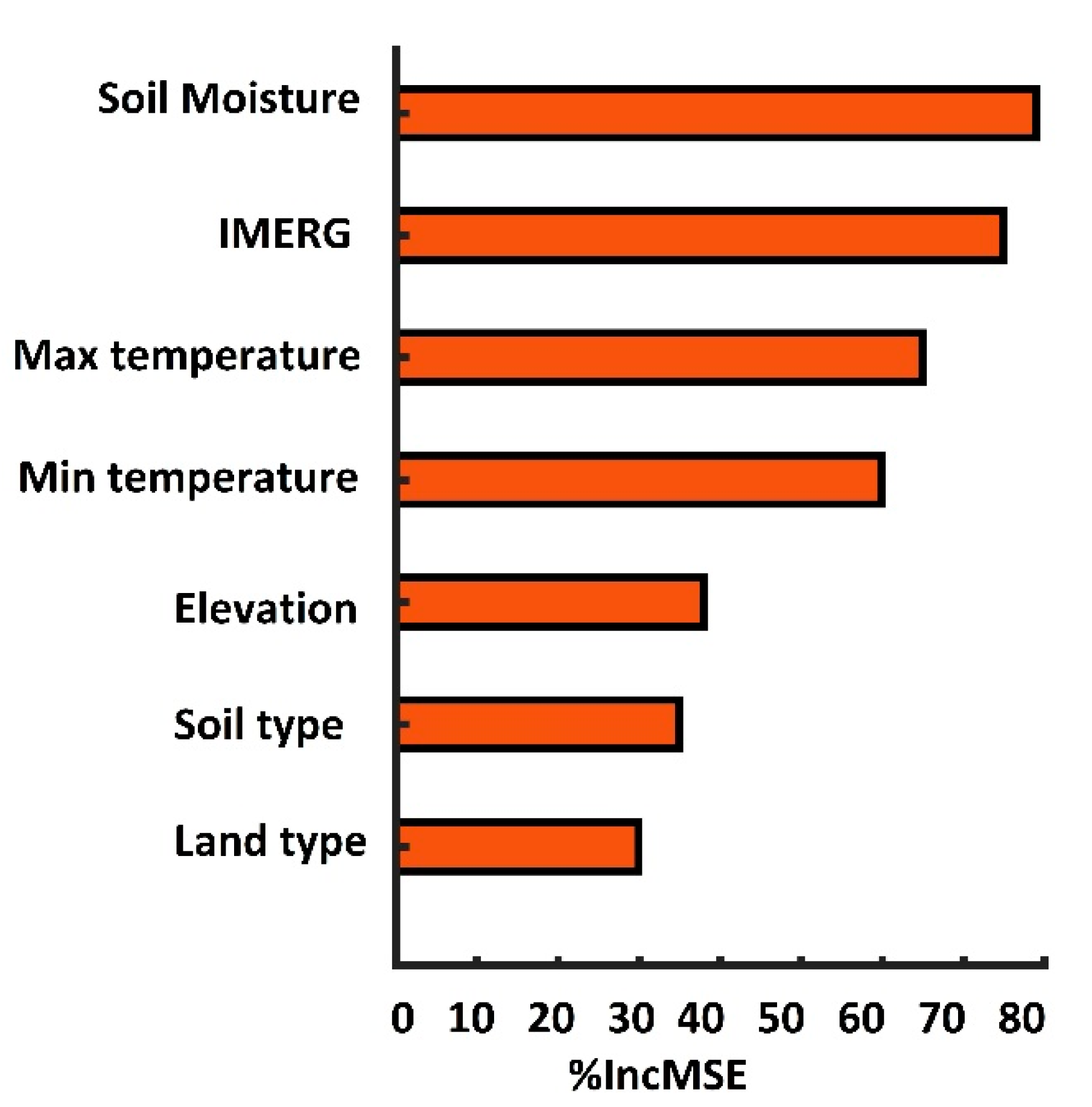
A variable importance experiment was conducted by calculating the magnitude of the percentage increase in mean square error (%IncMSE) of the model [52,93]. Higher magnitudes of %IncMSE show higher importance of the input features for the error model. The result from the variable importance experiment is displayed in Figure 6. The results showed that all features are comparatively important by producing promising %IncMSE values (0.3–0.8). The level of significance varies marginally for soil moisture, IMERG and temperature (%IncMSE values: 0.65–0.8) among the different variables. This sensitivity analysis also demonstrated that other variables are vital by producing decent %IncMSE values (0.3–0.4) for the error modeling.

4.2. Evaluation of Error Model Corrected Rainfall Rates

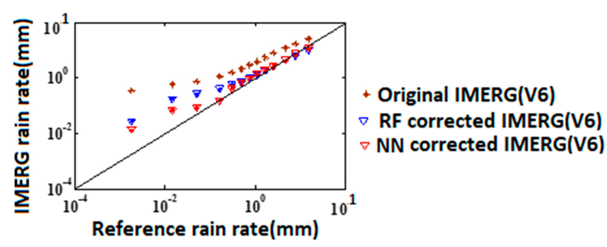
In this section, we used Quantile-vs.-Quantile (Q-Q) plot and the error metrics described in Section 3.2 (NCRMSE, MRE, U1, and U2) to compare machine learning-based error model performances. To compare the error-corrected IMERG(V6) precipitation estimates using the two different error models (NN and RF), the Q-Q plots of the original IMERG(V6), error-corrected IMERG(V6), and reference rain rates were produced for the test datasets, as shown in Figure 7. The figure displayed that the NN model corrections exhibited a slight improvement compared to the RF model.
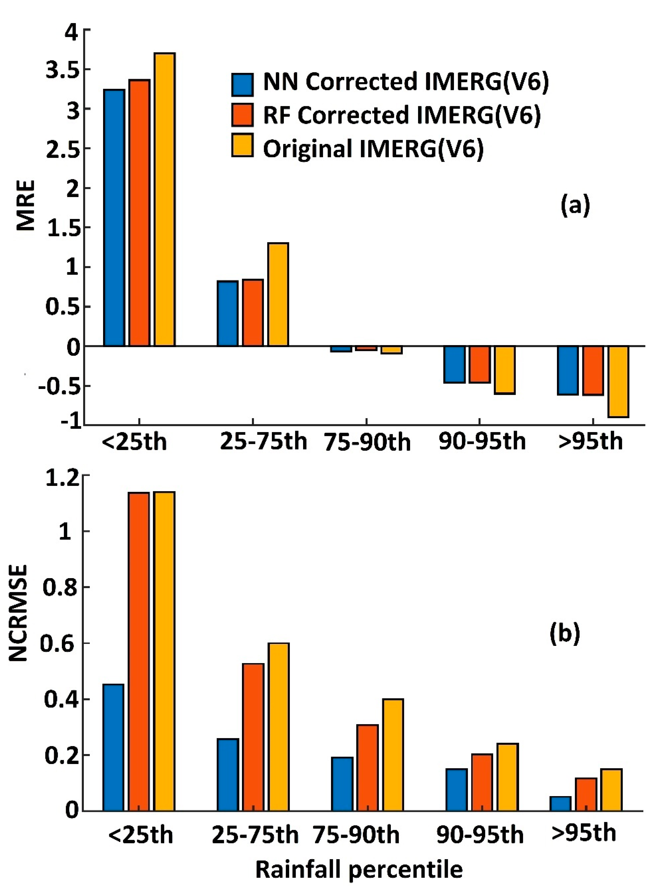
The performances of the models were also evaluated in terms of the mean relative error (MRE), as shown in Figure 8. MRE is calculated for five reference precipitation ranges: rainfall values in the range of <25th, 25th–75th, 75th–90th, 90th–95th, and >95th percentile. The results indicated that NN and RF were able to significantly reduce the systematic error for the >25th percentile. We found low systematic error values for both models corrected IMERG(V6) compared to original IMERG(V6) estimates, which indicated acceptable characterization of estimation uncertainty. The error-corrected IMERG(V6) product exhibited a slightly higher improvement in the NN technique by reducing systematic error compared to the RF model for all five reference precipitation ranges. For the >75th percentile, all individual rainfall datasets (original IMERG(V6), RF-corrected IMERG(V6), NN-corrected IMERG(V6)) showed underestimation. For the low rainfall (<25th), the systematic error (3.2–3.3) slightly reduced for both models, compared to the systematic error (3.7) of the original IMERG(V6). Moreover, the error metric difference ( Δ e r r o r ) considering MRE was estimated for the different reference precipitation ranges to show the performances of RF-corrected IMERG(V6), and NN-corrected IMERG(V6), (Table 3). The relative reduction of the systematic error for both model corrected IMERG(V6) is substantial (9–42%) with respect to original IMERG(V6).
The normalized centered root mean square error (NCRMSE) metric was examined precisely for the quantification of the performances of the estimates of IMERG. The results are summarized in Figure 8. The results showed that the random error reduced consistently in all products (original IMERG(V6), RF-corrected IMERG(V6), NN-corrected IMERG (V6) as the rainfall rate increased. Both models corrected IMERG(V6) and exhibited lower random error in comparison to the original IMERG(V6) for all precipitation ranges. The NN-corrected IMERG(V6) results exhibited a substantially higher improvement by producing lower random error compared to the RF model. Specifically, for the high rain rates (>95th percentile), the NN error model reported considerably reduced NCRMSE values (~0.05) compared to the RF error model. Similarly, for reference rainfall values in the moderate rainfall ranges (>25th percentile to <95th percentile), the results show that the NN-based corrections (NCRMSE: 0.15–0.20) bring IMERG estimates closer to the reference precipitation. Furthermore, the error metric difference ( Δ e r r o r ) considering NCRMSE for the different models are presented in Table 3. The NN-corrected IMERG(V6) showed substantial relative reduction of random error (37–65%) with respect to the original IMERG(V6) precipitation datasets over the study area. Similarly, RF-corrected IMERG(V6) produced a reasonable relative reduction of random error (~<21%) which also demonstrated the satisfactory performance of RF-corrected IMERG (V6) in comparison to original IMERG (V6). Overall, this study revealed a machine learning-based error model that leads to an advanced error characterization of IMERG precipitation estimation by the significant improvement of random and systematic error.
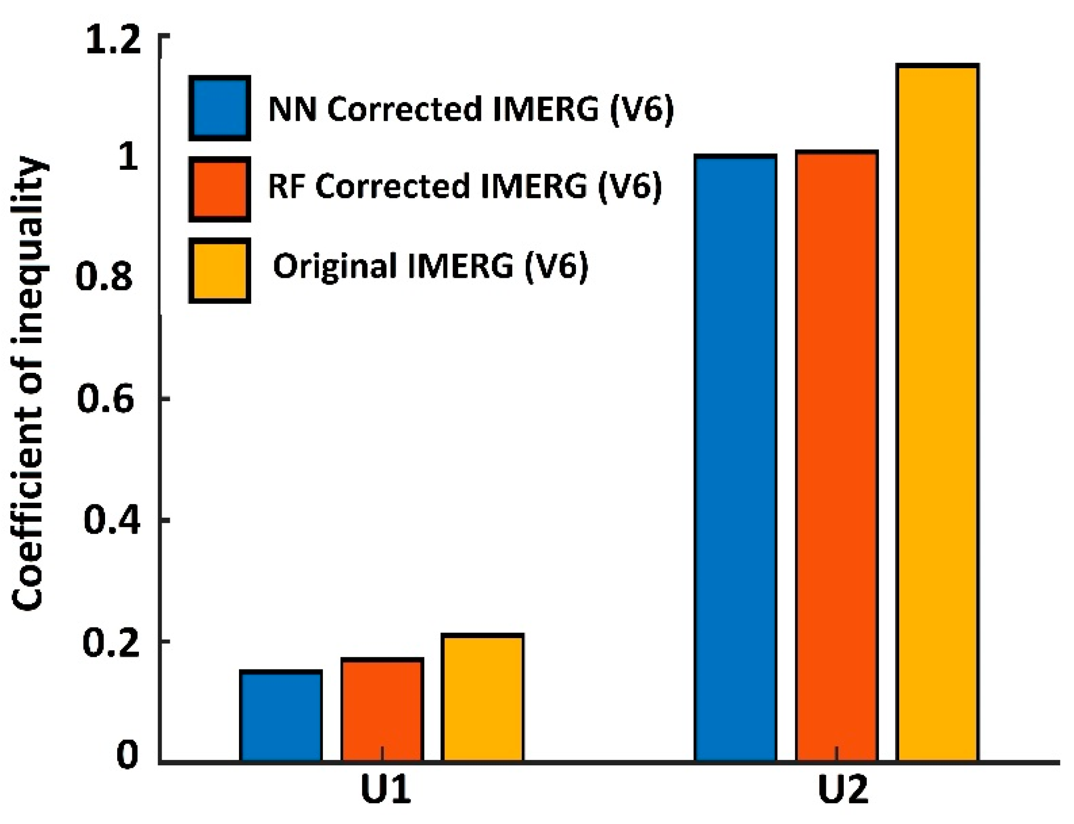
In addition, Theil’s inequality co-efficient (U1 and U2) values for the different models are shown in Figure 9. Theil’s inequality co-efficient, U1 marginally varied 0.15 to 0.17 for the two models, values which are less than the original IMERG(V6) produced U1 (0.21), as a function of magnitude which showed prominent performances in both models. The magnitude of U2 greater (lower) than 1 indicates less (more) accurate performance compared to the naïve approach. Moreover, both models also showed similar performances by producing U2 values close to ~1. Theil’s inequality co-efficient, U2 (1.15) for original IMERG(V6) is greater than both models. These results indicated that the model-corrected IMERG(V6) exhibited a slightly further improvement compared to the original IMERG(V6). Overall, the Theil’s inequality co-efficient results showed small relative improvements for the model-corrected IMERG(V6) compared to the original IMERG(V6).

4.3. Discussion

Two error models, the random forest (RF) and the neural network (NN), were evaluated based on quantitative error statistics (i.e., NCRMSE and MRE), and Theil’s “coefficient of inequality” statistics (U1 and U2). The systematic error for the models varied from overestimation to underestimation as the rain rate increased which is coherent to the findings of [3,14,19,20]. Moreover, the NN model showed promising performance for the moderate and high precipitation rate by displaying a high relative reduction of systematic error (23–37%).
Additionally, the NCRMSE metric was also assessed to quantify the effect of precipitation error modeling in reducing the random error component. The study showed that machine learning-based error models significantly reduced random error, and this reduction exhibited rainfall magnitude dependence. Specifically, NCRMSE for NN reduced (65%) considerably for the high rain rates (>95th percentile), showing a very high degree of agreement with reference precipitation which was consistent with findings by previous studies [14,15,33]. In addition, the RF and NN techniques considered elevation as a significant feature, which demonstrated the ability of the models to reduce the systematic and random error considerably in the study area. Overall, the performance of the machine learning-based precipitation estimates was consistent with findings by previous studies [14,15,33].
We would like to note that the results shown in Section 4.2 are based on the test dataset and showed improved results by significantly reducing random and systematic errors, which indicates that our model is successfully calibrated and could potentially be useful to predict the independent hydrometeorological dataset. The machine learning-based error models can manipulate the training data in such a way that the actual results expected from the untrained dataset can be quite different from the evaluated results using the training dataset [51,52,94]. Therefore, we considered the representation of extreme (>95th and <25th) precipitation values in the training and testing dataset to make sure that it covered the entire range of the dataset. Applying such a validation approach, the model has good skill on the independent test data in this analysis, which prevents overfitting by producing reliable results.

5. Conclusions

In this study, we investigated machine learning-based precipitation error modeling algorithms to improve the GPM IMERG precipitation product utilizing meteorological and land surface features (elevation, soil type, land type, soil moisture, and daily maximum and minimum temperature) with high-resolution in-situ precipitation rainfall data over the Brahmaputra river basin.
The comparison of NN and RF corrected rainfall values and the reference rainfall values were performed using Q-Q plots and showing satisfactory alignment along the 45-degree line. The error corrected IMERG(V6) results exhibited a slightly higher improvement by NN compared to the RF model. To investigate the accuracy of the error models, validation experiments based on the out-of-sample data approach were used. In terms of systematic and random error metrics, no significant differences were exhibited between two models (RF and NN). Generally, the machine learning-based model is expected not to capture very low and extremely high values successfully [14,93]. This is because the model accuracy is sensitive to sample size and the data representativeness in the training dataset [95,96]. Therefore, very large sample sizes are required for low and extremely high values to quantify the rate of convergence to the underlying cumulative distribution function. Results from quantitative error statistics are consistent in terms of the reduction of the random and systematic error for all the precipitation percentile ranges. This is an indication of how we successfully trained our model instead of overfitting.
The accurate estimation of rainfall in ungauged areas is an essential component to understand water resource systems efficiently. Therefore, extending this machine learning-based error modeling algorithm to the global scale and for other PMW precipitation estimates can be potentially useful. The improvements demonstrated by the error models with independent cross-validation approach indicate the transferability of the error model among complex terrains. Another possible extension of this study is to investigate uses of the PMW ensemble-based error predictions in integrated precipitation algorithms such as NOAA’s CMORPH techniques.

Author Contributions

For this research M.A.E.B. developed the precipitation error model, designed, and carried out the analysis of results, and wrote the paper. F.Y. co-designed the analysis of results and contributed to the development of the paper. N.K.B. contributed to the analysis of results and, together with S.H.R., and T.J.N. contributed to the interpretation of results and the writing of the paper. All authors have read and agreed to the published version of the manuscript.

Funding

This research received no external funding.

Acknowledgments

We gratefully acknowledge to GPM (https://gpm.nasa.gov/data-access/downloads/gpm) from where IMERG dataset was obtained for the analysis free of charge. We also acknowledge government organizations: Central Water Commission, India: http://cwc.gov.in/, Bangladesh Meteorological Department, Bangladesh: http://live3.bmd.gov.bd/, Bangladesh Water Development Board, Bangladesh: www.ffwc.gov.bd, Department of Hydrology and Meteorology, Nepal: https://www.dhm.gov.np/, for providing the in-situ data.

Conflicts of Interest

The authors declare no conflict of interest.

References

  1. Liu, Z. Comparison of versions 6 and 7 3-hourly TRMM multi-satellite precipitation analysis (TMPA) research products. Atmos. Res. 2015, 163, 91–101. [Google Scholar] [CrossRef] [Green Version]
  2. Sun, Q.; Miao, C.; Duan, Q.; Ashouri, H.; Sorooshian, S.; Hsu, K. A Review of Global Precipitation Data Sets: Data Sources, Estimation, and Intercomparisons. Rev. Geophys. 2018, 56, 79–107. [Google Scholar] [CrossRef] [Green Version]
  3. Liu, Z. Comparison of Integrated Multisatellite Retrievals for GPM (IMERG) and TRMM Multisatellite Precipitation Analysis (TMPA) Monthly Precipitation Products: Initial Results. J. Hydrometeorol. 2016, 17, 777–790. [Google Scholar] [CrossRef]
  4. Steinschneider, S.; Ray, P.; Rahat, S.H.; Kucharski, J. A Weather-Regime-Based Stochastic Weather Generator for Climate Vulnerability Assessments of Water Systems in the Western United States. Water Resour. Res. 2019, 55, 6923–6945. [Google Scholar] [CrossRef]
  5. Trenberth, K. Changes in precipitation with climate change. Clim. Res. 2011, 47, 123–138. [Google Scholar] [CrossRef] [Green Version]
  6. Huffman, G.J.; Bolvin, D.T.; Braithwaite, D.; Hsu, K.; Joyce, R.; Kidd, C.; Nelkin, E.J.; Xie, P. NASA Global Precipitation Measurement Integrated Multi-satellitE Retrievals for GPM (IMERG). Algorithm Theor. Basis Doc. 2015, 6, 30. [Google Scholar]
  7. Hou, A.Y.; Kakar, R.K.; Neeck, S.; Azarbarzin, A.A.; Kummerow, C.D.; Kojima, M.; Oki, R.; Nakamura, K.; Iguchi, T. The Global Precipitation Measurement Mission. Bull. Am. Meteorol. Soc. 2014, 95, 701–722. [Google Scholar] [CrossRef]
  8. Grecu, M.; Olson, W.S.; Munchak, S.J.; Ringerud, S.; Liao, L.; Haddad, Z.; Kelley, B.L.; McLaughlin, S.F. The GPM Combined Algorithm. J. Atmos. Ocean. Technol. 2016, 33, 2225–2245. [Google Scholar] [CrossRef]
  9. Smith, E.A.; Asrar, G.; Furuhama, Y.; Ginati, A.; Mugnai, A.; Nakamura, K.; Adler, R.F.; Chou, M.-D.; Desbois, M.; Durning, J.F.; et al. International Global Precipitation Measurement (GPM) Program and Mission: An Overview. In Measuring Precipitation from Space; Springer: Dordrecht, The Netherlands, 2007; pp. 611–653. [Google Scholar]
  10. Derin, Y.; Anagnostou, E.; Berne, A.; Borga, M.; Boudevillain, B.; Buytaert, W.; Chang, C.-H.; Delrieu, G.; Hong, Y.; Hsu, Y.C.; et al. Multiregional Satellite Precipitation Products Evaluation over Complex Terrain. J. Hydrometeorol. 2016, 17, 1817–1836. [Google Scholar] [CrossRef]
  11. Mei, Y.; Anagnostou, E.N.; Nikolopoulos, E.I.; Borga, M. Error Analysis of Satellite Precipitation Products in Mountainous Basins. J. Hydrometeorol. 2014, 15, 1778–1793. [Google Scholar] [CrossRef]
  12. Houze, R.A., Jr. Orographic effects on precipitating clouds. Rev. Geophys. 2012, 50, 289. [Google Scholar] [CrossRef]
  13. Roe, G.H. Orographic Precipitation. Annu. Rev. Earth Planet. Sci. 2005, 33, 645–671. [Google Scholar] [CrossRef]
  14. Bhuiyan, M.A.E.; Nikolopoulos, E.I.; Anagnostou, E.N.; Quintana-Seguí, P.; Barella-Ortiz, A. A nonparametric statistical technique for combining global precipitation datasets: Development and hydrological evaluation over the Iberian Peninsula. Hydrol. Earth Syst. Sci. 2018, 22, 1371–1389. [Google Scholar] [CrossRef] [Green Version]
  15. Ehsan Bhuiyan, M.A.; Nikolopoulos, E.I.; Anagnostou, E.N. Machine Learning–Based Blending of Satellite and Reanalysis Precipitation Datasets: A Multiregional Tropical Complex Terrain Evaluation. J. Hydrometeorol. 2019, 20, 2147–2161. [Google Scholar] [CrossRef]
  16. Ehsan Bhuiyan, M.A.; Nikolopoulos, E.I.; Anagnostou, E.N.; Polcher, J.; Albergel, C.; Dutra, E.; Fink, G.; Martínez-de la Torre, A.; Munier, S. Assessment of precipitation error propagation in multi-model global water resource reanalysis. Hydrol. Earth Syst. Sci. 2019, 23, 1973–1994. [Google Scholar] [CrossRef] [Green Version]
  17. Casse, C.; Gosset, M.; Peugeot, C.; Pedinotti, V.; Boone, A.; Tanimoun, B.A.; Decharme, B. Potential of satellite rainfall products to predict Niger River flood events in Niamey. Atmos. Res. 2015, 163, 162–176. [Google Scholar] [CrossRef]
  18. Yong, B.; Liu, D.; Gourley, J.J.; Tian, Y.; Huffman, G.J.; Ren, L.; Hong, Y. Global View Of Real-Time Trmm Multisatellite Precipitation Analysis: Implications For Its Successor Global Precipitation Measurement Mission. Bull. Am. Meteorol. Soc. 2015, 96, 283–296. [Google Scholar] [CrossRef]
  19. Sharifi, E.; Steinacker, R.; Saghafian, B. Assessment of GPM-IMERG and Other Precipitation Products against Gauge Data under Different Topographic and Climatic Conditions in Iran: Preliminary Results. Remote Sens. 2016, 8, 135. [Google Scholar] [CrossRef] [Green Version]
  20. Tan, M.; Ibrahim, A.; Duan, Z.; Cracknell, A.; Chaplot, V. Evaluation of Six High-Resolution Satellite and Ground-Based Precipitation Products over Malaysia. Remote Sens. 2015, 7, 1504–1528. [Google Scholar] [CrossRef] [Green Version]
  21. Asong, Z.E.; Razavi, S.; Wheater, H.S.; Wong, J.S. Evaluation of Integrated Multisatellite Retrievals for GPM (IMERG) over Southern Canada against Ground Precipitation Observations: A Preliminary Assessment. J. Hydrometeorol. 2017, 18, 1033–1050. [Google Scholar] [CrossRef]
  22. Gebregiorgis, A.S.; Kirstetter, P.; Hong, Y.E.; Gourley, J.J.; Huffman, G.J.; Petersen, W.A.; Xue, X.; Schwaller, M.R. To What Extent is the Day 1 GPM IMERG Satellite Precipitation Estimate Improved as Compared to TRMM TMPA-RT? J. Geophys. Res. Atmos. 2018, 123, 1694–1707. [Google Scholar] [CrossRef]
  23. Kim, K.; Park, J.; Baik, J.; Choi, M. Evaluation of topographical and seasonal feature using GPM IMERG and TRMM 3B42 over Far-East Asia. Atmos. Res. 2017, 187, 95–105. [Google Scholar] [CrossRef]
  24. Murali Krishna, U.V.; Das, S.K.; Deshpande, S.M.; Doiphode, S.L.; Pandithurai, G. The assessment of Global Precipitation Measurement estimates over the Indian subcontinent. Earth Space Sci. 2017, 4, 540–553. [Google Scholar] [CrossRef]
  25. Sungmin, O.; Foelsche, U.; Kirchengast, G.; Fuchsberger, J.; Tan, J.; Petersen, W.A. Evaluation of GPM IMERG Early, Late, and Final rainfall estimates using WegenerNet gauge data in southeastern Austria. Hydrol. Earth Syst. Sci. 2017, 21, 6559–6572. [Google Scholar]
  26. Sunilkumar, K.; Yatagai, A.; Masuda, M. Preliminary Evaluation of GPM-IMERG Rainfall Estimates Over Three Distinct Climate Zones With APHRODITE. Earth Space Sci. 2019, 6, 1321–1335. [Google Scholar] [CrossRef] [Green Version]
  27. Tang, G.; Ma, Y.; Long, D.; Zhong, L.; Hong, Y. Evaluation of GPM Day-1 IMERG and TMPA Version-7 legacy products over Mainland China at multiple spatiotemporal scales. J. Hydrol. 2016, 533, 152–167. [Google Scholar] [CrossRef]
  28. Tian, F.; Hou, S.; Yang, L.; Hu, H.; Hou, A. How does the evaluation of GPM IMERG rainfall product depend on gauge density and rainfall intensity? J. Hydrometeorol. 2019, 19, 339–349. [Google Scholar] [CrossRef]
  29. Xu, R.; Tian, F.; Yang, L.; Hu, H.; Lu, H.; Hou, A. Ground validation of GPM IMERG and TRMM 3B42V7 rainfall products over southern Tibetan Plateau based on a high-density rain gauge network. J. Geophys. Res. Atmos. 2017, 122, 910–924. [Google Scholar] [CrossRef]
  30. Wang, S.; Liu, J.; Wang, J.; Qiao, X.; Zhang, J. Evaluation of GPM IMERG V05B and TRMM 3B42V7 Precipitation Products over High Mountainous Tributaries in Lhasa with Dense Rain Gauges. Remote Sens. 2019, 11, 2080. [Google Scholar] [CrossRef] [Green Version]
  31. Chen, F.; Li, X. Evaluation of IMERG and TRMM 3B43 Monthly Precipitation Products over Mainland China. Remote Sens. 2016, 8, 472. [Google Scholar] [CrossRef] [Green Version]
  32. Islam, M.A. Statistical comparison of satellite-retrieved precipitation products with rain gauge observations over Bangladesh. Int. J. Remote Sens. 2018, 39, 2906–2936. [Google Scholar] [CrossRef] [Green Version]
  33. Bhuiyan, M.A.E.; Anagnostou, E.N.; Kirstetter, P.-E. A Nonparametric Statistical Technique for Modeling Overland TMI (2A12) Rainfall Retrieval Error. IEEE Geosci. Remote Sens. Lett. 2017, 14, 1898–1902. [Google Scholar] [CrossRef]
  34. Biemans, H.; Hutjes, R.W.A.; Kabat, P.; Strengers, B.J.; Gerten, D.; Rost, S. Effects of Precipitation Uncertainty on Discharge Calculations for Main River Basins. J. Hydrometeorol. 2009, 10, 1011–1025. [Google Scholar] [CrossRef]
  35. Jiang, H.; Qiang, M.; Lin, P.; Wen, Q.; Xia, B.; An, N. Framing the Brahmaputra River hydropower development: Different concerns in riparian and international media reporting. Water Policy 2017, 19, 496–512. [Google Scholar] [CrossRef]
  36. Zawahri, N.A. International rivers and national security: The Euphrates, Ganges-Brahmaputra, Indus, Tigris, and Yarmouk rivers1. Nat. Resour. Forum 2008, 32, 280–289. [Google Scholar] [CrossRef]
  37. Biba, S. Desecuritization in China’s Behavior towards Its Transboundary Rivers: The Mekong River, the Brahmaputra River, and the Irtysh and Ili Rivers. J. Contemp. China 2013, 23, 21–43. [Google Scholar] [CrossRef] [Green Version]
  38. Feng, Y.; Wang, W.; Liu, J. Dilemmas in and Pathways to Transboundary Water Cooperation between China and India on the Yaluzangbu-Brahmaputra River. Water 2019, 11, 2096. [Google Scholar] [CrossRef] [Green Version]
  39. Ray, P.A.; Yang, Y.-C.E.; Wi, S.; Khalil, A.; Chatikavanij, V.; Brown, C. Room for improvement: Hydroclimatic challenges to poverty-reducing development of the Brahmaputra River basin. Environ. Sci. Policy 2015, 54, 64–80. [Google Scholar] [CrossRef] [Green Version]
  40. Oliveira, R.; Maggioni, V.; Vila, D.; Porcacchia, L. Using Satellite Error Modeling to Improve GPM-Level 3 Rainfall Estimates over the Central Amazon Region. Remote Sens. 2018, 10, 336. [Google Scholar] [CrossRef] [Green Version]
  41. Seyyedi, H.; Anagnostou, E.N.; Kirstetter, P.-E.; Maggioni, V.; Yang, H.; Gourley, J.J. Incorporating Surface Soil Moisture Information in Error Modeling of TRMM Passive Microwave Rainfall. IEEE Trans. Geosci. Remote Sens. 2014, 52, 6226–6240. [Google Scholar] [CrossRef]
  42. Hossain, F.; Anagnostou, E.N. A two-dimensional satellite rainfall error model. IEEE Trans. Geosci. Remote Sens. 2006, 44, 1511–1522. [Google Scholar] [CrossRef]
  43. Hossain, F.; Anagnostou, E.N. Assessment of a Multidimensional Satellite Rainfall Error Model for Ensemble Generation of Satellite Rainfall Data. IEEE Geosci. Remote Sens. Lett. 2006, 3, 419–423. [Google Scholar] [CrossRef]
  44. Maggioni, V.; Reichle, R.H.; Anagnostou, E.N. The Effect of Satellite Rainfall Error Modeling on Soil Moisture Prediction Uncertainty. J. Hydrometeorol. 2011, 12, 413–428. [Google Scholar] [CrossRef]
  45. Maggioni, V.; Anagnostou, E.N.; Reichle, R.H. The impact of model and rainfall forcing errors on characterizing soil moisture uncertainty in land surface modeling. Hydrol. Earth Syst. Sci. 2012, 16, 3499–3515. [Google Scholar] [CrossRef] [Green Version]
  46. Schanze, J.; Schwarze, R.; Cartensen, D.; Deilmann, C. Analyzing and managing uncertain futures of large-scale fluvial flood risk systems. Presented at the Managing Flood Risk, Reliability and Vulnerability, Proceedings of 4th International Symposium on Flood Defence, Toronto, ON, Canada, 6–8 May 2008. [Google Scholar]
  47. Croley, T.E., II. Weighted Parametric Operational Hydrology Forecasting. In Proceedings of the World Water & Environmental Resources Congress, Philadelphia, PA, USA, 23–26 June 2003; American Society of Civil Engineers: ‎Reston, VA, USA. [Google Scholar]
  48. Brown, J.D.; Seo, D.-J. A Nonparametric Postprocessor for Bias Correction of Hydrometeorological and Hydrologic Ensemble Forecasts. J. Hydrometeorol. 2010, 11, 642–665. [Google Scholar] [CrossRef] [Green Version]
  49. Mujumdar, P.P.; Ghosh, S. Climate Change Impact on Hydrology and Water Resources. ISH J. Hydraul. Eng. 2008, 14, 1–17. [Google Scholar] [CrossRef]
  50. Yenigun, K.; Ecer, R. Overlay mapping trend analysis technique and its application in Euphrates Basin, Turkey. Meteorol. Appl. 2012, 20, 427–438. [Google Scholar] [CrossRef]
  51. Meinshausen, N. Quantile regression forests. J. Mach. Learn 2006, 7, 983–999. [Google Scholar]
  52. Breiman, L. Random forests, machine learning 45. J. Clin. Microbiol. 2001, 2, 199–228. [Google Scholar]
  53. Chipman, H.A.; George, E.I.; McCulloch, R.E. Bayesian CART Model Search. J. Am. Stat. Assoc. 1998, 93, 935–948. [Google Scholar] [CrossRef]
  54. Chipman, H.A.; George, E.I.; McCulloch, R.E. BART: Bayesian additive regression trees. Ann. Appl. Stat. 2010, 4, 266–298. [Google Scholar] [CrossRef]
  55. Barnard, E.; Cole, R.A. A neural-net training program based on conjugate-radient optimization. CSETech 1989, 199. [Google Scholar]
  56. Dougherty, M.S.; Cobbett, M.R. Short-term inter-urban traffic forecasts using neural networks. Int. J. Forecast. 1997, 13, 21–31. [Google Scholar] [CrossRef]
  57. Gunrey, K. An Introduction to Neural Networks; UCL Press Limited: London, UK, 1997. [Google Scholar]
  58. Kala, A.; Vaidyanathan, S.G. Prediction of Rainfall Using Artificial Neural Network. In Proceedings of the 2018 International Conference on Inventive Research in Computing Applications (ICIRCA), Coimbatore, India, 11–12 July 2018. [Google Scholar]
  59. Sulaiman, J.; Wahab, S.H. Heavy Rainfall Forecasting Model Using Artificial Neural Network for Flood Prone Area. In IT Convergence and Security 2017; Springer: Singapore, 2017; pp. 68–76. [Google Scholar]
  60. Choubin, B.; Zehtabian, G.; Azareh, A.; Rafiei-Sardooi, E.; Sajedi-Hosseini, F.; Kişi, Ö. Precipitation forecasting using classification and regression trees (CART) model: A comparative study of different approaches. Environ. Earth Sci. 2018, 77, 314. [Google Scholar] [CrossRef]
  61. Kashiwao, T.; Nakayama, K.; Ando, S.; Ikeda, K.; Lee, M.; Bahadori, A. A neural network-based local rainfall prediction system using meteorological data on the Internet: A case study using data from the Japan Meteorological Agency. Appl. Soft Comput. 2017, 56, 317–330. [Google Scholar] [CrossRef]
  62. Bhuiyan, M.A.E.; Begum, F.; Ilham, S.J.; Khan, R.S. Advanced wind speed prediction using convective weather variables through machine learning application. Appl. Comput. Geosci. 2019, 1, 100002. [Google Scholar]
  63. Nashwan, M.S.; Shahid, S. Symmetrical uncertainty and random forest for the evaluation of gridded precipitation and temperature data. Atmos. Res. 2019, 230, 104632. [Google Scholar] [CrossRef]
  64. Herman, G.R.; Schumacher, R.S. Money Doesn’t Grow on Trees, but Forecasts Do: Forecasting Extreme Precipitation with Random Forests. Mon. Weather Rev. 2018, 146, 1571–1600. [Google Scholar] [CrossRef]
  65. Afshin, S.; Fahmi, H.; Alizadeh, A.; Sedghi, H.; Kaveh, F. Long term rainfall forecasting by integrated artificial neural network-fuzzy logic-wavelet model in Karoon basin. Sci. Res. Essays 2011, 6, 1200–1208. [Google Scholar]
  66. Azadi, S.; Sepaskhah, A.R. Annual precipitation forecast for west, southwest, and south provinces of Iran using artificial neural networks. Theor. Appl. Climatol. 2011, 109, 175–189. [Google Scholar] [CrossRef]
  67. Sigaroodi, S.K.; Chen, Q.; Ebrahimi, S.; Nazari, A.; Choobin, B. Long-term precipitation forecast for drought relief using atmospheric circulation factors: A study on the Maharloo Basin in Iran. Hydrol. Earth Syst. Sci. 2014, 18, 1995–2006. [Google Scholar] [CrossRef] [Green Version]
  68. Nishat, B.; Rahman, S.M.M. Water Resources Modeling of the Ganges-Brahmaputra-Meghna River Basins Using Satellite Remote Sensing Data1. JAWRA J. Am. Water Resour. Assoc. 2009, 45, 1313–1327. [Google Scholar] [CrossRef]
  69. Beran, M.A. Recent advances in statistical flood estimation techniques. In Flood studies Report—Five Years on; Thomas Telford Publishing: London, UK, 1981; pp. 25–32. [Google Scholar]
  70. Hossain, F.; Katiyar, N.; Hong, Y.; Wolf, A. The emerging role of satellite rainfall data in improving the hydro-political situation of flood monitoring in the under-developed regions of the world. Nat. Hazards 2007, 43, 199–210. [Google Scholar] [CrossRef]
  71. Shiklomanov, A.I.; Lammers, R.B.; Vörösmarty, C.J. Widespread decline in hydrological monitoring threatens Pan-Arctic Research. EosTrans. Am. Geophys. Union 2002, 83, 13. [Google Scholar] [CrossRef]
  72. Sterling, S.M.; Ducharne, A.; Polcher, J. The impact of global land-cover change on the terrestrial water cycle. Nat. Clim. Chang. 2012, 3, 385–390. [Google Scholar] [CrossRef]
  73. Verma, S.; Mukherjee, A.; Choudhury, R.; Mahanta, C. Brahmaputra river basin groundwater: Solute distribution, chemical evolution and arsenic occurrences in different geomorphic settings. J. Hydrol. Reg. Stud. 2015, 4, 131–153. [Google Scholar] [CrossRef] [Green Version]
  74. Yang, Y.C.E.; Wi, S.; Ray, P.A.; Brown, C.M.; Khalil, A.F. The future nexus of the Brahmaputra River Basin: Climate, water, energy and food trajectories. Glob. Environ. Chang. 2016, 37, 16–30. [Google Scholar] [CrossRef] [Green Version]
  75. Bajracharya, S.R.; Palash, W.; Shrestha, M.S.; Khadgi, V.R.; Duo, C.; Das, P.J.; Dorji, C. Systematic Evaluation of Satellite-Based Rainfall Products over the Brahmaputra Basin for Hydrological Applications. Adv. Meteorol. 2015, 2015, 1–17. [Google Scholar] [CrossRef]
  76. Shrestha, M.S.; Artan, G.A.; Bajracharya, S.R.; Sharma, R.R. Using satellite-based rainfall estimates for streamflow modelling: Bagmati Basin. J. Flood Risk Manag. 2008, 1, 89–99. [Google Scholar] [CrossRef]
  77. Peel, M.C.; Finlayson, B.L.; McMahon, T.A. Updated world map of the Köppen-Geiger climate classification. Hydrol. Earth Syst. Sci. 2007, 11, 1633–1644. [Google Scholar] [CrossRef] [Green Version]
  78. Papa, F.; Frappart, F.; Malbeteau, Y.; Shamsudduha, M.; Vuruputur, V.; Sekhar, M.; Ramillien, G.; Prigent, C.; Aires, F.; Pandey, R.K.; et al. Satellite-derived surface and sub-surface water storage in the Ganges–Brahmaputra River Basin. J. Hydrol. Reg. Stud. 2015, 4, 15–35. [Google Scholar] [CrossRef] [Green Version]
  79. Huffman, G.J.; Stocker, E.F.; Bolvin, D.T.; Nelkin, E.J.; Tan, J. GPM IMERG Late Precipitation L3 1 Day 0.1 Degree x 0.1 Degree V06; Andrey, S., Greenbelt, M.D., Eds.; Goddard Earth Sciences Data and Information Services Center (GES DISC), 2019. Available online: https://disc.gsfc.nasa.gov/datasets/GPM_3IMERGDF_06/summary (accessed on 1 May 2020).
  80. Reichle, R.; De Lannoy, G.; Koster, R.D.; Crow, W.T.; Kimball, J.S.; Liu, Q. SMAP L4 Global 3-hourly 9 km EASE-Grid Surface and Root Zone Soil Moisture Geophysical Data, version 4; NASA National Snow and Ice Data Center Distributed Active Archive Center: Boulder, CO, USA, 2018. [Google Scholar] [CrossRef]
  81. Wan, Z.S.; Hulley, H.G. MOD11C1 MODIS/Terra Land Surface Temperature/Emissivity Daily L3 Global 0.05Deg CMG V006. NASA EOSDIS Land Processes DAAC. last access date: May 26 2020, distributed in netCDF format by the Integrated Climate Data Center (ICDC, icdc.cen.uni-hamburg.de); University of Hamburg: Hamburg, Germany, 2015. [Google Scholar] [CrossRef]
  82. Earth Resources Observation and Science (EROS) Center. Global Land Cover Characterization (GLCC) [Data set]. U.S. Geological Survey, 2017. [CrossRef]
  83. FAO/IIASA/ISRIC/ISS-CAS/JRC. Harmonized World Soil Database (Version 1.1); FAO: Rome, Italy; IIASA: Laxenburg, Austria, 2009; Available online: http://www.fao.org/3/a-aq361e.pdf (accessed on 1 May 2020).
  84. Biswas, N.K.; Hossain, F. A scalable open-source web-analytic framework to improve satellite-based operational water management in developing countries. J. Hydroinformatics 2017, 20, 49–68. [Google Scholar] [CrossRef]
  85. Cutler, A.; Cutler, D.R.; Stevens, J.R. Random Forests. In Ensemble Machine Learning; Springer: New York, NY, USA, 2012; pp. 157–175. [Google Scholar]
  86. Pal, M. Random forest classifier for remote sensing classification. Int. J. Remote Sens. 2005, 26, 217–222. [Google Scholar] [CrossRef]
  87. Erb, R.J. Introduction to Backpropagation Neural Network Computation. Pharm. Res. 1993, 10, 165–170. [Google Scholar] [CrossRef]
  88. Hopfield, J.J. Neural networks and physical systems with emergent collective computational abilities. Proc. Natl. Acad. Sci. 1982, 79, 2554–2558. [Google Scholar] [CrossRef] [Green Version]
  89. Günther, F.; Fritsch, S. neuralnet: Training of Neural Networks. R J. 2010, 2, 30. [Google Scholar] [CrossRef] [Green Version]
  90. Riedmiller, M. Rprop-Description and Implementation Details; Technical Report; University of Karlsruhe: Karlsruhe, Germany, 1994. [Google Scholar]
  91. Intrator, O.; Intrator, N. Using neural nets for interpretation of nonlinear models. In Proceedings of the Statistical Computing Section, San Francisco, CA, USA, 8–12 August 1993; American Statistical Society: Alexandria, VA, USA, 1993; pp. 244–249. [Google Scholar]
  92. Bliemel, F. Theil’s Forecast Accuracy Coefficient: A Clarification. J. Mark. Res. 1973, 10, 444. [Google Scholar] [CrossRef]
  93. Yang, F.; Watson, P.; Koukoula, M.; Anagnostou, E.N. Enhancing Weather-Related Power Outage Prediction by Event Severity Classification. IEEE Access 2020, 8, 60029–60042. [Google Scholar] [CrossRef]
  94. Ajiboye, A.R.; Abdullah-Arshah, R.; Hongwu, Q. Evaluating the effect of dataset size on predictive model using supervised learning technique. Int. J. Comput. Syst. Softw. Eng. 2015, 1, 75–84. [Google Scholar] [CrossRef]
  95. Mondal, A.R.; Bhuiyan, M.A.E.; Yang, F. Advancement of weather-related crash prediction model using nonparametric machine learning algorithms. SN Appl. Sci. 2020, 2, 1372. [Google Scholar] [CrossRef]
  96. Yang, F.; Wanik, D.W.; Cerrai, D.; Bhuiyan, M.A.E.; Anagnostou, E.N. Quantifying uncertainty in machine learning-based power outage prediction model training: A tool for sustainable storm restoration. Sustainability 2020, 12, 1525. [Google Scholar] [CrossRef] [Green Version]
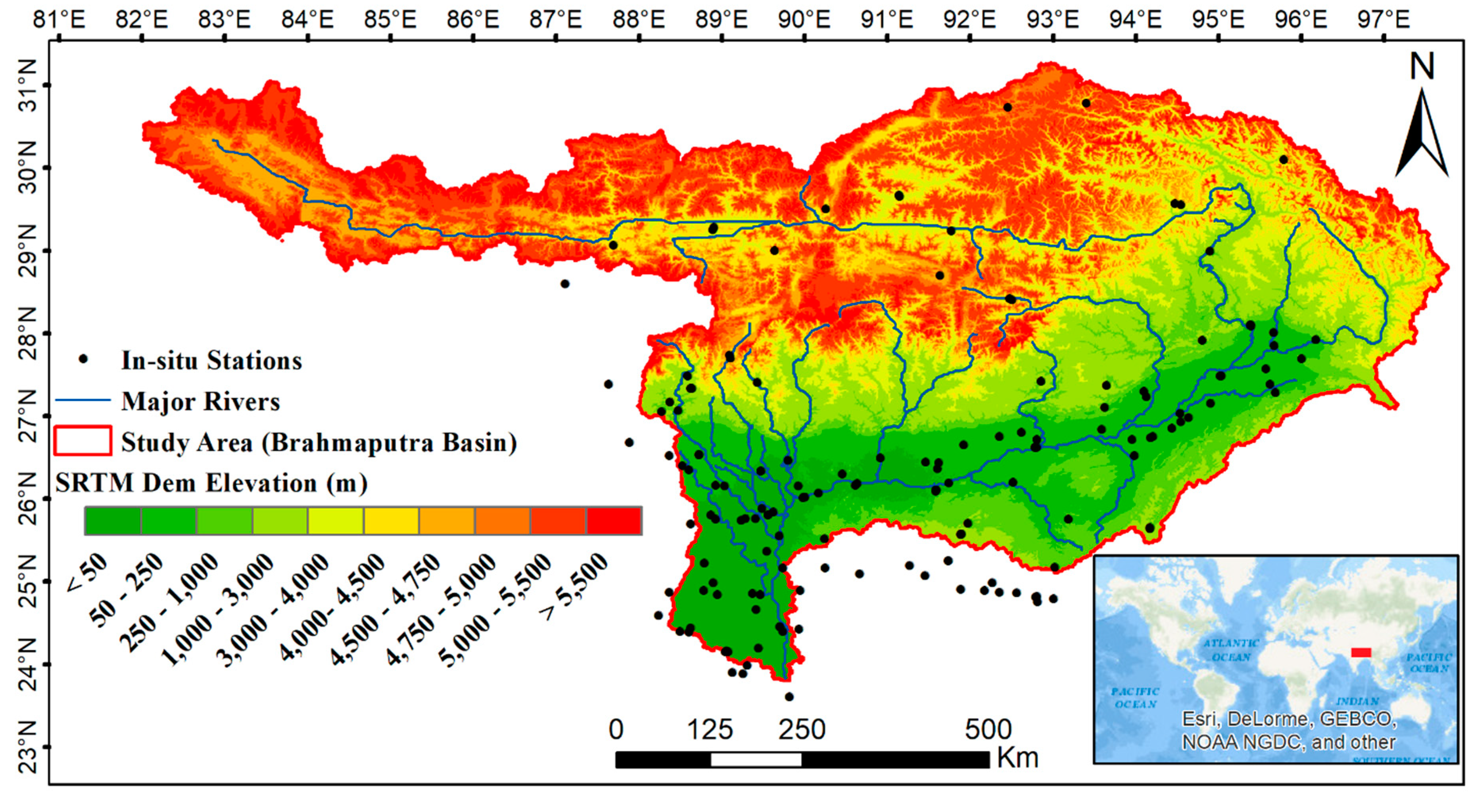
Figure 1. Study Area (Brahmaputra River Basin) with the Shuttle Radar Topographic Mission, SRTM (1 arc second spatial resolution) elevation variation. Solid circles represent gauge locations. The red marked area in the inset map for location reference.
Forecasting 02 00014 g001
Figure 2. Schematic representation of the prediction process for this study.
Forecasting 02 00014 g002
Figure 3. Mean square residual plotted against the number of trees in the random forest.
Forecasting 02 00014 g003
Figure 4. A schematic representation of the random forests (RF).
Forecasting 02 00014 g004
Figure 5. A schematic representation of the neural network (NN).
Forecasting 02 00014 g005
Figure 6. Variable importance plot, where %IncMSE is the percentage increase in mean square error.
Forecasting 02 00014 g006
Figure 7. Quantile-vs.-Quantile (Q-Q) diagram of original and model corrected IMERG(V6) rainfall vs. reference rainfall.
Forecasting 02 00014 g007
Figure 8. (a) Mean relative error of original IMERG(V6) and model corrected IMERG(V6) rain rate; (b) Normalized centered root mean square error of original IMERG(V6) and model corrected IMERG(V6) rain rate.
Forecasting 02 00014 g008
Figure 9. Theil’s inequality co-efficient of original IMERG(V6) and model corrected IMERG(V6) rain rate.
Forecasting 02 00014 g009
Table 1. Datasets used in this study area.
Data TypeProductSpatial ResolutionTemporal ResolutionCoverageReference/Source
Meteorological DataSatellite-based Precipitation0.1° by 0.1°30 minGlobal: 90° N–90° Shttps://gpm.nasa.gov/data-access/downloads/gpm
Soil Moisture9 km EASE-Grid; Resampled to 0.1° by 0.1°3 hGlobal: 85.044° N–85.044° Shttps://nsidc.org/data/SPL4SMGP/versions/4
Daily Maximum and Minimum Temperature0.05° by 0.05° Climate Modelling Grid; Resampled to 0.1° by 0.1°DailyGlobal: 90° N–90° Shttps://lpdaac.usgs.gov/products/mod11c1v006/
In-situ PrecipitationVarious; Resampled to 0.1° by 0.1°DailyBrahmaputra Basin Regionhttp://cwc.gov.in/
http://live3.bmd.gov.bd/
http://www.dhm.gov.np/
Land Surface DataSRTM DEM1 arc second Globalhttps://earthexplorer.usgs.gov/
USGS Land Cover data1 km grid Globalhttps://earthexplorer.usgs.gov/
FAO Harmonized World Soil Database30 arc second Globalhttp://www.fao.org/soils-portal/soil-survey/soil-maps-and-databases/harmonized-world-soil-database-v12/en/
Table 2. The tuned hyperparameters for RF and NN models.
Random ForestNeural Network
R Package “randomForest”R Package “neuralnet”
mtry = 5Hidden nodes = 5
ntree = 1000learning rate = 0.01
stepmax = 108
linear.output = TRUE
Table 3. Relative reduction of systematic error and random error with respect to original IMERG(V6) rain rate. Results are presented for different precipitation ranges.
Rainfall PercentileRelative Reduction of Systematic Error Relative Reduction of Random Error
NNRFNNRF
<25th12%9%60%0%
25–75th37%36%57%12%
75–90th24%42%52%23%
90–95th23%23%37%16%
>95th32%32%65%21%