Article

On Underdispersed Count Kernels for Smoothing Probability Mass Functions

by
Célestin C. Kokonendji
1,2,*,†,
Sobom M. Somé
3,4,*,†,
Youssef Esstafa
5 and
Marcelo Bourguignon
6
1
Laboratoire de Mathématiques de Besançon UMR 6623 CNRS-UBFC, Université Bourgogne Franche-Comté, 16 Route de Gray, CEDEX, 25030 Besançon, France
2
Laboratoire de Mathématiques et Connexes de Bangui, Université de Bangui, Av. des Martyrs, Bangui B.P. 908, Central African Republic
3
Laboratoire d’Analyse Numérique Informatique et de BIOmathématique, Université Joseph KI-ZERBO, Ouagadougou 03 BP 7021, Burkina Faso
4
Laboratoire Sciences et Techniques, Université Thomas SANKARA, Ouagadougou 12 BP 417, Burkina Faso
5
Laboratoire Manceau de Mathématiques, Le Mans Université, Avenue Olivier Messiaen, CEDEX 09, 72085 Le Mans, France
6
Departamento de Estatística, Universidade Federal do Rio Grande do Norte, Natal 59078-970, Brazil
*
Authors to whom correspondence should be addressed.
These authors contributed equally to this work.
Stats 2023, 6(4), 1226-1240; https://doi.org/10.3390/stats6040076
Submission received: 8 October 2023 / Revised: 29 October 2023 / Accepted: 2 November 2023 / Published: 4 November 2023
(This article belongs to the Special Issue Statistics, Analytics, and Inferences for Discrete Data)

Abstract

:
Only a few count smoothers are available for the widespread use of discrete associated kernel estimators, and their constructions lack systematic approaches. This paper proposes the mean dispersion technique for building count kernels. It is only applicable to count distributions that exhibit the underdispersion property, which ensures the convergence of the corresponding estimators. In addition to the well-known binomial and recent CoM-Poisson kernels, we introduce two new ones such the double Poisson and gamma-count kernels. Despite the challenging problem of obtaining explicit expressions, these kernels effectively smooth densities. Their good performances are pointed out from both numerical and comparative analyses, particularly for small and moderate sample sizes. The optimal tuning parameter is here investigated by integrated squared errors. Also, the added advantage of faster computation times is really very interesting. Thus, the overall accuracy of two newly suggested kernels appears to be between the two old ones. Finally, an application including a tail probability estimation on a real count data and some concluding remarks are given.

1. Introduction

Nonparametric statistics use (discrete) asymmetric kernel methods to capture and visually represent complex relationships between variables that cannot be effectively captured by symmetric kernels. A common practice now is to employ kernels whose support coincides with the nature or support of the dataset, whether it is count, categorical, bounded, unbounded, continuous, left or right skewed, and so on. See, for example, refs. [1,2,3] for smoothing of probability mass, probability density, and regression functions with environmental, econometric and financial applications, among others. Discrete smoothing of probability mass functions in the case of counts and categoricals has not been studied as extensively as its continuous counterparts, primarily due to the limited options for suitable kernels. There are two main classes of discrete associated kernels. The first, called of the “second order” (with δ = 0 in Definition 1), includes kernels whose estimators are consistent and asymptotically tend towards the true function as for the Dirac kernel. Such discrete (asymmetric and symmetric) kernels are, for instance, triangular [4], Aitchison–Aitken or Dirac Uniform [5], Wang and Van Ryzin [6], and the recently proposed CoM-Poisson [7,8]; see also [3]. The second class, so-called of the “first order” (with δ ( 0 , 1 ) in Definition 1), generally contains the binomial kernel [4] appropriate for small and moderate sample sizes for which the corresponding estimators do not converge. The previous discrete kernels are suitable for categorical data, with the exception of the binomial and CoM-Poisson kernels, which are appropriated for count data. Additionally, all these associated kernels are typically underdispersed, i.e., its variance is less than the expectation; on the contrary, the equidispersed Poisson and overdispersed negative binomial kernels are not recommended for count smoothings; see [4], the authors of which make intensive simulations that highlight the superiority of these underdispersed discrete smoothers versus equi-/over-dispersed ones. The reader can also refer to [9,10] for some applications of discrete kernels in survey sampling and the model specification test, respectively, and more generally to Li and Racine [11]. Here is the precise definition of a discrete associated kernel; see, e.g., Esstafa et al. [8].
Definition 1. 
Let T R be the discrete support of the probability mass function (pmf) f to be estimated, x T a target point and h > 0 a bandwidth. A parameterized pmf K x , h ( · ) on the discrete support S x R is called “discrete associated kernel” if the following conditions are satisfied:
x S x , lim h 0 E ( Z x , h ) = x a n d lim h 0 Var ( Z x , h ) = δ [ 0 , 1 ) ,
where Z x , h denotes the discrete random variable with pmf K x , h ( · ) .
We suppose X 1 , X 2 , , X n is a sample of independent and identically distributed (iid) discrete random variables with a pmf f defined on T R . The usual discrete associated kernel estimator of f is generally not a pmf. This is particularly true for some discrete associated-kernels such as the binomial, triangular, and CoM-Poisson, where the total mass of the corresponding estimator does not necessarily equal one; see, e.g., [12]. Specifically, one can express both estimators as follows:
f ^ n ( x ) = f ˜ n ( x ) C n , x T ,
with
f ˜ n ( x ) = 1 n i = 1 n K x , h n ( X i ) and C n = x T f ˜ n ( x ) > 0 ,
where ( h n ) n 1 is an arbitrary sequence of positive smoothing (or tuning) parameters that satisfies lim n h n = 0 , while K x , h n ( · ) is a suitably chosen discrete kernel function. For the following three kernels of Dirac, Aitchison and Aitken [5] and Wang and Van Rizin [6], it is easy to check that C n = 1 , and therefore f ˜ n = f ^ n . Esstafa et al. [8] recently demonstrated the effectiveness of the normalized version (1) compared to the unnormalized one (2) with illustrations using the existing count (convergent or not-convergent) smoothers: binomial and CoM-Poisson, respectively. We here use the standardized version (1) for all. In nonparametric (discrete or continous) kernel estimation, the tuning (smoothing) parameter plays a crucial role in preventing overfitting and underfitting. Bandwidth selection methods can be categorized into three families: global bandwidths for all smoothers, adaptive for continuous kernels, and local ones for discrete (count and categorical) estimators. For example, Chu et al. [13] proposed a rule-of-thumb approach, Harfouche et al. [1] utilized cross-validations, and Somé et al. [2] emploed a local Bayesian method. It is important to note that smoothers using local bandwidths, which vary according to each estimation point, are referred to as “balloon estimators”, while adaptive bandwidths, varying for each data point, are known as “sample-point estimators”.
In this paper, we propose two new count kernels, namely the double Poisson and the gamma-count, derived from their underdispersed distributions parts. These additions enrich the list of existing count kernels, such as binomial and CoM-Poisson. Specifically, they reinforce the roster of “first-order” kernels, which exclusively contains the CoM-Poisson, and whose smoothers are consistent and asymptotically tend towards the Dirac kernel. Their construction is performed through the mean dispersion technique which appears as a variant of the mode dispersion method [12] in continuous cases. The rest of the paper is organized as follows. In Section 2, we recall some underdispersed count distributions including the double Poisson and gamma-count which have some specific properties in their expressions. Section 3 is devoted to building the double Poisson and gamma-count kernels after introducing the mean dispersion method of consruction and despite some approximations in their properties. Section 4 presents the main results from our simulation studies and then an application on a count dataset on development days of insect pests on Hura trees. Final remarks are made in Section 5. Some other underdispersed count distributions and local Bayesian bandwidth selection are mentionned in Appendix A and Appendix B in relation to their feasibility.

2. Some Properties of Underdispersed Count Distributions

In this section we recall three count distributions, namely the double Poisson, the gamma-count and the CoM-Poisson, which are underdispersed according to a part of their parameters. Before building their corresponding associated kernels to satisfy Definition 1, we point out their main properties needed (pmf, mean and variance) even if they are not generally in closed-form expressions. Thus, approximation and computation approaches are used for a better understanding of the parameters.
  • The double Poisson pmf is defined by
    p ( y ; λ , γ ) : = K λ , γ D P ( y ) = k ( λ , γ ) γ 1 / 2 e γ λ e y y y y ! e λ y γ λ , y = 0 , 1 , 2 , ,
    with
    1 k ( λ , γ ) = y = 0 γ 1 / 2 e γ λ e y y y y ! e λ y γ λ 1 + 1 γ 12 γ λ 1 + 1 γ λ
    and where γ > 0 is the dispersion parameter and λ > 0 . The mean and variance do not have closed-form expressions but they can be approximated, respectively, by
    E Y λ and Var Y λ γ .
    We note that the values 0 < γ < 1 , γ = 1 and γ > 1 correspond to overdispersion, equidispersion and underdispersion, respectively. See Efron [14] and Toledo et al. [15] for further details.
  • The gamma-count pmf for the number of events within the time interval ( 0 , T ) is given, with α , β > 0 , through
    p ( y ; α , β ) = K α , β G C ( y ) = G ( y α , β T ) G ( α ( y + 1 ) , β T ) y = 0 , 1 , 2 , ,
    with the cumulative distribution function
    G ( y α , β T ) = 1 Γ ( y α ) 0 β T u y α 1 exp ( u ) d u
    and for y = 0 , G ( 0 , β T ) = 1 and T can be set to one, without loss of generality. The parameter α > 0 is such that α > 1 and 0 < α < 1 refer to underdispersion or overdispersion, respectively. Here, the mean and variance are not available in closed form but they can be computed through
    E Y = y = 1 G y α , β T and Var ( Y ) = y = 1 y 2 K α , β G C ( y ) [ E Y ] 2 .
    See Winkelmann [16] for further details, Zeviani et al. [17] for an application to regression model, and also [15].
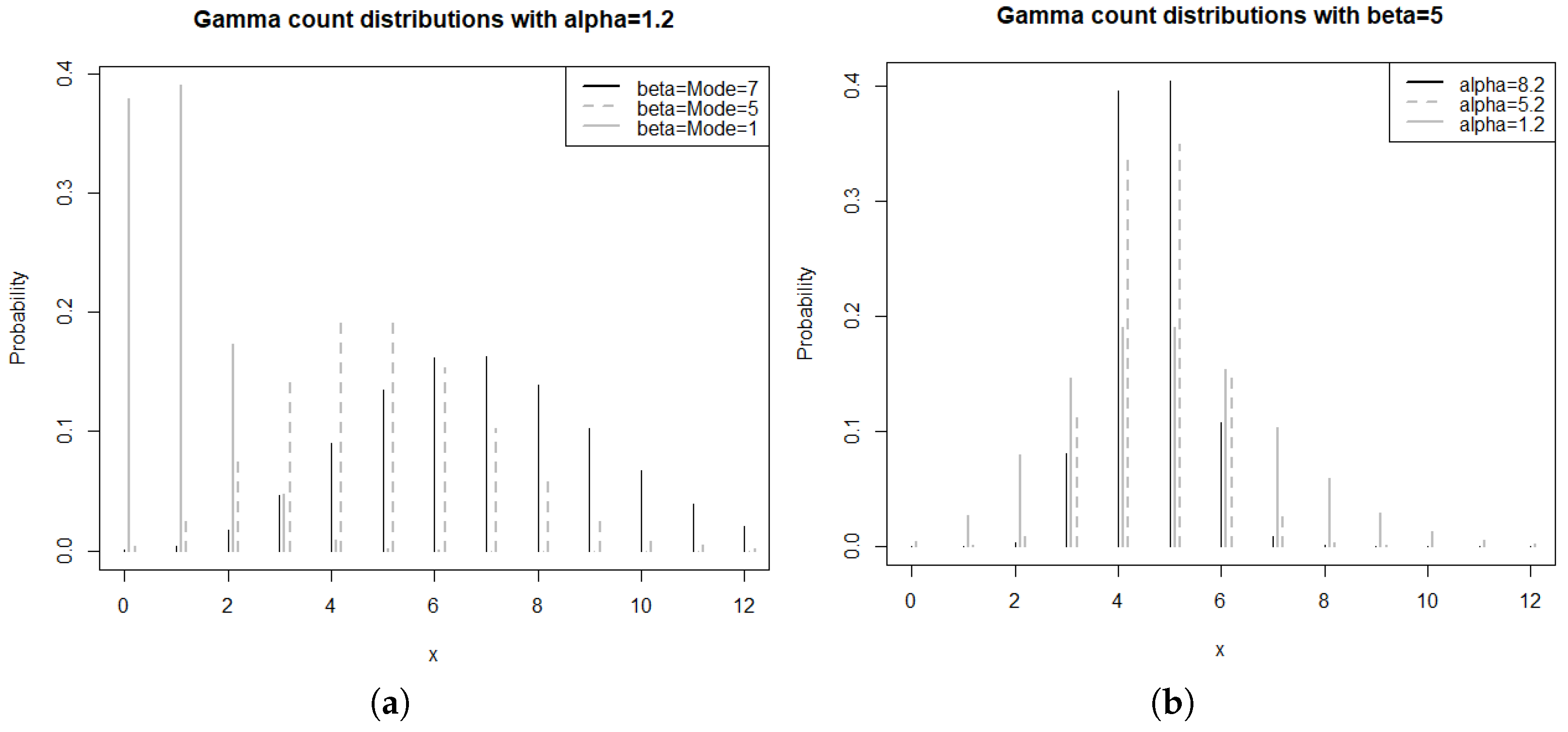
    Numerically and from Figure 1, we can observe that the mean E Y of the gamma-count distribution is almost always a constant around β ; specifically, by zooming in, we notice that the shape of the curve is logarithmic or approximately linear in α > 0 for fixed β > 0 . The same fact is observed for its mode, as shown in Figure 2. We also note that Figure 2 highlights the role of β > 0 as a shape or location parameter and α > 0 as a scale or dispersion parameter of the gamma-count distribution. Hence, the variance of the gamma-count distribution can be seen as a function of α > 0 .
  • The CoM-Poisson distribution with location parameter μ 0 and dispersion parameter ν > 0 ( ν > 1 for underdispersion) such that its pmf p ( · ; μ , ν ) is defined by
    p ( y ; μ , ν ) : = K μ , 1 / ν C M P ( y ) = λ ( μ , ν ) y ( y ! ) ν 1 D ( λ ( μ , ν ) , ν ) , y N ,
    where function λ : = λ ( μ , ν ) is the solution to equation
    z = 0 λ ( μ , ν ) z ( z ! ) 1 / h ( z μ ) = 0 ,
    and it is used to define the normalizing constant D ( λ ( μ , ν ) , ν ) = y = 0 [ λ ( μ , ν ) ] y / ( y ! ) ν . Then,
    E ( Y ) = μ and Var Y = 1 ν λ ( μ , ν ) 1 / ν + O λ ( μ , ν ) 1 / ν ,
    when { λ ( μ , ν ) } 1 / ν as ν . See, for example, ref. [8] for some references.
Also, we can refer to Appendix A for some underdispersed count distributions such as the BerPoi, generalized Poisson, an underdispersed Poisson, the BerG and the hyper-Poisson, for which their corresponding count associated kernels are inconclusive.

3. Associated Kernel Versions

We introduce in this section the notion of the mean dispersion-ready pmf, a new method inspired by the mode dispersion technique (see, for example, [12]) and adapted to the discrete setting. This method allows construction of discrete associated kernels and is applicable to underdispersed count distributions.
Definition 2. 
A mean dispersion-ready pmf K θ is a underdispersed parametrized pmf with discrete support S θ R , θ Θ R 2 , such that K θ has moments of second order with mode m R and admitting dispersion parameter D.
Remark 1. 
Let K θ be a mean dispersion-ready pmf on S θ R . The following two assertions are satisfied:
(i) 
the mode m of K θ always belongs to S θ ;
(ii) 
if μ is the mean of K θ , then K θ ( m ) K θ ( μ ) , where · denotes the integer part.
In order to create discrete associated kernels from an underdispersed unimodal mean dispersion-ready pmf K θ defined on S θ , the mean dispersion method requires, if it exists, an explicit solution of the following system of equations:
θ ( m , D ) = ( x , h ) .
It should be noted that this construction may not always be possible, and alternative methods can be found in [8,12,18].
Now, we illustrate the use of (6) in four examples such both new double Poisson and gamma-count kernels, as well as the old CoM-Poisson and binomial kernels.
Example 1. 
The double Poisson kernel of the second order and underdispersed for any h ( 0 , 1 ) is defined on S x = T = N for each x N ,
K x , h D P ( z ) = k ( x + h , 1 / h ) h 1 / 2 e ( x + h ) / h e z z z z ! e ( x + h ) z ( x + h ) / h , z = 0 , 1 , 2 , ,
where k ( x + h , 1 / h ) is the normalizing constant. It comes from (3) with the reparametrization of the system ( λ , γ ) = ( x + h , 1 / h ) which implies
E Z x , h D P x + h x a n d Var Z x , h D P ( x + h ) h 0
as h 0 , where Z : = Z x , h D P is the count random variable associated to this double Poisson kernel.
Example 2. 
The gamma-count kernel, which exhibits the underdispersion phenomenon for any h ( 0 , 1 ) , is derived from (4) with parametrization ( α , β ) = ( 1 / h , x + h ) . It is defined on S x = T = N for each x N and any h ( 0 , 1 ) by
K x , h G C ( z ) = G ( z / h , ( x + h ) T ) G ( ( z + 1 ) / h , ( x + h ) T ) , z = 0 , 1 , 2 ,
From the analyses of Figure 1 and Figure 2, the mean and mode of the associated gamma-count random variable Z : = Z x , h G C are around x + h , which therefore tend to a neighborhood of x when h 0 . Also, one can observe that Var Z x , h G C 0 as h 0 .
Example 3. 
The CoM-Poisson kernel of the second order and underdispersed for any h ( 0 , 1 ) is defined with S x = T = N for each x N ,
K x , h C M P ( z ) = λ ( x , 1 / h ) z ( z ! ) 1 / h D λ ( x , 1 / h ) , 1 / h 1 ,
where D ( λ ( x , 1 / h ) , 1 / h ) = z = 0 [ λ ( x , 1 / h ) ] z / ( z ! ) 1 / h is the normalizing constant and λ : = λ ( x , 1 / h ) represents a function of x and 1 / h given by the solution of
z = 0 λ ( x , 1 / h ) z ( z ! ) 1 / h ( z x ) = 0 .
One can refer to [7,8] for further details. This construction implies that E Z x , h C M P = x and
Var Z x , h C M P = λ ( x , 1 / h ) h h + O λ ( x , 1 / h ) h 0 as h 0 .
Example 4. 
The first-order and underdispersed binomial kernel is introduced by Kokonendji and Senga Kiessé [4] as follows: S x = { 0 , 1 , , x + 1 } for each x N = T and h ( 0 , 1 ) ,
K x , h B ( z ) = ( x + 1 ) ! z ! ( x + 1 z ) ! x + h x + 1 z 1 h x + 1 x + 1 z
with E Z x , h B = x + h x as h 0 and
Var Z x , h B = ( x + h ) ( 1 h ) x + 1 x x + 1 ( 0 , 1 ) as h 0 .
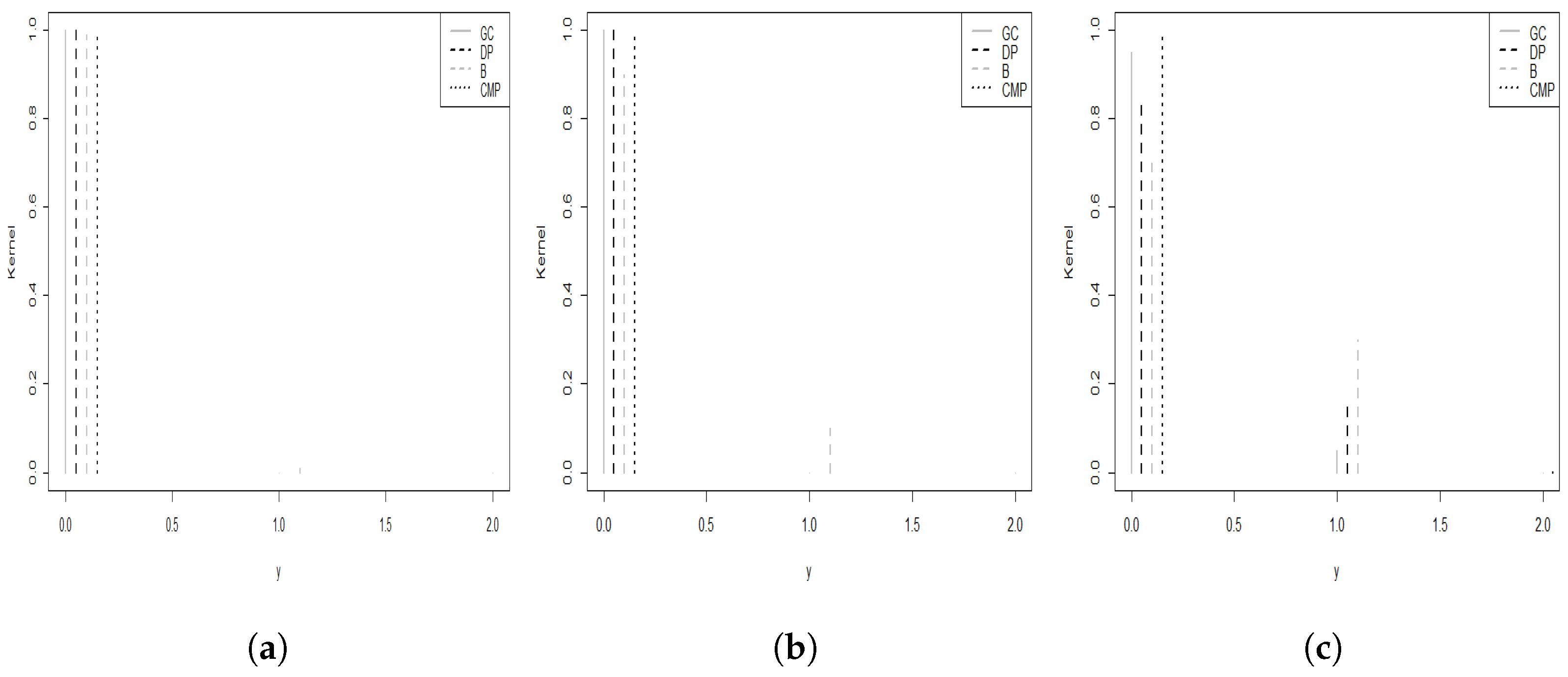
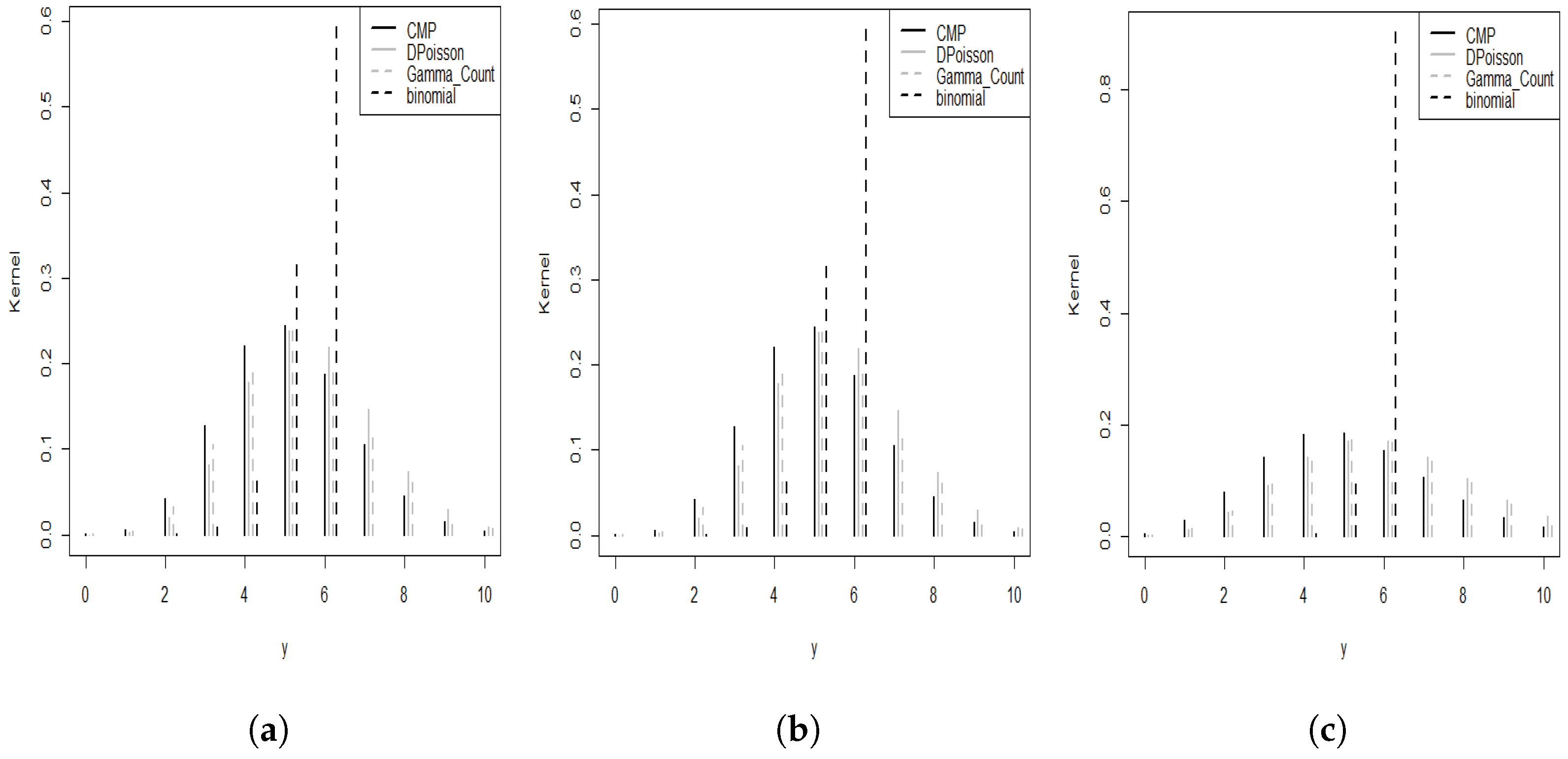
Figure 3 and Figure 4 show different behaviours of these four underdispersed count kernels at the origin x = 0 and at x = 5 , respectively, according to three values of the bandwidth h > 0 . Hence, the two newly suggested count kernels appear to be better competitors to the second-order CoM-Poisson kernel compared to the binomial one.

4. Simulation Studies and an Application to Real Data

The purpose of all numerical studies conducted here is to investigate the performances of the two new double Poisson and gamma-count kernels alongside the classical binomial and CoM-Poisson smoothers derived from (1) and (2). Computations are conducted on a 2.30 GHz PC using the R 4.2.1 software [19]. The previous smoothers are fitted using the rmutil, Ake and mpcmp packages [20,21,22], respectively. The corresponding four underdispersed count kernel estimators are assessed by employing integrated squared error (ISE) method to determine the optimal bandwidth parameter
h i s e = arg min h ( 0 , 1 ) x T f ^ n ( x ) f ( x ) 2 .
In fact, the usual cross-validation (data-driven) technique does not converge in simulations and real data for the proposed kernel estimator: double Poisson and gamma-count. The reader can refer, for others methods, to Chu [13] for the plug-in method, Harfouche et al. [1] for cross-validation and to Kokonendji and Senga Kiéssé [4] for mean integrated squared errors.
In this study, we examine the performances of four count smoothers using count simulated datasets under four different scenarios denoted by A, B, C, and D. These scenarios are chosen to assess how well the estimators handle zero inflation, unimodality and multimodality. We evaluate the effectiveness of the smoothers by analyzing the empirical estimates of the ISE, specifically
I S E ^ n : = 1 N s i m t = 1 N s i m x T f ^ n ( x ) f ( x ) 2 ,
where N s i m is the number of replications and n denotes the sample size.
  • Scenario A is generated by using the Poisson distribution
    f A ( x ) = 8 x e 8 x ! , x N ;
  • Scenario B comes from the zero-inflated Poisson distribution
    f B ( x ) = 7 10 1 { x = 0 } + 3 10 × 10 x e 10 x ! 1 N { 0 } ( x ) ;
  • Scenario C is from a mixture of two Poisson distributions
    f C ( x ) = 2 5 × 0 . 5 x e 0.5 x ! + 3 5 × 8 x e 8 x ! , x N ;
  • Scenario D comes from a mixture of three Poisson distributions
    f D ( x ) = 3 5 × 10 x e 10 x ! + 1 5 × 22 x e 22 x ! + 1 5 × 50 x e 50 x ! , x N .
Table 1 presents the computation times required to perform all ISE bandwidth selection techniques (7) for gamma-count, double Poisson, binomial and CoM-Poisson smoothers based on a single replication of sample sizes ranging from n = 20 to 500 for the target function C. For all sample sizes, the results show that the CoM-Poisson is the most time consuming followed by the double Poisson smoother mainly due to the normalizing constant in their expressions, (5) and (3), respectively. As the sample sizes increase, the binomial kernel outperforms in terms of CPU times due to its support S x = { 0 , 1 , , x } , whereas the gamma-count kernel becomes the second quickest due to the integrals in its expression.
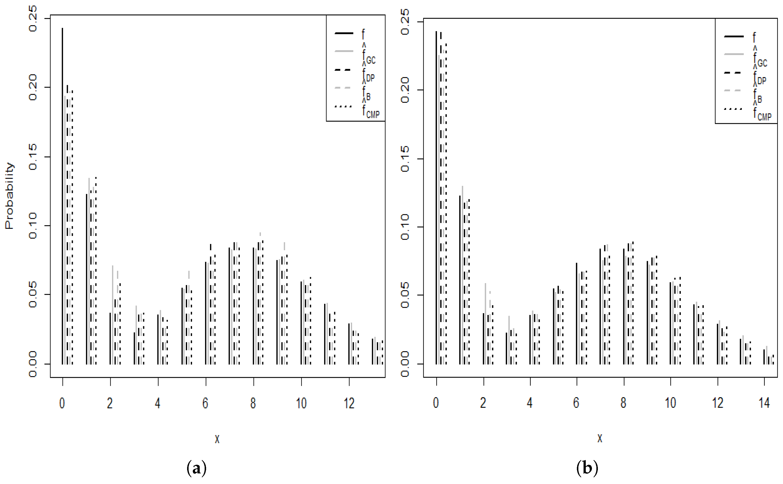
Figure 5 depicts the true pmf and the smoothing ones using gamma-count, double Poisson, binomial and CoM-Poisson kernels with respect to Scenario C, and for one replication. The graphs show that, in general, the two new underdispersed count kernel estimators are accurate.
Table 2 exhibits some empirical values of I S E n , obtained through ISE bandwidth selection (7) using N = 500 as number of replications, according to the four Scenarios A, B, C and D and with respect to sample sizes n = 10 , 25 , 50 , 100 , 250 , 500 . Then, several behaviours emerge. As the sample sizes increase, the smoothings improve for all smoothers. As expected, the binomial kernel is the least efficient since it is of the first order. The three others have comparable performances. The two new count kernels, namely double Poisson and gamma-count, are slightly more precise than the CoM-Poisson one, notably for small and medium sample sizes (i.e., n 100 ) while the latter is the best for large sample sizes. Additionally, approximations made for the moments of the gamma-count distribution (4) may help clarify the performance discrepancy between the two new kernels for larger sample sizes. Finally, from a purely practical perspective, Table 1 and Table 2 highlight the following ranking in performances: double Poisson, gamma-count and CoM-Poisson.
Now, we apply these four underdispersed count kernels for smoothing the real count dataset on development days of insect pests on Hura trees with moderate sample size n = 51 ; see also [8]. Practical performances are here examined via the empirical I S E method (7) and the empirical criterion of I S E :
h i s e 0 = arg min h ( 0 , 1 ) x T f ^ n ( x ) f 0 ( x ) 2 and I S E ^ 0 : = x T N f ^ n ( x ) f 0 ( x ) 2 ,
where f 0 ( · ) is the empirical or naive estimator. The double Poisson and the CoM-Poisson kernels are comparable and appear to be the best with h i s e 0 D P = 0.001 , I S E ^ 0 D P = 0.00031657 and h i s e 0 C M P = 0.006 , I S E ^ 0 C M P = 0.00034531 followed by the binomial smoother with h i s e 0 B = 0.001 and I S E ^ 0 B = 0.01232621 and finally the gamma-count smoother with h i s e 0 G C = 0.012 and I S E ^ 0 G C = 0.01287723 .
Figure 6 offers their graphical representations. We also evaluate the practical upper tail probability P ( X 32 ) suitable for applied statisticians. Then, these tail probabilities are estimated to be 0.1569 , 0.1949 , 0.1568 , 0.1510 and 0.1572 for the empirical frequency f 0 , gamma-count, double Poisson, binomial and CoM-Poisson kernel estimations, respectively. Although the double Poisson and the CoM-Poisson have similar performances, we recommend, again, the first one, which is more flexible and much faster; see Table 1.

5. Summary and Final Remarks

We introduced two novel underdispersed count kernels, specifically the double Poisson and gamma-count ones. They were developed using the proposed mean dispersion method. Also, we considered the integrated squared error method (7) to select as quickly and efficiently as possible the bandwidth of their corresponding estimations. Through simulation experiments and real count data analysis, we demonstrated that these kernels perform better than the binomial kernel, while falling between the CoM-Poisson kernel smoothing (which performs the best) and the binomial kernel (which performs the worst). Although the CoM-Poisson and double Poisson kernels have similar performances, we strongly recommend using the latter due to its significantly lower time consumption and its flexibility from some closed-form expressions.
We note that any underdispersed count distribution cannot always lead to its corresponding associated kernel; see Appendix A and also [23,24]. It would also be better to improve the bandwidth selection with data-driven methods; Appendix B mentions the direction for the local Bayesian bandwidth selection. In addition, an important fact for smoothing a pmf on T = { k , k + 1 , } with k 1 is to consider, for instance, the k-shifted version of any underdispersed count kernel. In fact, the two main properties of the associated kernel, as recalled in Definition 1, are first to adapt the support S of the kernel to T and second to maintain the variance property which tends to δ [ 0 , 1 ) as h 0 .

Author Contributions

Conceptualization, C.C.K. and S.M.S.; methodology, C.C.K. and S.M.S.; software, S.M.S.; validation, C.C.K. and S.M.S.; formal analysis, C.C.K. and S.M.S.; investigation, S.M.S.; resources, C.C.K. and S.M.S.; data curation, C.C.K. and S.M.S.; writing—original draft preparation, C.C.K. and S.M.S.; writing—review and editing, C.C.K., S.M.S., Y.E. and M.B.; visualization, C.C.K. and S.M.S.; supervision, C.C.K.; funding acquisition: C.C.K.; project administration: C.C.K., S.M.S. All authors have read and agreed to the published version of the manuscript.

Funding

This research was funded, for the first author, by “Brazilian-French Network in Mathematics”.

Institutional Review Board Statement

Not applicable.

Informed Consent Statement

Not applicable.

Data Availability Statement

All data used in the study are publicly available.

Acknowledgments

Part of this paper was written during the visit of the first author to the Department of Statistics, Universidade Federal do Rio Grande do Norte, Natal, RN, Brasil which is supported by grant from “Brazilian-French Network in Mathematics”. The authors are grateful to the Associate Editor and three anonymous referees for their constructive comments.

Conflicts of Interest

The authors declare no conflict of interest.

Abbreviations

The following abbreviations are used in this manuscript:
cmpCoM-Poisson
dpDouble Poisson
gcgamma-count
iidIndependent and identically distributed
ISEIntegrated squared error
pmfProbability mass functions

Appendix A. Some Other Underdispersed Count Distributions for Kernels Attempts

We provide five count distributions, namely BerPoi, generalized Poisson, underdispersed Poisson, BerG, and hyper-Poisson, which can exhibit the underdispersion property and have closed-form expressions for their pmf, mean, and variance. However, it is not possible to construct their corresponding associated kernels. Thus, an alternative approach to the proposed mean dispersion method may be necessary.
  • The BerPoi distribution has its pmf,
    p ( y ; α , λ ) : = K α , λ B P ( y ) = 1 α + α y λ e λ λ y y ! , y = 0 , 1 , ,
    with 0 < α < 1 and λ > 0 . Its mean and variance are, respectively,
    E ( Y ) : = μ = α + λ and Var ( Y ) : = σ 2 = α ( 1 α ) + λ .
    Bourguignon et al. [25] propose a reparametrization by mean μ = α + λ and dispersion index ϕ = 1 α 2 / ( λ + α ) ; that is, α = μ ( 1 ϕ ) and λ = μ μ ( 1 ϕ ) with μ > 0 and 0 < ϕ < 1 . It follows from this parametrization that
    E ( Y ) : = μ and Var ( Y ) : = μ ϕ
    and
    p ( y ; μ , ϕ ) : = K μ , ϕ B P ( y ) = 1 μ ( 1 ϕ ) + y μ ( 1 ϕ ) μ μ ( 1 ϕ ) × e μ + μ ( 1 ϕ ) ( μ μ ( 1 ϕ ) ) y y ! y = 0 , 1 , ,
    with conditions μ > 0 and 0 < min ( μ , 1 / μ ) < ϕ < 1 to ensure (A1) being underdispersed and a proper pmf.
  • The generalized Poisson (GP) is defined through its pmf as
    p ( y ; θ , δ ) : = K θ , δ G P ( y ) = θ θ + δ y y 1 e θ δ y y ! , y = 0 , 1 , 2 , ,
    with θ > 0 and max 1 , θ / 4 < δ < 1 ; see Harris et al. [26]. The corresponding mean and variance are given by
    μ = E Y = θ 1 δ , Var Y i = θ ( 1 δ ) 3 = 1 ( 1 δ ) 2 E Y = ϕ E Y .
    We thus obtain underdispersion for δ < 0 .
  • The pmf of the so-called Underdispersed Poisson distribution of Singh et al. [27] is given, for θ > 0 and λ > 0 , by
    p ( y ; λ , θ ) : = K λ , θ U P ( y ) = e λ λ y 1 ( λ + θ y ) ( 1 + θ ) y ! , y = 0 , 1 , 2 , ,
    with
    E ( Y ) : = μ = λ + θ 1 + θ and Var ( Y ) : = σ 2 = λ + θ ( 1 + θ ) 2 .
  • The BerG distribution is defined by
    p ( y ; π , θ ) : = K π , θ B G ( y ) = ( 1 π ) / ( 1 + θ ) , if y = 0 , ( θ + π ) θ y 1 / ( 1 + θ ) y + 1 , if y = 1 , 2 , ,
    with parameters θ π 1 and θ > 0 . Its mean and variance are, successively,
    E ( Y ) : = μ = π + θ and Var ( Y ) : = σ 2 = π ( 1 π ) + θ ( 1 θ ) .
    This model presents overdispersion, equidispersion and underdispersion for θ > π , θ = π and θ < π , respectively. See Bourguignon and de Medeiros [28] for further details.
  • The hyper-Poisson distribution, initially proposed by Bardwell and Crow [29], is defined as follows:
    p ( y ; γ , λ ) : = K γ , λ h P ( y ) = 1 C ( 1 , γ , λ ) λ y ( γ ) y , y = 0 , 1 , 2 , ,
    with γ , λ > 0 , ( a ) r = a ( a + 1 ) ( a + r 1 ) = Γ ( a + r ) / Γ ( a ) for a > 0 , r a positive integer, and
    C ( a , c , z ) = r = 0 ( a ) r ( c ) r z r r !
    as the confluent hypergeometric series. The mean and variance are
    E ( Y ) = λ + γ 1 + ( λ 1 ) / C ( 1 , γ , λ )   and   Var Y = λ + γ 1 + ( γ λ + 1 E ( Y ) ) E ( Y ) .
    This distribution is overdispersed if γ > 1 , equidispersed if γ = 1 and underdispersed if γ < 1 . See also [29,30] for some details.

Appendix B. Local Bayesian Bandwidths of Discrete Kernels

Among the three approaches of the Bayesian bandwidths (global, adaptive and local), it is known that the local one is appropriate for discrete kernel estimators.
Hence, our approach involves treating h as a tuning parameter of the pmf f ( x ) and then constructing a Bayesian estimator for h using f ( x ) . We assume a prior distribution π ( h ) for h, and then apply the Bayes theorem to obtain the posterior distribution of h at the (local) point of estimation x:
π ( h x ) = f ( x ) π ( h ) f ( x ) π ( h ) d h .
Since f is unknown, we use f ^ n in Equation (1) as the natural estimator of f, and afterward we can estimate the posterior π ( h x ) by the so-called posterior density as
π ^ h x , X 1 , X 2 , , X n = f ^ n ( x ) π ( h ) 0 1 f ^ n ( x ) π ( h ) d h = N ( h ) 0 1 N ( h ) d h 1 .
Under the squared error loss function, the Bayes estimator of the smoothing (tuning) parameter h is the mean of the previous posterior density given by
h ^ n ( x ) = 0 1 h N ( h ) d h 0 1 N ( h ) d h 1 , x N .
Since the smoothing parameter h here belongs to [ 0 , 1 ] , a natural univariate prior distribution of π ( h ) is the beta distribution with positive parameters α and β :
π ( h ) = 1 B ( α , β ) h α 1 ( 1 h ) β 1 ,
where h ( 0 , 1 ] and B ( α , β ) is the Euler beta function defined by
B ( α , β ) = 0 1 t α 1 ( 1 t ) β 1 d t .
Then, the posterior becomes
π ^ h x , X 1 , X 2 , , X n = N ( h ) 0 1 N ( h ) d h 1 ,
where specific N ( h ) of double Poisson, gamma-count, CoM-Poisson and binomial kernels are, respectively,
N D P ( h ) = k ( x + h , 1 / h ) n B ( α , β ) ( x + h ) ( 1 + x / h ) h α 3 / 2 ( 1 h ) β 1 i = 1 n e X i X i X i X i ! X i ( 1 + x / h ) ,
N G C ( h ) = 1 n B ( α , β ) h α 1 ( 1 h ) β 1 i = 1 n G ( X i ( x + h ) , T / h ) G ( ( x + h ) ( X i + 1 ) , T / h ) ,
N C M P ( h ) = D λ ( x , 1 / h ) , 1 / h 1 n B ( α , β ) i = 1 n λ ( x , 1 / h ) X i ( X i ! ) 1 / h ,
and
N B ( h ) = 1 n B ( α , β ) i = 0 n k = 0 X i ( x + 1 ) ! x k ( x + 1 X i ) ! k ! ( X i k ) ! ( x + 1 ) x + 1 h X i + α k 1 ( 1 h ) x + β X i .
For instance, only the local bandwidths of the binomial kernel estimator have the exact expressions as
h ^ n ( x ) = i = 0 n k = 0 X i x k ( x + 1 X i ) ! k ! ( X i k ) ! B ( X i + α k + 1 , x + β + 1 X i ) i = 0 n k = 0 X i x k ( x + 1 X i ) ! k ! ( X i k ) ! B ( X i + α k , x + β + 1 X i ) , x N
with X i x + 1 ; see, e.g., Somé et al. [2] for more details in univariate and multivariate setups.

References

  1. Harfouche, L.; Adjabi, S.; Zougab, N.; Funke, B. Multiplicative bias correction for discrete kernels. Stat. Methods Appl. 2018, 27, 253–276. [Google Scholar] [CrossRef]
  2. Somé, S.M.; Kokonendji, C.C.; Belaid, N.; Adjabi, S.; Abid, R. Bayesian local bandwidths in a flexible semiparametric kernel estimation for multivariate count data with diagnostics. Stat. Methods Appl. 2023, 32, 843–865. [Google Scholar] [CrossRef]
  3. Racine, J.S.; Li, Q. Nomparametric estimation of regression functions with both categorical and continuous data. J. Econom. 2004, 119, 99–130. [Google Scholar] [CrossRef]
  4. Kokonendji, C.C.; Senga Kiessé, T. Discrete associated kernels method and extensions. Stat. Methodol. 2011, 8, 497–516. [Google Scholar] [CrossRef]
  5. Aitchison, J.; Aitken, C.G.G. Multivariate binary discrimination by the kernel method. Biometrika 1976, 63, 413–420. [Google Scholar] [CrossRef]
  6. Wang, M.; Van Ryzin, J. A class of smooth estimators for discrete distributions. Biometrika 1981, 68, 301–309. [Google Scholar] [CrossRef]
  7. Huang, A.; Sippel, L.; Fung, T. Consistent second-order discrete kernel smoothing using dispersed Conway-Maxwell-Poisson kernels. Comput. Stat. 2022, 37, 551–563. [Google Scholar] [CrossRef]
  8. Esstafa, Y.; Kokonendji, C.C.; Somé, S.M. Asymptotic properties of the normalised discrete associated-kernel estimator for probability mass function. J. Nonparametric Stat. 2023, 35, 355–372. [Google Scholar] [CrossRef]
  9. Sánchez-Borrego, I.; Opsomer, J.D.; Rueda, M.; Arcos, A. Nonparametric estimation with mixed data types in survey sampling. Rev. Mat. Complut. 2014, 27, 685–700. [Google Scholar] [CrossRef]
  10. Hsiao, C.; Li, Q.; Racine, J.S. A consistent model specification test with mixed discrete and continuous data. J. Econ. 2007, 140, 802–826. [Google Scholar] [CrossRef]
  11. Li, Q.; Racine, J.S. Nonparametric Econometrics: Theory and Practice; Princeton University Press: Princeton, NJ, USA, 2023. [Google Scholar]
  12. Kokonendji, C.C.; Somé, S.M. On multivariate associated kernels to estimate general density functions. J. Korean Stat. Soc. 2018, 47, 112–126. [Google Scholar] [CrossRef]
  13. Chu, C.Y.; Henderson, D.J.; Parmeter, C.F. Plug-in bandwidth selection for kernel density estimation with discrete data. Econometrics 2015, 3, 199–214. [Google Scholar] [CrossRef]
  14. Efron, B. Double exponential families and their use in generalized linear regression. J. Am. Stat. Assoc. 1986, 81, 709–721. [Google Scholar] [CrossRef]
  15. Toledo, D.; Umetsu, C.A.; Camargo, A.F.M.; Rodrigues De Lara, I.A. Flexible models for non-equidispersed count data: Comparative performance of parametric models to deal with underdispersion. AStA Adv. Stat. Anal. 2022, 106, 473–497. [Google Scholar] [CrossRef]
  16. Winkelmann, R. Duration dependence and dispersion in count-data models. J. Bus. Econ. Stat. 1995, 3, 467–474. [Google Scholar]
  17. Zeviani, W.M.; Ribeiro, P.J., Jr.; Bonat, W.H.; Shimakura, S.E.; Muniz, J.A. The Gamma-count distribution in the analysis of experimental underdispersed data. J. Appl. Stat. 2014, 41, 2616–2626. [Google Scholar] [CrossRef]
  18. Jin, X.; Kawczak, J. Birnbaum-Saunder and lognormal kernel estimators for modelling durations in high frequency financial data. Ann. Econom. Financ. 2003, 4, 103–1024. [Google Scholar]
  19. R Core Team. R: A Language and Environment for Statistical Computing; R Foundation for Statistical Computing: Vienna, Austria, 2022; Available online: http://cran.r-project.org/ (accessed on 28 March 2023).
  20. Swihart, B.; Lindsey, J. Rmutil: Utilities for Nonlinear Regression and Repeated Measurements Models, R Package Version 1.1.0. 2017. Available online: https://CRAN.R-project.org/package=rmutil (accessed on 28 March 2023).
  21. Wansouwé, W.E.; Somé, S.M.; Kokonendji, C.C. Ake: An R package for discrete and continuous associated kernel estimations. R J. 2016, 8, 258–276. [Google Scholar] [CrossRef]
  22. Fung, T.; Alwan, A.; Wishart, J.; Huang, A. Mpcmp: Mean-Parametrized Conway-Maxwell Poisson (COM-Poisson) Regression, R Package Version 0.3.6. 2020. Available online: https://cran.r-project.org/web/packages/mpcmp/index.html (accessed on 28 March 2023).
  23. Cahoy, D.; Di Nardo, E.; Polito, F. Flexible models for overdispersed and underdispersed count data. Stat. Pap. 2021, 62, 2969–2990. [Google Scholar] [CrossRef]
  24. Louzayadio, C.G.; Malouata, R.O.; Koukouatikissa, M.D. A weighted Poisson distribution for underdispersed count data. Int. J. Stat. Probab. 2021, 10, 157. [Google Scholar] [CrossRef]
  25. Bourguignon, M.; Gallardo, D.I.; Medeiros, R.M. A simple and useful regression model for underdispersed count data based on Bernoulli–Poisson convolution. Stat. Pap. 2022, 63, 821–848. [Google Scholar] [CrossRef]
  26. Harris, T.; Yang, Z.; Hardin, J.W. Model. Underdispersed Count Data Gen. Poisson Regression. Stata J. 2012, 12, 736–747. [Google Scholar] [CrossRef]
  27. Singh, B.P.; Singh, G.; Das, U.D.; Maurya, D.K. An Under-Dispersed Discrete Distribution and Its Application. J. Stat. Appl. Probab. Lett. 2021, 8, 205–213. [Google Scholar]
  28. Bourguignon, M.; de Medeiros, R.M. A simple and useful regression model for fitting count data. Test 2022, 31, 790–827. [Google Scholar] [CrossRef]
  29. Bardwell, G.E.; Crow, E.L. A two-parameter family of hyper-Poisson distributions. J. Am. Stat. Assoc. 1964, 9, 133–141. [Google Scholar] [CrossRef]
  30. Sáez-Castillo, A.J.; Conde-Sánchez, A. A hyper-Poisson regression model for overdispersed and underdispersed count data. Comput. Stat. Data Anal. 2013, 61, 148–157. [Google Scholar] [CrossRef]
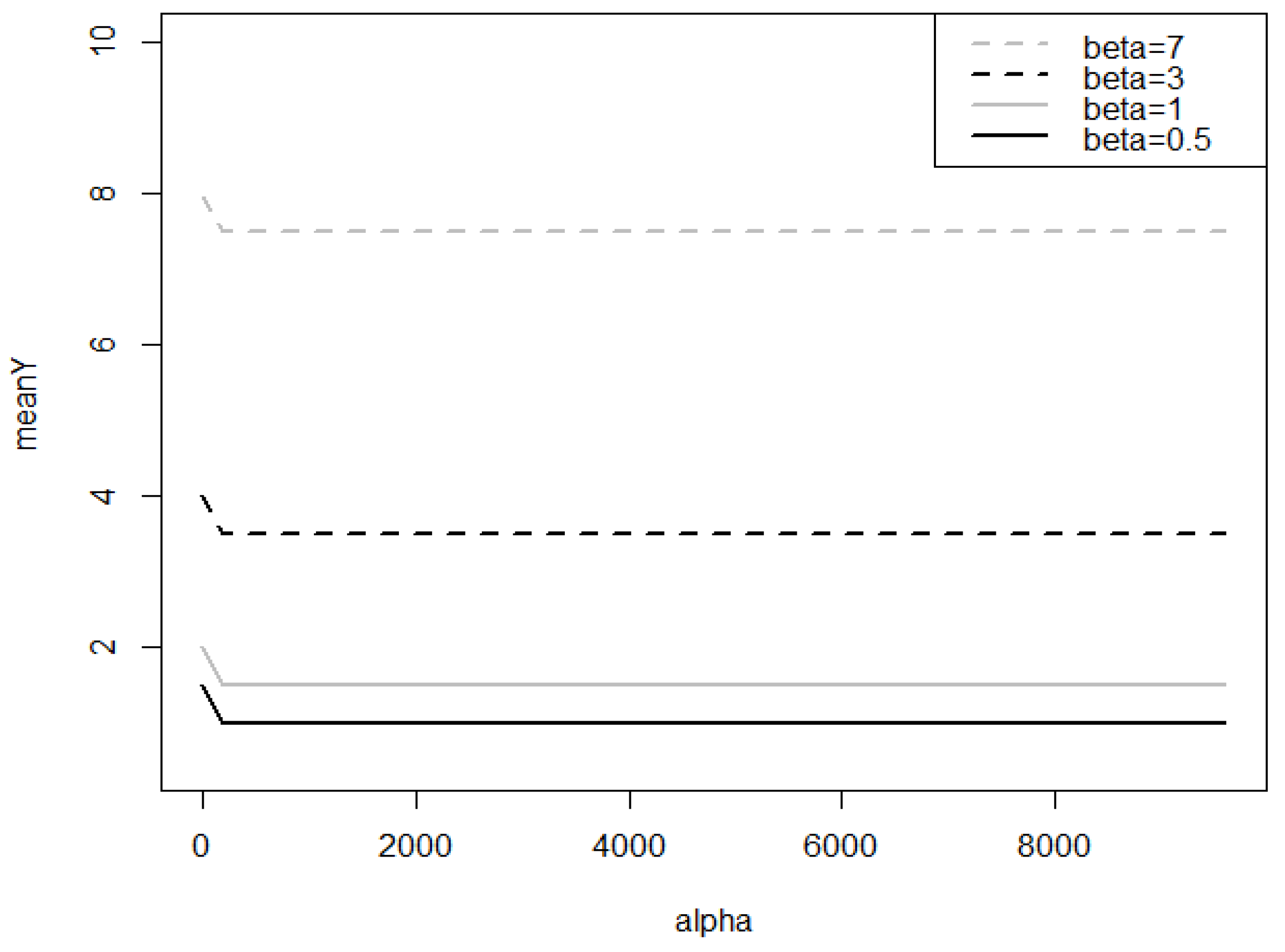
Figure 1. Computation of the mean of gamma-count distribution according to α and β = 0.5 , 1 , 3 , 7 .
Stats 06 00076 g001
Figure 2. Some gamma-count distributions according to (a) α = 1.2 and also to (b) β = 5 fixed.
Stats 06 00076 g002
Figure 3. Gamma-count (GC), double Poisson (DP) kernels with parametrization ( x + h , 1 / h ) compared to binomial (B) and CoM-Poisson (CMP) at x = 0 with (a) h = 0.01 ; (b) h = 0.1 ; (c) h = 0.3 .
Stats 06 00076 g003
Figure 4. Double Poisson and gamma-count kernels with parametrization ( x + h , 1 / h ) compared to CoM-Poisson (CMP) and binomial kernels at x = 5 with (a) h = 0.1 ; (b) h = 0.5 ; (c) h = 0.9 .
Stats 06 00076 g004
Figure 5. True pmf and estimate ones by gamma-count (GC), double Poisson (DP), binomial (B) and CoM-Poisson (CMP) kernels for the bimodal Scenario C with (a) n = 50 ; (b) n = 250 .
Stats 06 00076 g005
Figure 6. Empirical frequency with its corresponding gamma-count (GC), double Poisson (DP), binomial (B) and CoM-Poisson (CMP) kernel estimates of count dataset of insect pests on Hura trees with n = 51 .
Stats 06 00076 g006
Table 1. Comparison of execution times (in seconds) for one replication of Scenario C using gamma-count (gc), double Poisson (dp), binomial (b) and CoM-Poisson (cmp) kernel estimates.
n t gc t dp t b t cmp
200.147571.372900.0734351.82259
500.222564.638620.14665126.42510
1000.4229810.535220.16610263.30720
2500.7967317.081820.25914467.66510
5001.8256032.714560.49030945.52740
Table 2. Empirical mean values ( × 10 3 ) of I S E ^ n with their standard deviations in parentheses over N s i m = 500 replications and with different sample sizes n = 10 , 25 , 50 , 100 , 250 , 500 under four Scenarios A, B, C and D by using gamma-count (gc), double Poisson (dp), binomial (b) and CoM-Poisson (cmp) kernel estimators with the I S E bandwidth selection.
n ISE ^ gc , n ISE ^ dp , n ISE ^ b , n ISE ^ cmp , n
A109.2240 (7.9708)8.2596 (6.9910)24.5732 (19.0226)17.7012 (23.1386)
253.4346 (2.2426)4.0327 (2.5589)8.5250 (5.8778)9.3622 (11.2054)
502.9191 (2.0443)3.5842 (2.7603)4.5986 (3.0472)5.4105 (4.0815)
1001.8657 (1.2710)2.0070 (1.6637)2.2286 (1.3852)2.7595 (2.2578)
2500.9299 (0.7017)0.9670 (0.7401)1.2736 (0.8046)1.2511 (0.9823)
5000.5621 (0.3472)0.5906 (0.3923)1.2451 (0.6987)0.3669 (0.3047)
B109.9963 (8.2902)10.4663 (8.8282)25.3129 (13.1625)26.0588 (26.1514)
254.9811 (3.2787)5.4373 (4.2802)11.1561 (5.4033)10.5811 (8.4023)
503.1851 (2.2039)3.2929 (2.6541)5.0259 (3.1212)5.7034 (3.4369)
1002.2802 (1.2304)1.8941 (1.3242)2.8072 (1.4701)3.3802 (2.0909)
2501.7360 (0.7059)1.0332 (0.6626)1.3826 (0.6745)1.0374 (0.7745)
5001.5323 (0.5410)0.6010 (0.6010)0.8543 (0.3585)0.6245 (0.4315)
C1010.1931 (7.5874)11.2862 (7.3767)20.3614 (10.5060)23.3991 (20.7747)
255.3461 (3.8926)5.3975 (3.5143)8.1700 (4.1344)10.5258 (8.6422)
504.1610 (2.9936)4.0950 (2.6204)4.8990 (3.1218)5.0903 (4.2856)
1002.9958 (2.0992)2.1094 (1.7659)2.8961 (2.6908)3.0479 (2.1213)
2502.6143 (1.7647)1.5706 (1.2562)2.0777 (2.4729)0.8465 (0.5463)
5002.3825 (1.4641)1.0457 (1.1703)1.6664 (2.4254)0.4847 (0.2213)
D104.8289 (2.9155)4.9263 (2.9017)27.3001 (10.7675)10.7178 (20.0109)
252.3274 (1.5628)2.5004 (1.5756)9.4341 (3.6559)9.8068 (9.6282)
501.6284 (1.0325)1.8046 (1.2067)4.8759 (1.9313)2.1646 (1.8732)
1000.9935 (0.4916)1.0355 (0.6685)2.4179 (0.9076)1.1866 (0.7682)
2500.5522 (0.5522)0.5493 (0.3678)0.9362 (0.4277)0.4444 (0.3726)
5000.4297 (0.2286)0.3738 (0.2110)0.5068 (0.1881)0.3746 (0.2075)
Disclaimer/Publisher’s Note: The statements, opinions and data contained in all publications are solely those of the individual author(s) and contributor(s) and not of MDPI and/or the editor(s). MDPI and/or the editor(s) disclaim responsibility for any injury to people or property resulting from any ideas, methods, instructions or products referred to in the content.